Accuracy and Computational Efficiency of a Graphical Modeling Approach to Linkage Disequilibrium Estimation

Abstract

We develop recent work on using graphical models for linkage disequilibrium to provide efficient programs for model fitting, phasing, and imputation of missing data in large data sets. Two important features contribute to the computational efficiency: the separation of the model fitting and phasing-imputation processes into different programs, and holding in memory only the data within a moving window of loci during model fitting. Optimal parameter values were chosen by cross-validation to maximize the probability of correctly imputing masked genotypes. The best accuracy obtained is slightly below than that from the Beagle program of Browning and Browning, and our fitting program is slower. However, for large data sets, it uses less storage. For a reference set of n individuals genotyped at m markers, the time and storage required for fitting a graphical model are approximately O(nm) and O(n+m), respectively. To impute the phases and missing data on n individuals using an already fitted graphical model requires O(nm) time and O(m) storage. While the times for fitting and imputation are both O(nm), the imputation process is considerably faster; thus, once a model is estimated from a reference data set, the marginal cost of phasing and imputing further samples is very low.

1. Introduction

The increasing availability of genome-wide dense single-nucleotide polymorphism (SNP) data provides an abundance of information for gene mapping studies. However, along with the benefits provided by this new information come the difficulties posed by allelic associations. From a gross standpoint, the structure of allelic associations along a chromosome is largely dependent on distance, as a result of historical recombination events. However, on the fine scale of dense genotype assays, the patterns of association are highly complex, the result of the interplay between recombination, mutation, selection, and random drift (Chapman and Thompson, 2003). Failure to account for linkage disequilibrium (LD) may skew the results of linkage or association studies (Amos et al., 2006), thus providing a need for appropriate and efficient methods to model LD on a genome-wide level.

A variety of methods have been developed to address the problem of modeling LD. One class of such methods, including FastPHASE (Scheet and Stephens, 2006), Mach (Li et al., 2006) and Impute (Marchini et al., 2007), relies on the Li and Stephens (2003) model in which the haplotype in a neighborhood of each locus belongs to one of several haplotype clusters. Each individual’s cluster membership is allowed to change over the length of the chromosome, according to a Markov model. Browning and Browning (2008) take a different approach in their Beagle software, using variable length Markov chains (Browning, 2006) to model the dependence structure between alleles along the chromosome. While not always made explicit, all of the above approaches use special cases of graphical models (Lauritzen and Spiegelhalter, 1988) and depend on these structures for their computational efficiency. The model used by Browning and Browning, for instance, is a split graphical model. Thomas and Camp (2004) were the first to estimate general decomposable graphical models for the joint distribution of allele frequencies. They estimated the models from phased haplotypes by incorporating Markov chain Monte Carlo (MCMC) into the method of (Høsgaard and Theisson, 1995). Thomas (2005) then extended the method to the case of genotype data using an iterative approach.

One critical consideration in the use of MCMC to estimate graphical models for LD is that computations on graphical models are tractable only for the case of decomposable, or triangulated, graphs (Lauritzen and Sheehan, 2003). This poses a problem in the straightforward use of a general graphical model for LD, since the connection or disconnection of randomly-selected vertices does not, in general, preserve decomposability. In fact, the proportion of decomposable graphs proposed tends to decrease inversely with the number of loci (Thomas and Green, 2009a), resulting in a highly inefficient sampler. In order to circumvent this problem, Thomas (2009a,b) restricted the class of graphical models to the set of interval graphs, in which the vertices of the graph are represented by intervals of the real line and are connected exactly when the intervals intersect. The resultant sampler was efficient and mixed well. Furthermore, the restriction to interval graphs facilitated a windowing scheme which allowed the program’s time and memory requirements to increase linearly in the number of loci, making genome-wide analyses feasible.

The current work uses an MCMC method for estimating LD using a more general, and hence more flexible, class of decomposable graphical models. Our new model allows for a general decomposable graph representation of the allele frequency dependence structure, with the restriction that loci too distant from one another must be conditionally independent. This simplification reflects biological expectations and again permits a windowed approach, allowing for a linear increase in runtime with number of loci. Furthermore, our sampler benefits from a method, recently described by Thomas and Green (2009a,b), to sample only the space of decomposable graphs. This sampler traverses the space of decomposable models more efficiently than the straightforward rejection method of Giudici and Green (1999), for example.

In this study we show that our more general class of graphical models is more accurate than interval graph models and gives imputation accuracy comparable to that had by the Beagle program. Moreover, we show that our approach has computational complexity that is linear in the number of loci and only slightly super linear in the number of individuals, which, along with our efficient use of memory, allows our program to perform genome-wide analyses on thousands of individuals.

2. Methods

2.1. Model estimation

Graphical modeling is a useful approach to modeling the joint distribution of a set of dependent random variables {X₁, X_s, …X_n} when many of the variables are independent conditional on other variables. That is, when the joint distribution can be factored as $f(X_1,X_2,\dots X_n)={\prod }_{i=1}^{k}f(T_i)$, when the T_i are small subsets of {X₁, X_s, …X_n}. To this factorization corresponds a Markov, or conditional independence, graph, which has the variables as vertices and in which an edge connects any two vertices contained in the same set T_i.

In the case of LD, we expect the joint distribution of allele frequencies to exhibit such a factorization since historical recombination tends to result to conditional independence between distant loci. Given phased haplotype data for n loci, a graphical model for the joint distribution of alleles can be estimated as in Thomas and Camp (2004) according to the method of Høsgaard and Theisson (1995). Briefly, the sampled haplotypes are regarded as drawn from a multinomial distribution P(X₁, X₂, …, X_n) in which the conditional independence structure between the alleles {X_i} is described by a decomposable graphical model G, that is, a graphical model with decomposable, or triangulated, Markov graph. The graphical model G is estimated as follows. Given an incumbent decomposable graph G describing the allelic associations, G is perturbed to give a new graph G′. If G′ is decomposable, it has the running intersection property. That is, its maximal complete subgraphs, or cliques, C₁,C₂,...C_k, can be ordered such that

$$S_i\equiv C_i\cap {\cup }_{j>i}{C}_j\subset C_l,$$

for some l > i. Thus its joint probability distribution factors as

$$P(X_1,X_2,\dots ,X_n)=\prod _{i=1}^{k}P(C_i|S_i)=\prod _{i=1}^k\frac{P(C_i)}{P(S_i)}.$$

Intuitively, the necessity of the running intersection property is that it imposes an order on the cliques that permits the use of standard forward-backward algorithms (Baum et al., 1970) for sampling and maximization.

Since the distributions for the C_i and S_i are described by contingency tables, whose degrees of freedom and maximized likelihoods are straightforward to calculate, the maximized log-likelihood and degrees of freedom for a model with Markov graph G can be computed as:

$$df(G)=\sum _{i=1}^{k}df(C_i)-\sum _{i=1}^{k}df(S_i)\hspace{0.17em}\hspace{0.17em}\hspace{0.17em}\hspace{0.17em}\hspace{0.17em}\hspace{0.17em}\hspace{0.17em}\text{and}$$ (1)

$$\text{log}\widehat{L}(G)\equiv \underset{M}{\text{max}}\hspace{0.17em}\text{log}L(G,M)=\sum _{i=1}^k\text{log}\widehat{L}(C_i)-\sum _{i=1}^k\text{log}\widehat{L}(S_i)$$ (2)

for M, the set of multinomial parameters. Thomas and Camp (2004) used simulated annealing to sample the space of decomposable graphs. With probability

$$\text{max}\{1,{(\frac{e^{IC(G^{\prime })}}{e^{IC(G)}})}^{1/t}\},$$ (3)

G′ becomes the new incumbent graph. Otherwise the graph G remains. Here t is the temperature parameter for the simulated annealing and

$$IC(G)=\mathit{\text{log}}\widehat{L}(G)-\alpha df(G)$$ (4)

is a penalized log-likelihood.

The extension to unphased genotype data is carried out iteratively as detailed in Thomas (2005). Given a graphical model G for the LD, G is applied to both the maternal and paternal haplotypes of each individual. Let Y_ij, M_ij, F_ij, and E_ij be the observed genotype data, maternal allele, paternal allele, and error indicator, respectively, for individual i at locus j, with M⃗_i and F⃗_i his paternal and maternal haplotypes. Then the model likelihood is

$$P(Y|G)=\sum _E\sum _M\sum _F\prod _{i}P({\overrightarrow{M}}_i|G)P({\overrightarrow{F}}_i|G)\prod _{j}P(Y_{ij}|M_{ij},F_{ij},E_{ij})P(E_{ij}),$$

for generalized penetrance function P(Y_ij|M_ij, F_ij, E_ij) (Thomas, 2005). Note that, in this case, with the Y_ij as genotype data, the generalized penetrance serves to account for genotyping error. However, in the straightforward extension of the Y_ij to include, for instance, disease phenotypes or covariates, the generalized penetrance allows for disease penetrance as well as observational error. For each individual i, M⃗_i, F⃗_i, and E⃗_i can be sampled in a single blocked Gibbs update (Dawid, 1992; Jensen and Kong, 1996), with probability proportional to

$$P({\overrightarrow{M}}_i|G)P({\overrightarrow{F}}_i|G)\prod _{j}P(Y_{ij}|M_{ij},F_{ij},E_{ij})P(E_{ij}).$$ (5)

2.2. Computational efficiency

Consider the problem of estimating a graphical model from a set of m loci genotyped on a reference set of n individuals. In our approach we restrict the general class of decomposable graphical models for LD to those with conditional independence graphs connecting loci separated by at most v intervening SNPs. This simplification keeps with biological expectations and so is unlikely to adversely affect the LD model estimate. By allowing for a windowing approach, it does, however, render the implementation much more computationally tractable.

In estimating a graphical model from genotype data, two moving windows are used, each containing w consecutive loci. The first window moves along the chromosome by jumps of one-half the window width; the second window proceeds similarly, but lags a half window width behind the first. In the first window, random sampling is carried out: an average of p Metropolis updates per locus are performed by sampling the space of junction trees, each update proposing a decomposability-preserving connection or disconnection of a pair of vertices (Thomas and Green, 2009a,b), with acceptances determined according to the penalized likelihood (4) and the Metropolis acceptance rule, that is, according to (3) with t = 1. Every g Metropolis updates of the graph, a blocked Gibbs method is used to update the phases according to the current estimate of the graphical model. The second window performs the uphill search. In this window, a new graph proposal is accepted only if it has penalized likelihood at least as large as the incumbent, that is, according to (3) with t = 0; updated phases are determined by the most probable phase, rather than as a random Gibbs sample. The windows move together along the genome so that the model space is searched in a single pass. Only the data required for the current windows is held in memory at any time, so that the maximum storage requirement for the genetic data is of order O(n). As the graphical model is built, it is stored and output at the end of the program, requiring storage of O(m). The total storage required is thus O(n + m).

The number of Metropolis updates made to the model in any window is wp, and the Gibbs updates of phase require time proportional to the number of variables involved. Since these are made for each individual but only for loci within windows, this time requirement is proportional to wn. The windows shift by half a window length after each set of updates, hence the total time required is O(nm).

This model estimation approach requires us to hold data for all individuals simultaneously but for only a small number of loci. In contrast, in order to impute phases and missing data by the usual forward-backward graphical model algorithm, we need to hold data for only one individual at a time, but for all loci. For this reason, we separate the model fitting and imputation problems into different programs. The graphical model estimated by the first program is input into the second and applied to the data for each individual in turn. The total storage requirement for imputation is thus O(m). The time required is O(nm), but note that the implied constant here is far smaller than that for the O(nm) in model estimation. In order to mimic the analysis of, for instance, Beagle, the same input data is used for both the fitting and imputation programs; however, note that this need not be the case. The model obtained by the fitting method can be applied to any individuals genotyped at the same loci. Hence, although estimating a model on a large data set can be computationally expensive, this overhead is mitigated by the low marginal cost of imputing further samples.

2.3. Implementation

The above methods are implemented as parts of a set of Java Programs for Statistical Genetics and Computational Statistics (JPSGCS) distributed by Alun Thomas (http://balance.med.utah.edu/wiki/index.php/JPSGCS). As with other programs in the package, the data file formats defined by the LINKAGE program (Lathrop and Lalouel, 1984) are used; however, some modifications are required. Specifically, since the LINKAGE genotype data file lists the genotypes for each individual line by line, it is suitable for use by our imputation program. It is however in the wrong orientation for the estimation program, so we provide a utility to transpose it. Also, the LINKAGE parameter file has no support for complex LD models, thus we append our graphical model to a standard LINKAGE parameter file. The three programs we provide are TransposeLinkage to modify the LINKAGE genotype file, FitGMLD to fit the graphical model, and Complete to impute phase and missing data.

Suppose that we have data specified in the usual LINKAGE format in two files: input.par containing information about the genetic loci, and input.ped containing the genotypes. Note that input.ped is also used to specify relationships between individuals, but that any such relationships are ignored by these programs which assume that our data come from a random population sample. The following sequence of commands would run the estimation and imputation processes. Here, p and g are the numbers of Metropolis and Gibbs updates per window, respectively; w is the window width; v, the maximum number of loci intervening between two connected loci; and q determines the complexity penalty α in (4) by α = 0.5 * qlog 2n.

% java TransposeLinkage input.par input.ped > transpose.ped

% java FitGMLD input.par transpose.ped v w g p q > output.ld.par

% java Complete output.ld.par input.ped > output.ped

The final phased data is given in output.ped. Like the original input file, this is a LINKAGE format pedigree file, but it will have no missing genotypes, and the order in which alleles are listed specifies the imputed phase.

The file output.ld.par contains the data in input.par but with the LD model appended. As well as being input to the Complete program, this can be used for other purposes, for instance, the previously described GeneDrop program (Thomas et al., 2008) will simulate data in a pedigree using the LD model to generate founder haplotypes and the usual gene drop approach (MacCluer et al., 1986). For example, to simulate data for the pedigree described in the file simin.ped and put the output into a file called simout.ped we can use:

% java GeneDrop output.ld.par simin.ped > simout.ped

2.4. Parameter optimization

We determined optimal settings for the parameters v, w, and q by cross-validation on contiguous subsets of SNPs from HapMap data. We used the data on chromosome 1 for 60 unrelated individuals for the Yoruba people of Ibadan, Nigeria (The International HapMap Consortium, 2007). For each set of parameter values, we scored the accuracy by masking at random 15% of the genotypes and then determining the percentage correctly imputed. Convergence was assessed by a stable, with respect to number of MCMC iterations, penalized model log-likelihood. For the purposes of parameter optimization, we fixed p = 1000 and g = 20. This was a conservative choice for most parameter combinations tested. Increasing v and decreasing q both increase the model search space, however, so that p =1000, g = 20 was not adequate to ensure convergence in the extremes of these settings. Effectively, we have added a constraint to the optimization problem, such that we now seek optimal parameter settings for a sampler that must converge within a reasonable number of iterations, hence runtime.

The main purpose of the window width parameter w is to ensure that the run time and memory usage of the program scales linearly in the number of loci (Thomas, 2009b). As long as the window width was not too short (less than approximately 200 loci), variation in this parameter had little effect on the imputation accuracy of FitGMLD across a range of penalty multipliers (q between 0.0625 and 2.0) and maximum link distances (v between 5 and 55). Since the computational burden increases with window width, we took w = 250 as the default window width.

The maximum link distance v and the penalty multiplier q both serve to limit the model complexity, but in somewhat different ways. Restricting v disallows edges between loci that are too far linearly separated along the chromosome, whereas increasing q reduces model complexity by disregarding the overall least significant allelic associations. Finally, we compared the accuracy and runtime for FitGMLD to those of Beagle under its default settings. All results were obtained on a 2.5 GB partition of 2.93 GHz Intel Xeon processor with 14GB RAM.

3. Results

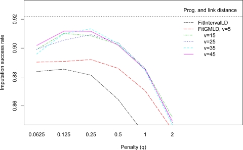
FitGMLD and Complete performed well, achieving over 90% imputation accuracy, for a range of reasonable parameter combinations. Figure 1 depicts the effects of varying v and q on the success rate of FitGMLD and a comparable interval graph method, FitIntervalLD, for missing data imputation. Across all combinations of w, q, and v tested, FitGMLD outperformed FitIntervalLD. FitGMLD (maxlink v = 5), performed best with less additional constraint (lower penalty), illustrating the tradeoff between penalty and maxlink. However, these more restrictive models gave less accurate results, due to their oversimplification of allelic associations. For runs of FitGMLD with maxlink at least 15, optimal imputation success was attained with penalty, q, between 0.125 and 0.25. Since the computational burden increases with decreasing penalty and increasing maximum link distance, we use q = 0.25 and v = 15.

Figure 1:

Success rate for missing data imputation for FitGMLD, by penalty and maximum link distance (window width=250), compared to FitIntervalLD. The horizontal dotted line represents Beagle’s imputation success.

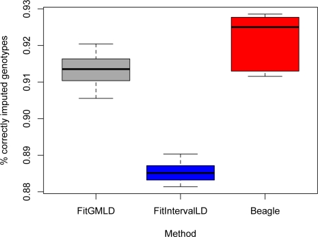
With properly tuned parameters, FitGMLD consistently outperformed Fit-IntervalLD but was slightly less accurate than the Beagle (Beagle version 3.0.4) software (Browning and Browning, 2008). In accordance with Figure 1, we took as optimal parameters (w, v, q) = (250, 15, 0.25) for FitGMLD and penalty q = 0.125 for FitIntervalLD. Figure 2 shows the fraction of genotypes correctly imputed of the 15% that were randomly deleted, for a set of 500 contiguous SNPs (5 independent estimates). Of the three programs, Beagle achieves the best mean accuracy (92.1%), and FitGMLD (91.3%) performs almost as well. The accuracy of FitIntervalLD (88.5%) is lower, which is expected since it models LD by a more restrictive class of graphs. These results were independent of the experimental design. For example, we observed similar performance imputing genotypes for a test set genotyped at a sparse subset of loci, given a fully genotyped reference set. The accuracies do, as expected, tend to increase with the number of loci, reaching, for 100,000 loci, approximately 93% and 95% with FitGMLD and Beagle, respectively.

Figure 2:

Success rate for missing data imputation, comparison of FitGMLD, Fit-IntervalLD, and Beagle for 500 loci, 5 independent estimates each.

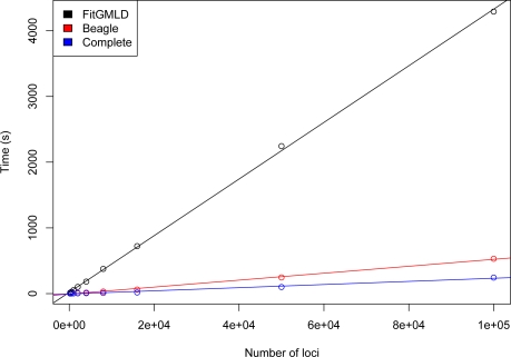
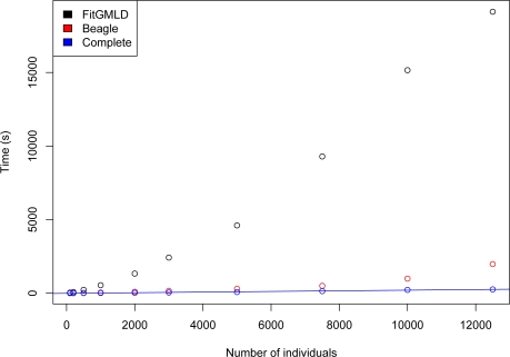
Use of a full graphical modeling approach to estimate LD is computationally intensive, as reflected in the relatively long runtimes of FitGMLD. Figure 3 compares the run times of FitGMLD, Beagle, and Complete on contiguous subsets of of 200 to 100,000 loci on chromosome 1 from 60 unrelated individuals from the HapMap Yoruba data set. As shown, all three programs scale approximately linearly in the number of loci. Figure 4 compares the run times of FitGMLD, Beagle, and Complete on data for 500 loci from sets of 100 to 12500 individuals. These data were simulated according to a previously estimated LD model. Complete scales linearly in the number of sampled individuals, whereas the runtimes for FitGMLD and Beagle both exhibit slight super-linear growth in the number of samples. In the case of FitGMLD, the super-linearity reflects increased estimated model complexity with increasing sample size.

Figure 3:

Time to run FitGMLD (black), Beagle (red), and Complete (blue) vs. number of markers, for 60 individuals.

Figure 4:

Time to run FitGMLD (black), Beagle (red), and Complete (blue) vs. number of individuals, for 500 loci.

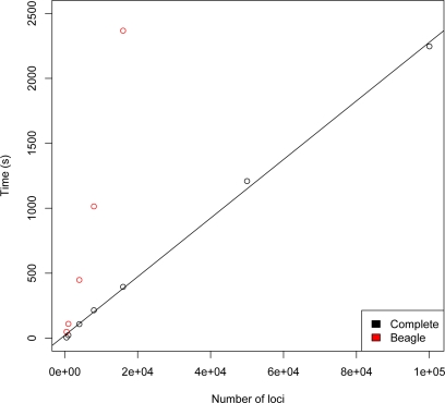
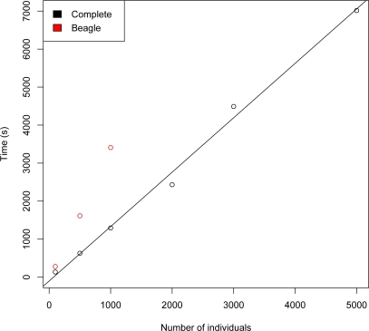
The graphical modeling approach requires a relatively long time to estimate a joint allelic distribution. Once estimated, however, a reference LD model can be used for a variety of purposes, including imputing missing data from additional test sets. In this case, imputation is quite fast. Figure 5 shows the time to phase 1000 simulated genotypes for 200 to 100,000 loci for both Complete and Beagle. Figure 6 shows the time to phase simulated genotypes with 50,000 markers for 100 to 5000 individuals for Complete and Beagle. Again, Complete is fast and scales linearly in the number of individuals.

Figure 5:

Time to run Complete (black) or Beagle (red) vs. number of markers for 1000 individuals.

Figure 6:

Time to run Complete (black) and Beagle (red) vs. number of individuals for 50,000 markers.

4. Conclusions

We have shown that it is feasible to model allelic associations by a fairly general class of decomposable graphs. As illustrated by comparison with the Beagle software package, our algorithm attains accuracy in imputing missing genotypes comparable to that of other current programs. Our model, however, allows for both genotyping error and complex patterns of linkage disequilibrium that are only loosely bound to the physical order to loci along a chromosome. Thus the model estimation step of our approach is much slower than Beagle’s simple and efficient strategy of estimating variable length Markov chains by first constructing a tree of all possible haplotypes and then merging nodes whose state is independent of the states of downstream loci. In some cases, our approach may better model the fine structure of allelic associations, which is shaped less by recombination than by new mutations arising on different genetic backgrounds. Furthermore, while the imputation accuracy of our method was slightly less than that of Beagle for the particular test data chosen here, its greater flexibility might prove important for genetic data containing many cryptic rearrangements.

The generality of our graphical modeling approach to estimating allelic associations comes at a cost; the programs are computationally expensive. Compared to other schemes for estimating LD, however, our method does enjoy several advantages. First, our two-stage LD model estimation and haplotype phasing is efficient in its use of memory. Our implementation allows for model estimation from an arbitrarily large reference panel. Furthermore, after a reference LD model has been estimated, the Complete program can quickly phase haplotypes and impute missing data for arbitrarily large sample sizes.

Our use of a Markov chain Monte Carlo approach permits, in addition to posterior most probable imputation, simulation from the posterior distribution on all variables, so that we can assess confidence in our imputations. Marginal posterior distributions for locus genotypes can also be computed to give confidence indicators. Also, genotyping error is explicitly included in both our model estimation and imputation programs. This not only renders our estimates robust to genotyping error but also allows for estimating the posterior probabilities of such errors.

An important advantage of our approach is that the output of our model estimation program is a well-defined joint posterior probability distribution on the marker states. This provides several benefits. Once an LD model has been estimated for a suitable reference set, such as from the HapMap or 1000 Genomes projects, subsequent haplotype phasing or imputation of missing data in test sets can be performed very quickly. The haplotype frequency model can also be used to control for allelic associations in a variety of other analyses. For example, the LD model can be incorporated into simulation methods used to generate empirical p-values in, for instance, methods to detect identity by descent from dense SNP data (Thomas, 2007; Thomas et al., 2008). They can also be used for imputation across SNP genotyping platforms, similar to the BeagleCall software (Browning and Yu, 2009). A final advantage of our general graphical modeling approach is its straightforward extension to include discrete covariates, such as an individual’s population of origin, and outcome variables, facilitating, for instance, the detection of phenotype-haplotype associations, while controlling for population stratification.

References

- Amos C, Chen W, Lee A, Li W, Kern M, Lundsten R, Batliwalla F, Wener M, Remmers E, Kastner D, Criswell L, Seldin M, Gregersen P. “High-density SNP analysis of 642 Caucasian families with rheumatoid arthritis identifies two new linkage regions on 11p12 and 2q33.”. Genes Immun. 2006;7:277–86. doi: 10.1038/sj.gene.6364295. [DOI] [PubMed] [Google Scholar]
- Baum LE, Petrie T, Soules G, Weiss N. “A maximization technique occurring in the statistical analysis of probabilistic functions of Markov chains,”. Annals of Mathematical Statistics. 1970;4:1, 164–171. [Google Scholar]
- Browning BL, Yu Z. “Simultaneous genotype calling and haplotype phasing improves genotype accuracy and reduces false-positive associations for genome-wide association studies,”. American Journal of Human Genetics. 2009;8:5, 847–861. doi: 10.1016/j.ajhg.2009.11.004. [DOI] [PMC free article] [PubMed] [Google Scholar]
- Browning SR. “Multilocus association mapping using variable-length markov chains”. American Journal of Human Genetics. 2006;78:903–913. doi: 10.1086/503876. [DOI] [PMC free article] [PubMed] [Google Scholar]
- Browning SR, Browning BL. “Rapid and accurate haplotype phasing and missing data inference for whole genome association studies by use of localized haplotype clustering”. American Journal of Human Genetics. 2008;81:1084–1097. doi: 10.1086/521987. [DOI] [PMC free article] [PubMed] [Google Scholar]
- Chapman N, Thompson E. “The effect of population history on the lengths of ancestal chromosome segments,”. Genetics. 2003;6:4, 449–458. doi: 10.1093/genetics/162.1.449. [DOI] [PMC free article] [PubMed] [Google Scholar]
- Dawid A. “Applications of a general propagation algorithm for probabilistic expert systems,”. Statistical Computing. 1992;2:25–36. doi: 10.1007/BF01890546. [DOI] [Google Scholar]
- Giudici P, Green PJ. “Decomposable graphical Gaussian model determination,”. Biometrika. 1999;8:6, 785–801. [Google Scholar]
- Høsgaard S, Theisson B. “BIFROST–Block recursive models induced from relevant knowledge, observations, and statistical techniques,”. Computational Statistics and Data Analysis. 1995;1:9, 155–175. [Google Scholar]
- Jensen C, Kong A. “Blocking Gibbs sampling for linkage analysis in large pedigrees with many loops,”. 1996. Technical report, Department of Computer Science, Aalborg University. [DOI] [PMC free article] [PubMed]
- Lathrop GM, Lalouel J. “Easy calculations of lod scores and genetic risks on small computers,”. American Journal of Human Genetics. 1984;3:6, 460–465. [PMC free article] [PubMed] [Google Scholar]
- Lauritzen S, Sheehan N. “Graphical models for genetic analyses,”. Statistical Science. 2003;1:8, 489–514. [Google Scholar]
- Lauritzen S, Spiegelhalter D. “Local computations with probabilities on graphical structures and their applications to expert systerms,”. Journal of the Royal Statistical Society Series B. 1988;50:157–224. [Google Scholar]
- Li N, Stephens M. “Modeling linkage disequilibrium and identifying recombination hotspots using single-nucleotide polymorphism data,”. Genetics. 2003;165:2213–2233. doi: 10.1093/genetics/165.4.2213. [DOI] [PMC free article] [PubMed] [Google Scholar]
- Li Y, Ding J, Abecasis G. “Mach 1.0: Rapid haplotype recontruction and missing genetype inference,”. American Journal of Human Genetics. 2006;79:S2290. [Google Scholar]
- MacCluer J, Vandeburg J, Read B, Ryder O. “Pedigree analysis by computer simulation,”. Zoo biology. 1986;5:147–160. doi: 10.1002/zoo.1430050209. [DOI] [Google Scholar]
- Marchini J, Howie B, Myers S, McVean G, Donnelly P. “A new multipoint method for genome-wide association studies via imputation of genotypes,”. Nature Genetics. 2007;3:9, 906–913. doi: 10.1038/ng2088. [DOI] [PubMed] [Google Scholar]
- Scheet P, Stephens M. “A fast and flexible statistical model for large-scale population genotype data: applications to inferring missing genotypes and haplotypic phase,”. American Journal of Human Genetics. 2006;7:8, 629–644. doi: 10.1086/502802. [DOI] [PMC free article] [PubMed] [Google Scholar]
- The International HapMap Consortium “A second generation human haplotype map of over 3.1 million SNPs,”. Nature. 2007;44:9, 851–861. doi: 10.1038/nature06258. [DOI] [PMC free article] [PubMed] [Google Scholar]
- Thomas A. “Characterizing allelic associations from unphased diploid data by graphical modeling,”. Genetic Epidemiology. 2005;2:9, 23–35. doi: 10.1002/gepi.20076. [DOI] [PubMed] [Google Scholar]
- Thomas A. “Towards linkage analysis with markers in linkage disequilibrium,”. Human Heredity. 2007;6:4, 16–26. doi: 10.1159/000101419. [DOI] [PubMed] [Google Scholar]
- Thomas A. “Estimation of graphical models whose conditional independence graphs are interval graphs and its application to modeling linkage disequilibrium,”. Computational Statistics and Data Analysis. 2009a;5:3, 1818–1828. doi: 10.1016/j.csda.2008.02.003. [DOI] [PMC free article] [PubMed] [Google Scholar]
- Thomas A. “A method and program for estimating graphical models for linkage disequilibrium that scale linearly with the number of loci, and their application to gene drop simulation,”. Bioinformatics. 2009b;2:5, 1287–1292. doi: 10.1093/bioinformatics/btp146. [DOI] [PMC free article] [PubMed] [Google Scholar]
- Thomas A, Camp NJ. “Graphical modeling of the joint distribution of alleles at associated loci,”. American Journal of Human Genetics. 2004;74:1088–1101. doi: 10.1086/421249. [DOI] [PMC free article] [PubMed] [Google Scholar]
- Thomas A, Camp NJ, Farnham J, Allen-Brady K, Cannon-Albright L. “Shared genomic segment analysis. mapping disease predisposition genes in extended pedigrees using SNP genotype assays,”. Annals of Human Genetics. 2008;72:279–287. doi: 10.1111/j.1469-1809.2007.00406.x. [DOI] [PMC free article] [PubMed] [Google Scholar]
- Thomas A, Green PJ. “Enumerating the decomposable neighbors of a decomposable graph under a simple perturbation scheme,”. Computational Statistics and Data Analysis. 2009a;5:3, 1232–1238. doi: 10.1016/j.csda.2008.10.029. [DOI] [PMC free article] [PubMed] [Google Scholar]
- Thomas A, Green PJ. “Enumerating the junction trees of a decomposable graph,”. Journal of Computational and Graphical Statistics. 2009b;1:8, 930–940. doi: 10.1198/jcgs.2009.07129. [DOI] [PMC free article] [PubMed] [Google Scholar]