A Statistical Approach for Breast Density Segmentation

Abstract

Studies reported in the literature indicate that the increase in the breast density is one of the strongest indicators of developing breast cancer. In this paper, we present an approach to automatically evaluate the density of a breast by segmenting its internal parenchyma in either fatty or dense class. Our approach is based on a statistical analysis of each pixel neighbourhood for modelling both tissue types. Therefore, we provide connected density clusters taking the spatial information of the breast into account. With the aim of showing the robustness of our approach, the experiments are performed using two different databases: the well-known Mammographic Image Analysis Society digitised database and a new full-field digital database of mammograms from which we have annotations provided by radiologists. Quantitative and qualitative results show that our approach is able to correctly detect dense breasts, segmenting the tissue type accordingly.

Introduction

Breast cancer is a major health problem in Western countries. A study developed by the American Cancer Society estimates that, in the USA, between one in 8 and one in 12 women will develop breast cancer during their lifetime.¹ In addition, a recent study of the Australian Institute of Health and Welfare shows that, in Australia, one in 36 woman deaths before the age of 85 are due to this disease.²

Mammography is still the most commonly used method for detecting breast cancer at early stages, a crucial issue for a high survival rate. With the name of computer-aided tools, there have recently appeared a set of computerised tools to assist physicians to detect and diagnose breast cancer.^3,4 However, recent studies have shown that the performance of these systems decreases as the density of the breast increases, either decreasing the sensitivity^5,6 or increasing the specificity.⁷ This is a real drawback, since it is widely known by the medical community that breast cancer risk increases as the breast density increases.⁸ Therefore, the segmentation of the breast density might be beneficial not only for estimating the quantity of breast dense tissue but also for establishing independent strategies in fatty or dense regions where an automatic procedure may be used to look for abnormalities.⁹

During the last years, different algorithms have been proposed for breast density segmentation. For instance, Boyd et al.¹⁰ and Sivaramakrishna et al.¹¹ used a grey-level thresholding technique to segment the breast into dense and fatty regions. In contrast of obtaining just two clusters, Ferrari et al.¹² and Aylward et al.¹³ used mixtures of Gaussian for modelling and segmenting the breast into four and five regions, respectively. However, these related approaches do not take spatial information into account, providing segmentations with too many disconnected regions. Moreover, an initial pre-processing step is needed to remove noisy pixels. Aiming to include this spatial information into account, Saha et al.¹⁴ included a fuzzy affinity function in their proposal, while Zwiggelaar and Denton¹⁵ and Petroudi and Brady¹⁶ employed textural features to take the spatial distribution of the pixel and its neighbourhood into account.

In this paper, we present a statistical approach, which also uses spatial information, to perform breast parenchyma segmentation. The approach is based on modelling a set of patches of either fatty or dense parenchyma using statistical analysis. In particular, we analyse two different strategies to perform this modelling process: (1) Karhunen–Loeve-based model [principal component analysis (PCA)] and (2) linear-discriminant-based model [linear discriminant analysis (LDA)]. Once the tissue models have been learned, each pixel of a new mammogram is classified as being fatty or dense tissue, taking its corresponding neighbourhood into account. Note that we perform pixel-based segmentation but using spatial information from the neighbourhood model in the classification step. The final result of our approach is a segmented mammogram with two different regions according to the breast tissue. In order to evaluate our segmentation proposal, we present quantitative and qualitative results extracted from two different databases: the well-known Mammographic Image Analysis Society (MIAS) database and a new full-field digital database of mammograms from which we have expert annotations.

The rest of the paper is structured as follows. The next section describes the used databases as well as the segmentation approach. Experimental results are then presented in “Results”. The analysis of these results as well as a comparison with other approaches is presented in “Discussions”. Finally, the paper ends with “Conclusions”.

Materials and Methods

In this section, we describe the proposed approach for breast density segmentation. However, we first present the databases used in the experimental section.

Databases

We test our approach using two different databases: the MIAS database and the Trueta database.

The MIAS Database

The MIAS database¹⁷ contains mammograms extracted from the UK National Breast Screening Programme and digitised to 50- × 50-μm pixel resolution with a Joyce–Loebl scanner. The database includes MLO views of both left and right breasts, expert annotations [including presence and location of abnormalities (if any)] and a breast density classification with three categories: fatty, glandular and dense (in density increasing order). However, and due to the increasing usage of the breast imaging reporting and data system (BIRADS) standard, we asked three expert radiologists to classify the set of mammograms according to the BIRADS standard (a majority vote between the three experts was used to provide the used BIRADS density classification). Table 1 shows the distribution of this expert classification. As it is shown in the table, a strong correlation exists between fatty breasts and low BIRADS classes and also between dense breasts and high BIRADS classes.

Table 1.

Confusion Matrix Between the Classification of MIAS Mammograms According to its Annotations (Fatty, Glandular and Dense) or the Consensus of Three Radiologists in BIRADS Terms

	B-I	B-II	B-III	B-IV	Total
Fatty	83	23	0	0	106
Glandular	4	60	38	2	104
Dense	0	20	57	35	112
Total	87	103	95	37	322

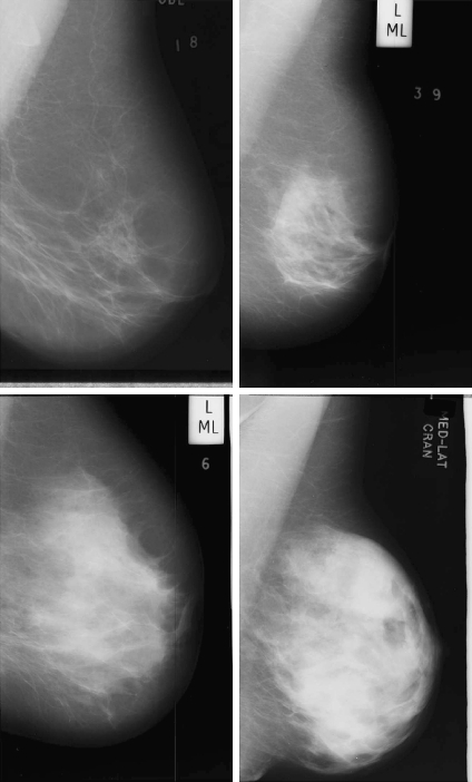
Figure 1 shows four mammogram examples of this database with increasing internal density (from BIRADS I to BIRADS IV). In general, the brighter the pixel, the denser the tissue is. Note that the pectoral muscle appears in the top-right corner of the images, and there are also some annotations outside the breast area. Hence, the initial step of our proposal should be able to separate the breast region from the other ones.

Fig 1.

Four mammogram examples from the MIAS database with increasing density (from left to right and top to bottom).

The Trueta Database

The second database used is the Trueta Database. The mammograms of this database are obtained by a full-field digital Siemens Mammomat Novation mammograph, and the images are stored according to the DICOM protocol. There are two different image sizes depending on the breast size: 2,560 × 3,328 or 3,328 × 4,096 pixels, being the resolution of each image 70- × 70-μm pixel. In this work, we use a subset containing 125 CC and 125 MLO views of the same breast of 75 women (there are 50 complete cases—MLO and CC views of left and right mammograms of the same patient—and 25 where the MLO and CC of only one breast is available). Regarding the annotations, two radiologists classified the entire database according to the BIRADS standard, obtaining 96 BIRADS I, 40 BIRADS II, 74 BIRADS III and 40 BIRADS IV mammograms. In addition, the radiologists provided detailed dense regions annotations (ground-truth segmentation) for 60 mammographic images, accurately surrounding the region using a digital pen. In particular, the radiologists annotated 15 MLO images randomly selected from the database of each BIRADS class.

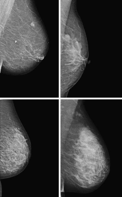
Figure 2 shows four mammograms of this database with increasing internal density (from BIRADS I to BIRADS IV). Note that the pectoral muscle still appears in the top-right image corners, while the text annotations are now removed.

Fig 2.

Four mammograms examples from the Trueta database with increasing density (from left to right and top to bottom).

Initial Pre-processing Step

As already explained, the first step of our approach consists in segmenting the background, annotations and the pectoral muscle of the images. Note that background subtraction is needed to correctly focus the algorithm. Moreover, we need to extract the pectoral muscle because, in some mammograms, it has a similar appearance than the dense tissue, leading to incorrect segmentations. This can be clearly seen in the last image of Figure 1.

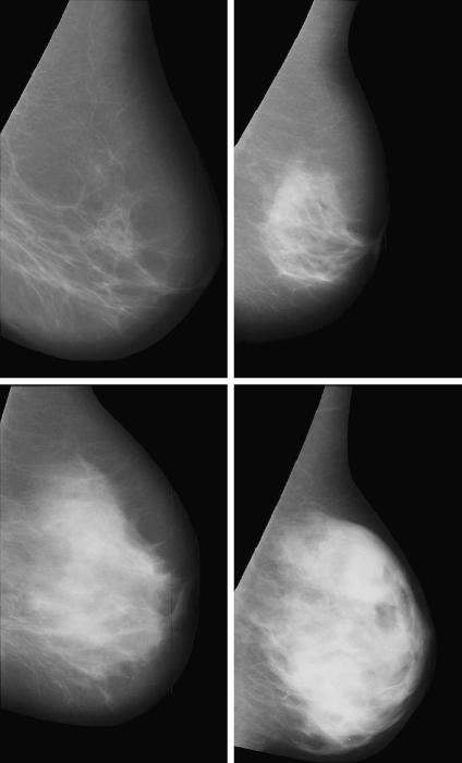
We used the approach developed by Martí et al.¹⁸ to identify the region composed by the breast and the pectoral muscle. Briefly, the method starts by computing a scale space representation of the image in order to perform edge detection using different scales. Subsequently, an initial seed point lying in the skin-line contour is automatically located, and it is used as the starting point of a contour growing process, which is guided by attraction and regularisation forces. Afterwards, we use the proposal of Kwok et al.¹⁹ to detect and remove the pectoral muscle. In this approach, the pectoral edge is firstly estimated by a straight line that is validated for correctness of location and orientation. This estimate is then refined using iterative cliff detection to delineate the pectoral margin more accurately. The result of this step is shown in Figure 3. Note that the background and the pectoral muscle are successfully removed from the original images.

Fig 3.

Mammogram examples shown in Figure 1 after the pre-processing step.

Modelling the Tissue

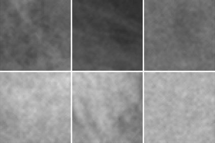
In order to model the different breast density types (fatty and dense), we manually extract a subset of M patches of size N × N pixels. Figure 4 illustrates three different examples of fatty and dense patches. These patches are used as input data for training a classifier, which later on is used to segment new mammograms. To perform the training and the modelling of both fatty and dense tissue, we select the same number of patches representing both tissue types. We will provide more details on this aspect in the experimental section.

Fig 4.

Patch samples. The upper row shows three fatty tissue patches, while the bottom row shows three dense tissue patches.

As mentioned in “Introduction”, we study two different statistical strategies for creating our models: (1) based on the Karhunen–Loeve transform and (2) based on LDA.

Karhunen-Loeve-Based Model (PCA)

This strategy is mainly based on the eigenfaces solution proposed by Turk and Pentland for the face recognition problem.²⁰ The Karhunen–Loeve transform is used in order to reduce the dimensionality of the problem, finding the subset of vectors that best account for the distribution of the training images (our M patches) within the entire image space.

The first step of this process consists in representing each image x_i of the training database as a vector of length N². Afterwards, μ is computed as the mean image of all training images:

1

and the total scatter matrix S_T:

2

In this framework, a linear transformation mapping the original image space into a new feature space is defined as:

3

being W a matrix of size P × N², where P is the number of vectors of the new subspace (P < M). In PCA, the projection is chosen to maximise the determinant of the scatter matrix of the projected samples:

4

being w_i the set of P eigenvectors corresponding to the P largest eigenvalues (called eigenfaces in the original work of Turk and Pentland²⁰). Note that these eigenvectors define the maximum scatter subspace of the original image space. Afterwards, each training image can be transformed into this space by using Eq. 3. In our process of modelling the tissue patches, the result of this transformation is a vector of weights (z_i) per patch i describing the contribution of each eigenvector in representing the corresponding input patch. The set of M weight vectors, z₁... z_m, forms our model. Thus, when a new patch has to be tested, we perform a classification process assigning the patch to the most similar class. As in the original algorithm of Turk and Pentland, the similarity is computed using the nearest neighbour algorithm.²⁰

Linear-Discriminant-Based Model (LDA)

An important aspect of the PCA approach is that the scatter maximised is due not only to the between-class scatter but also to the within-class scatter. Therefore, we also test in this study the behaviour of a linear-discriminant-based strategy,²¹ which is able to tackle this point.

In the LDA framework, the between-class scatter (the dispersion among each class means) is defined as:

5

where C is the number of classes of the training database (in our work C = 2: fatty or dense), μ_k is the mean image of each class C_k and M_k is the number of images in the training database belonging to class C_k. The within-class scatter (the overall sum of the dispersion inside each class) is defined:

6

The aim of LDA is to find the subspace where the between-class scatter is maximised while the within-class is minimised. Formally,

7

where W_PCA is defined by Eq. 4 and W_FLD:

8

Note that this W_FLD definition is necessary in order to avoid the singularities of the within-class scatter matrix.

As in the PCA strategy, each training patch can be transformed into this subspace obtaining a new vector of weights (z_i), which describes the contribution of each vector in representing the patch. Hence, when classifying a new patch, this is projected onto that subspace and classified according to the most similar class using again the nearest neighbour algorithm.

Segmenting the Breast

Once a model is built using either the PCA or LDA strategy, we are ready to classify each pixel of the mammogram as belonging to fatty or dense tissue. For such a task, we open a search window of size N × N centred at each pixel, and we use this patch as the input for the model. Hence, the patch is spanned to the corresponding subspace, and the weights of its components are the input data used in the nearest neighbour algorithm to provide the classification. The result after repeating this simple procedure for all the breast pixels is the final breast segmentation in either fatty or dense class.

Results

This experimental section is divided in two subsections. Firstly, we present a quantitative analysis of the results on the Trueta database using PCA and LDA modelling strategies, analysing also the effect of changing the parameters: (M) the number of patches and (N) the patch size. Afterwards, we present an extensive qualitative validation using both the Trueta and the MIAS database. Notice that we could not use the public MIAS database for a quantitative analysis since the density tissue ground truth is not available.

It is important to remark that the patches used in the modelling step are extracted individually from each database. Observing Figures 1 and 2, one can clearly notice that the tissue appearance of both databases is different. This is due to the fact that the MIAS database was obtained by scanning film screen mammograms, while the Trueta one is full-field digital. Therefore, our modelling process is independently performed for both databases.

The results presented in this paper have been obtained following a ten-folder cross-validation methodology. Hence, each database was divided into ten different groups, containing approximately the same number of mammograms. From each group we extracted a set of patches, containing fatty and dense tissue types. In particular, six fatty and six dense patches were manually selected for each group. Afterwards, nine of the groups were merged and used for doing the training (54 fatty and 54 dense patches for the training), while the mammograms of the remaining group produced the segmentation testing set. This procedure was repeated until all groups were used for testing. Note that using this methodology, each mammogram appears in the test set only once and it is tested using patches extracted from other mammograms.

Quantitative Results

The data used in this analysis is a subset of 60 MLO mammograms of the Trueta database from where dense area was accurately segmented by two radiologists. Hence, we can quantitatively compare both automatic and manual segmentations using PCA and LDA strategies.

The three following measures are used to evaluate the results:

• Accuracy or percentage of correct classification (M1). This measure computes the correct classification of all pixels as being classified as fatty or dense tissue. In terms of True Positives (TP), True Negatives (TN), False Positives (FP), and False Negatives (FN), the M1 measure is computed as:

  9
• Area overlap (M2). This measure only takes dense pixels into account. Being A one segmentation and B the other one, (M2) is defined as the ratio between the number of pixels in the intersection of both segmentations and the number of pixels in the union:

  10
• Dice coefficient (M3).²² This is a common measure in medical imaging that is close to the area overlap. This measure gives more weight to those pixels correctly classified as dense in both segmentations:

  11

Note that all these measures are equal to 1 when both segmented areas are identical, equal to 0 when both areas do not intersect, and have values between 0 and 1 otherwise.

Table 2 shows the obtained results when modelling the breast using the PCA and the LDA strategy. Note that the overlap between both manual and automatic annotations is high, showing a good performance of our approach in all three measures. Observe also that the PCA strategy provides the best results, although the difference is not statistically significant. This is a surprising result because we expected the LDA modelling strategy to have better performance than the PCA one, since it takes the between and within-class scatter of the data into account. However, LDA results in many disconnected dense regions, while the PCA approach provides a more compact classification.

Table 2.

Results of the Proposed Strategies in Terms of Accuracy (M1), Area Overlap (M2) and Dice Coefficient (M3)

	PCA strategy	LDA strategy
M1	0.916 ± 0.038	0.890 ± 0.031
M2	0.900 ± 0.122	0.842 ± 0.196
M3	0.943 ± 0.077	0.876 ± 0.139

One of the advantages of our approach is the small number of parameters required: M the number of patches and N the patch size. The results shown in this paper were obtained using a total number of 54 patches per training of size 50 × 50 pixels. Both parameters were empirically validated and were those which provided a good compromise between the performance of the method and the complexity of the model. Note that the selected number of patches should be large enough to provide sufficient data variation per each tissue class but small enough to avoid overfitting the classifier. On the other hand, when using large patch sizes, our approach provided more homogeneous regions, while when using small sizes, it provided small unconnected regions. This is due to the fact that cumuli of ducts are considered as being part of the dense tissue. It is important to remark that if the patch size is too large, the approach may produce oversegmented results.

Qualitative Results

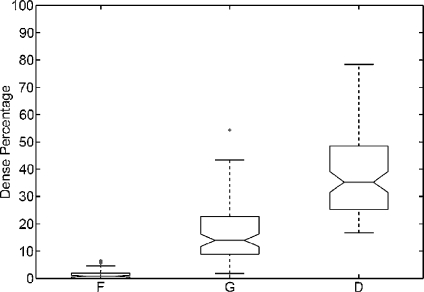
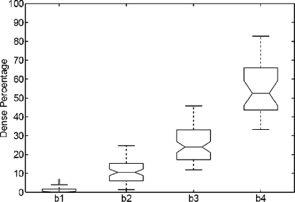
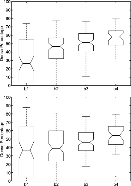
In order to perform a qualitative analysis, we use the PCA modelling strategy (which provided better quantitative results, see Table 2) to obtain the breast segmentations. The qualitative analysis is given in terms of boxplots,²³ a graphical statistical summary of the data. The boxplot is defined by the lower and upper quartiles, while the line inside the box defines the median. The notch represents a robust estimate of the uncertainty about the medians for box-to-box comparison. Hence, boxes whose notches do not overlap indicate that the medians of the groups differ at the 5% significance level. The whiskers are lines that show the extent of the rest of the data, extending from each end of the boxes to the most extreme data value within 1.5*IQR, where IQR is the interquartile range of the sample. Outliers are data with values beyond the ends of the whiskers.

MIAS Qualitative Results

A qualitative analysis is performed using the entire MIAS database (322 images in total). After segmenting the breast in both fatty and dense tissues, we computed the percentage of segmented dense area relative to the overall breast area (fatty and dense areas). Afterwards, we constructed a boxplot analysis detailing this percentage according to each density class provided in the MIAS annotations (fatty, glandular and dense). This is shown in Figure 5. Observe that the percentage of dense area increases according to the class density. Note also that mammograms belonging to fatty class do almost not show any dense area, while dense mammograms have large percentage dispersion. Notice that we obtained several outliers in the fatty and glandular classes. This is due to the fact that there is a small set of mammograms brighter than the rest, and in this cases, the algorithm is not able to correctly recognise the fatty tissue. In these cases, a previous grey-level normalisation of the image should be necessary.²⁴

Fig 5.

Boxplot of breast dense percentage using the MIAS database and its own annotations (F, G and D stand for fatty, glandular and dense class, respectively). The box in the fatty class is almost all over the x-axis.

We repeated the same analysis but using the annotations provided by the radiologists, who classified the MIAS database according to the BIRADS standard. The results are shown in Figure 6. Note that the dense area of mammograms belonging to BIRADS I is again insignificant, while mammograms belonging to BIRADS II have a small part of dense tissue. The dispersion in dense classes is now reduced, and the outliers have also been reduced. Moreover, according to the notches, the difference in the median of all classes is clearly significant.

Fig 6.

Boxplot of breast dense percentage using the MIAS database and the annotations provided by the experts (b1, b2, b3 and b4 stand for BIRADS I, BIRADS II, BIRADS III and BIRADS IV, respectively). The box in the BIRADS I class is almost all over the x-axis.

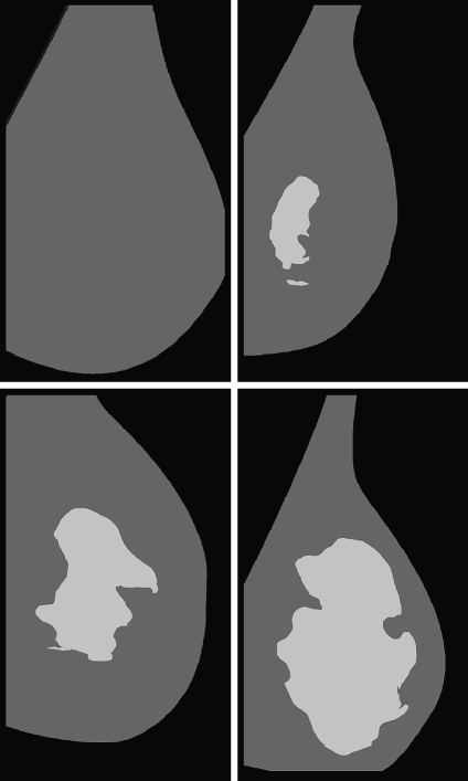
Figure 7 shows the mammogram samples of Figure 1 after applying our segmentation approach using the PCA modelling. The lighter cluster shows the dense area, while the darker one shows the fatty tissue. Note that the dense area of the mammograms is segmented in a single and homogeneous region, except for the mammogram belonging to BIRADS II who has a second small dense cluster. Moreover, observe that the size of the dense cluster increases as the density of the breast also increases.

Fig 7.

Segmentation results using our approach with PCA modelling for the four mammograms of Figure 1.

Trueta Qualitative Results

In this section, we repeat the same qualitative analysis but using the Trueta database and now analysing 125 MLO and 125 CC views independently. The pre-processing step of CC mammograms did not include the pectoral muscle removal since the muscle was not present in this view.

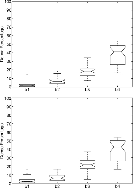
Figure 8 shows the boxplots of the dense percentage obtained. The first row analyses the CC mammograms, while the second one analyses the MLO ones. Note that, in both cases, the percentage increases according to the BIRADS classes. However, we found two outliers using the CC set and two more when using the MLO one. Note that the trend is similar when comparing both datasets, showing that our approach is able to correctly segment both MLO and CC mammograms.

Fig 8.

Boxplot of the dense percentage using the Trueta database. First row using the test set of 125 CC mammograms, while second one using the 125 MLO ones.

Comparing the obtained results using the MIAS and the ones using the Trueta database, we observe that the BIRADS I distribution is better defined when using the former database. This is due to the different nature of the databases. Remember that the MIAS is a digitised database, while the Trueta one is fully digital. In the Trueta database, almost all fatty mammograms have a small region segmented due to the fact that the digital database has more contrast than the digitised one (see for instance Figures 1 and 2). Hence, some ducts and linear structures that are brighter than the fatty breast tissue are incorrectly segmented. In contrast, the performance for the other classes is similar.

Discussions

In order to show the benefits of our approach, we compared the obtained results with a thresholding approach. As already said in “Introduction”, thresholding is one of the most used approaches for breast density segmentation. In particular, we apply here two different well-known thresholding techniques: the first one based on the maxim-entropy thresholding²⁵ and the second one based on the Ridler–Calvard algorithm.²⁶

Figure 9 shows the results obtained for the MIAS database when using both thresholding approaches for breast density quantification. Note that the performance of both thresholding algorithms for class BIRADS I is not the expected one, obtaining a large dispersion in the dense percentage ratio. The reason for this behaviour is that there is a set of mammograms correctly segmented (without dense cluster or being small), while there is another set incorrectly segmented. In these cases, the thresholding approaches segmented the outer part of the breast from the inner part due to the fact that pixels near the skin-line (those with less breast tissue) are darker than the other ones. Hence, in homogeneous fatty mammograms, this tends to produce an incorrect estimation of the threshold. In contrast, the rest of BIRADS classes show more compact results, increasing the median of the class according to the increasing density. However, comparing these results with those shown in Figure 6, the median is higher. This is also a consequence of bad threshold estimation. However, in this case, the bias is smaller due to the fact the tissue of the mammograms is more heterogeneous, and therefore, the estimated threshold is greater than the obtained when segmenting mammograms belonging to BIRADS I.

Fig 9.

Boxplot of breast dense percentage using the MIAS database and two well-known thresholding approaches. First row shows the results using the maximum-entropy thresholding,²⁴ while second one using the Ridler–Calvard algorithm.²⁵

We also want to briefly discuss the performance of the initial pre-processing step explained in “Initial Pre-processing Step”, which was performed in order to remove background, annotations and pectoral muscle of the images. In general, the performance of these algorithms is good enough in most of the cases. However, for the MIAS database, there is a small set of images where the breast segmentation algorithm decreases its accuracy, incorrectly segmenting a small border of the breast. In contrast, regarding the Trueta database, the pectoral muscle is incorrectly segmented in few cases, having the problem of segmenting a small portion of fatty tissue besides the pectoral muscle. However, in both cases, the segmentation algorithm segments correctly the dense tissue due to the fact that the algorithm does not depend on the fatty tissue. Note that, for these special situations, as a small area of the fatty tissue has been suppressed, the ratio of dense area is slightly biased to higher values.

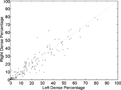
A different way of showing the robustness of our approach is to compare the left and right mammograms. From a medical point of view, this is justified by the fact that both breasts of the same woman have similar internal tissue.²⁷ Note that we can perform this analysis because the MIAS database is composed by left and right mammograms of 161 women.

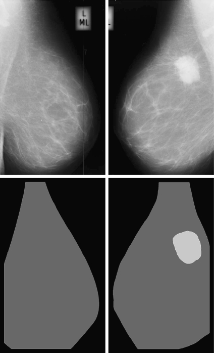
In Figure 10, we show the dense percentage plot of the right mammograms versus the dense percentage of the left mammograms. We also include the diagonal line to show the ideal case. According to the figure, most of the mammograms are segmented in a similar way. However, it is difficult to follow the ideal case. This is due to the segmentation algorithm and also to the internal tissue (although being similar is not identical). In fact, some of the discrepancies are due to the presence of different tissue or abnormalities in one of the breast. In this sense, the first row of Figure 11 shows a pair of left–right mammograms of the same patient. Observe that the right mammogram has a large white region being a big mass. The second row of the figure shows the result of segmenting each mammogram using our approach. Note that the presence of the mass biased the algorithm, which detected the mass as a cluster of dense tissue. Obviously, the comparison of left–right mammograms in these cases does not follow the ideal case.

Fig 10.

Bilateral analysis: each dot marks the left and right dense percentage of each mammogram pair.

Fig 11.

Segmentation results of a left and right mammogram pair. The large mass in the right mammogram is incorrectly segmented as being dense tissue.

Conclusions

A statistical approach to model and segment the mammograms according to their internal density has been presented. The algorithm learns the characteristics and the variability of the different tissue, being able to correctly segment the breast into fatty and dense regions. Moreover, two different breast modelling strategies have also been compared. The segmentation approach is quantitatively and qualitatively evaluated using two different databases, obtaining better results with the PCA strategy. Furthermore, the obtained results show the feasibility and robustness of our approach.

The final goal of our research is directed to the use of fatty and dense information to recover the 3D internal structure of the breast by correlating both tissue segmentations of CC and MLO views.

References

- 1.American Cancer Society: Breast Cancer: Facts and Figures, 2003–04. Atlanta: ACS, 2003
- 2.Australian Institute of Health and Welfare & National Breast Cancer Centre: Breast cancer in Australia: an overview. Cancer series. Canberra: AIHW, 2006, p. 34
- 3.R2 ImageChecker. http://www.r2tech.com. Accessed 1 January 2007
- 4.iCAD Second Look. http://www.icadmed.com. Accessed 1 January 2007
- 5.Ho WT, Lam PWT. Clinical performance of computer-assisted detection (CAD) system in detecting carcinoma in breasts of different densities. Clin Radiol. 2003;58:133–136. doi: 10.1053/crad.2002.1131. [DOI] [PubMed] [Google Scholar]
- 6.Obenauer S, Sohns C, Werner C, Grabbe E. Impact of breast density on computer-aided detection in full-field digital mammography. J Digit Imaging. 2006;19(3):258–263. doi: 10.1007/s10278-006-0592-x. [DOI] [PMC free article] [PubMed] [Google Scholar]
- 7.Brem RF, Hoffmeister JW, Rapelyea JA, Zisman G, Mohtashemi K, Jindal G, DiSimio MP, Rogers SK. Impact of breast density on computer-aided detection for breast cancer. Am J Roentgenol. 2005;184(2):439–444. doi: 10.2214/ajr.184.2.01840439. [DOI] [PubMed] [Google Scholar]
- 8.Wolfe JN. Risk for breast cancer development determined by mammographic parenchymal pattern. Cancer. 1976;37:2486–2492. doi: 10.1002/1097-0142(197605)37:5<2486::AID-CNCR2820370542>3.0.CO;2-8. [DOI] [PubMed] [Google Scholar]
- 9.Freixenet J, Oliver A, Martí R, Lladó X, Pont J, Pérez E, Denton ERE, Zwiggelaar R. Eigendetection of masses considering false positive reduction and breast density information. Med Phys. 2008;35(5):1840–1853. doi: 10.1118/1.2897950. [DOI] [PubMed] [Google Scholar]
- 10.Boyd NF, Byng JW, Jong RA, Fishell EK, Little LE, Miller AB, Lockwood GA, Tritchler DL, Yaffe MJ. Quantitative classification of mammographic densities and breast cancer risk: results from the Canadian national breast screening study. J Natl Cancer Inst. 1995;87:670–675. doi: 10.1093/jnci/87.9.670. [DOI] [PubMed] [Google Scholar]
- 11.Sivaramakrishna R, Obuchowski NA, Chilcote WA, Powell KA. Automatic segmentation of mammographic density. Acad Radiol. 2001;8(3):250–256. doi: 10.1016/S1076-6332(03)80534-2. [DOI] [PubMed] [Google Scholar]
- 12.Ferrari RJ, Rangayyan RM, Borges RA, Frere AF. Segmentation of the fibro-glandular disc in mammograms via Gaussian mixture modelling. Med Biol Eng Comput. 2004;42:378–387. doi: 10.1007/BF02344714. [DOI] [PubMed] [Google Scholar]
- 13.Aylward SR, Hemminger BH, Pisano ED: Mixture modelling for digital mammogram display and analysis. Int Work Dig Mammography 305–312, 1998
- 14.Saha PK, Udupa JK, Conant EF, Chakraborty P, Sullivan D. Breast tissue density quantification via digitized mammograms. IEEE Trans Med Imag. 2001;20(8):792–803. doi: 10.1109/42.938247. [DOI] [PubMed] [Google Scholar]
- 15.Zwiggelaar R, Denton ERE: Optimal segmentation of mammographic images. In Int Work Dig Mammography 751–757, 2004
- 16.Petroudi S, Brady M. Breast density segmentation using texture. Lect Not Comp Sc. 2006;4046:609–615. doi: 10.1007/11783237_82. [DOI] [Google Scholar]
- 17.Suckling J, Parker J, Dance DR, Astley SM, Hutt I, Boggis CRM, Ricketts I, Stamatakis E, Cerneaz N, Kok SL, Taylor P, Betal D, Savage J: The Mammographic Image Analysis Society digital mammogram database. Int Work Dig Mammography 211–221, 1994
- 18.Martí R, Oliver A, Raba D, Freixenet J. Breast skin-line segmentation using contour growing. In Lect Not Comp Sc. 2007;4478:564–571. doi: 10.1007/978-3-540-72849-8_71. [DOI] [Google Scholar]
- 19.Kwok SM, Chandrasekhar R, Attikiouzel Y, Rickard MT. Automatic pectoral muscle segmentation on mediolateral oblique view mammograms. IEEE Trans Med Imag. 2004;23(9):1129–1140. doi: 10.1109/TMI.2004.830529. [DOI] [PubMed] [Google Scholar]
- 20.Turk MA, Pentland AP. Eigenfaces for recognition. J Cogn Neurosci. 1991;3(1):71–86. doi: 10.1162/jocn.1991.3.1.71. [DOI] [PubMed] [Google Scholar]
- 21.Belhumeur PN, Hespanha JP, Kriegman DJ. Eigenfaces vs Fisherfaces: Recognition using class specific linear projection. IEEE Trans Pattern Anal Mach Intel. 1997;19(7):711–720. doi: 10.1109/34.598228. [DOI] [Google Scholar]
- 22.Dice LR. Measures of the amount of ecologic association between species. Ecology. 1945;26:297–302. doi: 10.2307/1932409. [DOI] [Google Scholar]
- 23.McGill R, Tukey JW, Larsen WA. Variation of boxplots. Am Stat. 1978;32:12–16. doi: 10.2307/2683468. [DOI] [Google Scholar]
- 24.Snoeren PR, Karssemeijer N. Gray-scale and geometric registration of full-field digital and film-screen mammograms. Med Image Anal. 2007;11(2):146–156. doi: 10.1016/j.media.2006.11.003. [DOI] [PubMed] [Google Scholar]
- 25.Pun T. Entropy thresholding: a new approach. Comput Vis Graph Image Process. 1981;16:210–239. doi: 10.1016/0146-664X(81)90038-1. [DOI] [Google Scholar]
- 26.Ridler TW, Calvard S. Picture thresholding using an iterative selection method. IEEE Trans Syst Man Cybern. 1978;8(8):629–632. [Google Scholar]
- 27.Kopans D. Breast Imaging. Philadelphia: Lippincott-Raven; 1998. [Google Scholar]