A Study on the Feasibility of Active Contours on Automatic CT Bone Segmentation

Abstract

Automatic bone segmentation of computed tomography (CT) images is an important step in image-guided surgery that requires both high accuracy and minimal user interaction. Previous attempts include global thresholding, region growing, region competition, watershed segmentation, and parametric active contour (AC) approaches, but none claim fully satisfactory performance. Recently, geometric or level-set-based AC models have been developed and appear to have characteristics suitable for automatic bone segmentation such as initialization insensitivity and topology adaptability. In this study, we have tested the feasibility of five level-set-based AC approaches for automatic CT bone segmentation with both synthetic and real CT images: namely, the geometric AC, geodesic AC, gradient vector flow fast geometric AC, Chan–Vese (CV) AC, and our proposed density distance augmented CV AC (Aug. CV AC). Qualitative and quantitative evaluations have been made in comparison with the segmentation results from standard commercial software and a medical expert. The first three models showed their robustness to various image contrasts, but their performances decreased much when noise level increased. On the contrary, the CV AC’s performance was more robust to noise, yet dependent on image contrast. On the other hand, the Aug. CV AC demonstrated its robustness to both noise and contrast levels and yielded improved performances on a set of real CT data compared with the commercial software, proving its suitability for automatic bone segmentation from CT images.

Introduction

Along with the advancements in medical imaging modalities, such as ultrasound, magnetic resonance imaging (MRI), and computed tomography (CT), medical image analysis has drastically increased its importance in clinical procedures.¹ Current research works can be classified into four categories according to their purposes: enhancement, registration, visualization, and segmentation of the images. Image enhancement² deals with yielding more accurate images with improved contrast and reduced noise. Image registration³ is an essential technique for multimodality imaging where MRI, single photon emission CT, positron emission tomography, or angiography could be registered to each other to complement information. For instance, the complementary information, such as soft-tissue information from MRI, could be added to CT or vascular data to the anatomical MRI. Image visualization⁴ is used to provide more effective viewing of complex structures or information of the human body. Image segmentation deals with an extraction of targeted regions of interest from the original image with minimum human interaction. Nowadays, due to increasing computing power, a combination of these research topics is integrated into the computer-aided surgery planning or the image-guided surgery system.¹

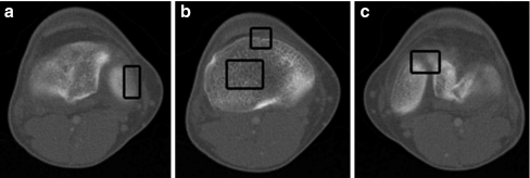
In computer-assisted orthopedic surgery, automatic image segmentation, especially automatic bone segmentation from CT imagery, is a critical but challenging component. The challenges are twofold: in developing good segmentation algorithms and in automating them. The former has three main hindrances: (1) inhomogeneous bone structures, (2) low-contrast edges, and (3) overlapping intensity values of bones, whereas the latter is even more challenging because it requires high performance to be obtained with minimal user interactions, such as image-dependent initialization or prior information about the number of bones and/or their shapes. Inhomogeneous regions are due to the nature of the bone structure in which the outer layer (i.e., cortical bone) is denser than the inner one (i.e., spongy bone). As a result, the cortical bone appears brighter in CT images while the spongy bone is darker and sometimes textured. Moreover, during the image acquisition process, small gaps can exist in the bone surfaces where blood vessels go through. Also, when the boundaries of two bone regions are close to each other, they tend to be diffused, making the background pixels between them brighter and, thus, lowering contrast. The boxes in Figure 1 indicate these challenging characteristics.

Fig 1.

Typical CT bone images with challenging obstacles for accurate segmentation such as a weak edges, b gaps and texture areas, and c blurred interbone regions as indicated with boxes.

There have been several attempts, including global thresholding, region growing,⁵ region competition,⁶ atlas-based,⁷ artificial intelligence, watershed segmentation approaches, and various combinations thereof, as surveyed in.^8,9 Most of the methods have shown success in certain anatomical structures where they have been optimized, such as carpal bones,⁹ acetabulum and femoral head,¹⁰ spinal canal,¹¹ pelvis,^7,12 vertebrae,¹³ ribs,¹⁴ and phalanx bones.¹⁵ In,⁸ two methods were validated on knee bone segmentation, which is also the subject of this study. The first one was a four-step process¹⁶ that contains region-growing using local adaptive thresholds, discontinued-boundary closing, anatomically oriented boundary adjustment, and manual correction. The other one was a seeded edge-detection and tracing algorithm¹² where initial seeds were obtained by thresholding in intensity histograms. The aforementioned methods often require several steps with certain degrees of user interaction; additional tasks are especially needed to close discontinued object boundaries.

On the other hand, since it was first introduced by Kass et al.,¹⁷ the deformable curve or snake or active contour (AC) model has attracted much attention in the image segmentation research community. In general, AC models are the descriptions of contours in 2D or surfaces in 3D that evolve under an appropriate energy to move toward desired features, such as object boundaries. One advantage of these models is that they are always closed, yielding continuous object boundaries, which no longer requires postprocessing tasks to connect discontinued ones. However, because their performance depends heavily on the initial contour and image noise, many modified versions have been proposed to cope with bone segmentation. In,¹⁸ the authors incorporated region-based image features to the snakes model of Kass et al.,¹⁷ which was edge-based, to improve its convergence and dependence on initial position and to reduce its sensitivity to noise. Sharing the same idea, Pardo et al.,¹⁹ introduced new region potential term that did not rely on prior knowledge about image statistics. Although the integration of edge and region information made the model more robust to noise and permitted a more precise segmentation of bones, the automatic selection of relative weighting between edge and region terms remains an unsolved problem. In another work,⁹ Sebastian et al. combined conventional approaches, such as bubble ACs,²⁰ region growing, region competition, and morphological operations, in a unified framework. Specifically, from initialized seeds, region growing took place under the evolution implementation of bubbles. The growth of seeds was also modulated by the interseed skeleton-mediated competition between neighbor regions. The method inherited the advantages of each individual approach to overcome the discretization drawbacks of the region competition method, the convergence problems, and initial placement sensitiveness of curve evolution methods. Nevertheless, it had limited performance in the case of narrow and diffused interbone spaces. Ballerini and Bocchi²¹ proposed the use of multiple genetic snakes whose energy minimization was based on the genetic algorithms, which helped to tackle the initialization problem. However, the method required much user interaction in determining the energy weights and the functionals governing the snake behavior.

Although those modified AC models can overcome the drawbacks of conventional ones in some particular situations, they are still far from the automatic bone segmentation procedure that requires high accuracy, initialization insensitivity, and topology adaptability (i.e., automatic splitting and merging ability to capture multiple objects). In this study, we evaluate five recently developed AC models, namely, the geometric AC,²² the geodesic AC,²³ the gradient vector flow (GVF) fast geometric AC²⁴ (GVF-Geo AC), the Chan–Vese (CV) AC,^25,26 and the density distance augmented CV AC (Aug. CV AC), which was developed by us,²⁷ in extracting knee bones from CT images in comparison against 3D-DOCTOR software,¹ which is considered as a semiautomatic method. We do not consider other models that incorporate prior knowledge about object shape^28,29,30 or texture³¹ since they require a training stage and, thus, are hardly automated and cannot be fairly compared. Our motivation here is to find the most appropriate technique that produces the highest segmentation accuracy with the least amount of user interaction. From a clinical perspective, the development of such an algorithm is of great value since it can significantly reduce the amount of time a practitioner spends on inspecting and modifying the results of a more-or-less automatic segmentation. Knee bones are chosen as the region of interest because they have all the segmentation challenges described above. Together with both qualitative and quantitative evaluations on real CT images, the influences of noise and contrast are also investigated with simulated data. Our evaluation results indicate that the Aug. CV AC model produces superior segmentation results with strong feasibility for automatic bone segmentation.

Materials and Methods

AC Models

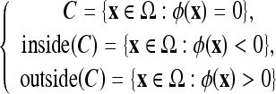
The five models used in this study are geometric-type ACs, which are based on the theory of curve evolution³² and the level-set framework.^33,34 In this framework, the curve C is implicitly represented by the zero-level set of a Lipschitz function , which is usually defined as a signed distance function such that

1

where is the image plane. The main idea is to evolve the embedding function ϕ and keep track of its zero-level set. The function ϕ moves up and down on a fixed coordinate system without changing its topology, but its zero-level set corresponding to the contour C may split or merge. This is an advantage of level-set-based ACs since their topology is naturally handled to capture multiple objects without additional efforts. In general, the evolution is performed using three forces: one internal force (curvature-based) and two external forces (normal direction and vector-field-based) as follows.

2

where κ is the Euclidean curvature and b, V_N, and are three parameters determining the velocity and direction of the evolution. The curvature-based force smoothes the curve, the normal-direction force shrinks or expands the curve along its normal direction, and the external vector-field-based force acts as a translation operator. Depending on how those three parameters are chosen, we have different AC models as listed below.

(Original) Geometric AC

The (original) geometric AC^22,35 was proposed using an edge-based function g(x), which approaches zero on the edges and one in other regions, e.g., , where σ_e is a scaling factor and is the convolution of the input image I with a Gaussian kernel . The evolution flow is

3

where V₀ is a real constant, meaning that the curve is shrunk or expanded at a constant velocity. The product g(κ + V₀) determines the overall evolution speed of level sets of ϕ(x,t). The geometric AC is derived, not by an energy minimization, but by a curve evolution method where a constant normal direction force is used together with an edge-based function g to evolve and stop the curve on the object boundaries.

Geodesic AC

The geometric AC works well, in general, for objects that have good contrast. If there are weak edges and/or gaps along edges, however, it tends to pass through these areas because gradient values are not large enough for g(x) to approach zero. To overcome this limitation, the following evolution flow, called geodesic AC flow, was introduced in^23,36 and can be expressed as

4

Different from the geometric AC, which has no energy minimization, this model is derived from the problem of finding a curve of minimal weighted length, which was proven to be equivalent to a particular case of the energy of the snakes model.¹⁷ Comparing this with the previous model (Eq. 3), we see that the extra stopping term is used to increase the attraction of the evolving contour toward weak boundaries because points to the middle of the edges. By this way, the curve can stop on the boundaries even when g ≠ 0.

Gradient Vector Flow Fast Geometric AC

The GVF³⁷ refers to a slowly varying and bidirectional vector field that is nearly the same as the gradient of an image in the neighborhood of the boundaries (where the gradient magnitude is large) and still has significant values in the homogeneous regions (where the gradient gets close to zero) via a diffusion process. One can think of this field as the optimal direction to be followed to reach the object boundaries. Inspired from that observation, Paragios et al.²⁴ proposed an integration of GVF into the geometric AC as follows:

5

where is the normalized GVF and with N(x) as the inward normal of the curve and δ as a scaling factor (chosen as δ = 1 in our implementations). K(x) approaches one when the normal and the GVF are close to orthogonal and zero otherwise.

In the above flow, has the effect of a bidirectional flow that moves the curve toward object boundaries from either side, whereas V₀K(x) serves as an adaptive balloon force used to determine the evolution when the bidirectional flow term becomes inactive. Similar to that of the geometric AC, the overall speed of this curve evolution is coupled with the edge-driven information via the stopping term g. The GVF-Geo AC replaces in the geodesic AC (Eq. 4) with the GVF. This increases the capture range due to the slowly varying characteristic of the GVF.

CV AC

Chan and Vese²⁵ proposed an alternative form of AC based on the Mumford and Shah functional for segmentation.³⁸ Unlike other level-set-based ACs, which rely much on the gradient of the image as the stopping term and, thus, have unsatisfactory performance in noisy images, the CV AC model instead utilizes the homogeneity characteristic of an object. In this case, the image I is assumed to consist of two areas with approximately piecewise-constant intensities, of different values c_in and c_out. The “fitting” term is defined as

6

where c_l and c₂ are, respectively, the average intensities inside and outside the variable curve C. As can be seen in Figure 2, the “fitting” term is minimized if the curve C is placed exactly on the boundary of the two areas.

Fig 2.

All possible positions of the curve. When it is on the boundary of the object, the “fitting” term is minimized.

One can regularize the solution by constraining the length of the curve and the area inside it. Then, the level set formulation of this model is expressed as

7

where ν and V₀ are adjustment constants. Like the geometric AC flow, the CV AC flow does not have an external vector-field-based force, reducing the computational cost. This flow evolves the AC, looking for a two-phase segmentation of the image, given by , where H is the Heaviside function

8

Density Distance Augmented CV AC

Compared to other AC models, the CV AC can detect the boundaries more exactly since it does not need to smooth the initial image (via the edge function g), even if it is very noisy. This model was also shown to provide a relaxed initial position requirement. However, the convergence of the CV AC depends on the homogeneity of the segmented objects. When the objects are largely inhomogeneous, such as carpal bones or knee bones in CT images, the CV AC provides unsatisfactory results. To overcome this limitation, we have recently proposed a novel model, called the Aug. CV AC.²⁷ The proposed model searches for the solution that not only minimizes the dissimilarity within each segment (which is what the CV AC does), but also maximizes the distance between different segments. In this regard, we used the Bhattacharrya distance as the distance measure for its simple analytical form and its better performance in signal selection.³⁹ The evolving flow was given as

9

with

10

where is a weighting constant (we choose β = 0.5 in all experiments) and A_in, A_out, p_in, and p_out, respectively, are the areas and the density functions inside and outside the curve C, given by

11

12

is a certain image feature (intensity, color, texture, etc.) and is the Bhattacharyya coefficient.³⁹ More details of the Aug. CV AC are available in.²⁷

Parameter Setting and Tuning

There are four parameters for the above-mentioned AC models: σ, σ_e, V₀, and ν. σ determines the width of the smoothing Gaussian kernel used in the edge function g and is chosen small enough to retain minute details. It is fixed as σ = 0.3 for all experiments. The rest are chosen depending on each specific case. Decreasing σ_e helps to detect weak edges but, in turn, traps the contour in false edges that are caused by noise. Since V₀ constantly moves the contour along its normal direction regardless of its current position, increasing V₀ will speed up the evolution but can march the contour over weak edges. So, σ_e and V₀ should be large for noisy images and vice versa. ν weights the length constraint of the CV and the Aug. CV ACs. If we have to detect all or as many objects as possible and of any size, then ν should be small. If we have to avoid detecting smaller objects (like points, due to noise), then ν has to be larger.

In practice, some preliminary tests are needed for a new set of images with similar characteristics. In our experiments, we estimate the noise and contrast levels of one or two images from a testing set to provide an initial guess of the parameter set based on the above guidelines. Then, we use a coarse-to-fine scheme to obtain the “best” parameters based on both visual evaluation and quantitative measures.

Testing Data

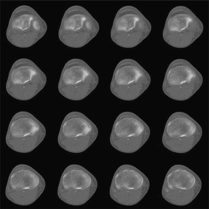
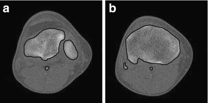
Three testing data sets, named contrast, noisy, and real CT images, are used to test the five techniques on CT bone segmentation. The last consists of 16 CT images covering the knee regions of one person; see Figure 3. These images are selected because they have typical challenges for segmentation, such as inhomogeneous objects, low-contrast edges, and overlapping intensity values, as described in the “Introduction.” The two other data sets are of synthetic data, made to see how these techniques behave at different contrast and noise levels, respectively, and were created as follows: First, we asked a medical expert to carefully extract bone regions from the 16 CT images, which will be used as “ground truths” later on; see Figure 4 for two sample ground truths corresponding to the first and the last images of the set. Then, we placed each extracted bone region on ten homogenous backgrounds with various intensities to obtain ten images having contrast varying from 1% to 20%. Here, we adopt the definition of contrast introduced by Morrow et al.⁴⁰

13

where B and B₀ are, respectively, the mean intensity of the object (foreground) and the surrounding region (background) in an image. In our real CT data, the contrast is about 8%. To our knowledge, CT images with contrasts of 20% are quite clear, and those with contrasts of 1% are beyond the worst case. By this way, we had a contrast data set consisting of 160 images (16 images × ten contrast levels each) with typical CT bone segmentation challenges. Similarly, placing extracted bones on noisy backgrounds with signal-to-noise ratios (SNR) of 50, 40, 30, 20, and 10 dB, we formed a noisy data set consisting of 80 images (16 images × five noise levels each). Here, Gaussian noise was used for its simplicity and popularity.^12,16 Images with SNRs of 10 dB are beyond the worst case. The difference between our synthetic images and real CT images is that the former has a synthetic background such that its contrast and noise levels can be controlled.

Fig 3.

Real CT data set.

Fig 4.

Bone regions delineated by a medical expert, used as ground truths.

Evaluation Method

For quantitative comparison, we use two error measures, ε₁ and ε₂, defined as

14

where # denotes the number of points in a set and Hd(A,B) denotes the Hausdorff distance between two polygons A and B.

15

where and dist(a,b) is the Euclidean distance between points a and b.

The error measure ε₁ quantifies the relative overlap between the segmented and the true regions and measures the difference of the extracted and the true contours. The former provides a global goodness of the result, whereas the latter determines how much detail of the object shape is captured. The closer these measures are to zero, the better the segmentation is.

Experimental Results and Discussions

In this section, we first analyze the topology-adaptability and initialization-insensitivity characteristics of the five AC models. Then, their robustness to various contrast and noise levels will be investigated. Finally, their performances on the real CT data set are evaluated in comparison with that of the 3D-DOCTOR software. The AC models are implemented using MATLAB®. Parameters of each model are first selected using the guidelines in the section “Parameter Setting and Tuning” and will be specified in each case. Then, the contours evolve automatically under forces determined by the image itself without any further user interaction. The evolution is an iterative process and stops when the contours in two consecutive iterations are the same (i.e., unchanged).

Topology Adaptability and Initialization Insensitivity

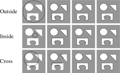
We consider an AC to be topology-adaptable if it can naturally split and merge to capture multiple objects in the image without any prior information and initialization-insensitive if it can do that regardless of its initial position and size. Figure 5 shows three types of initialization and the corresponding results. Note that only one representative result is shown for three models, geometric, geodesic, and GVF-Geo AC, because they yield similar results for this synthetic image. We can see that these three models work well with the first two types (the initial contour is totally outside or inside the objects) but fail with the last one (initial contour is across the objects), whereas the CV and the Aug. CV ACs succeeds with all three types. The reason is that the former three models can only move in a fixed direction based on the sign of the constant V₀; see Eqs. 3–5. When V₀ is positive (negative), the whole contour will shrink (expand) all the time. Meanwhile, the image-dependent term in the CV AC flow (Eq. 7) [or ϑ(x) in the Aug. CV AC flow (Eq. 9)] allows the contour to expand and shrink where appropriate because it can be negative at some points and positive at others.

Fig 5.

Topology adaptability and initialization sensitivity. Left to right: initialization, geometric–geodesic–GVF-Geo, CV, and Aug. CV ACs. The latter two models succeed with all three types of initialization, whereas the others fail with the cross-type.

Experiment 1—Performance at Different Contrast Levels

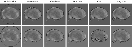
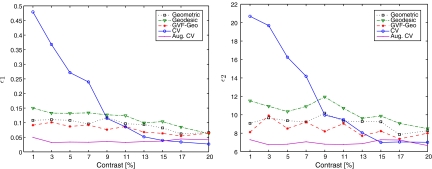
In this experiment, we use the contrast data set to evaluate the performance of the AC models with respect to different contrast levels. The parameter settings are chosen as described in the section “Parameter Setting and Tuning” and shown in Table 1. Figure 6 shows visual results from two samples having contrasts of 13% and 1%, respectively. Mean values of error measures as functions of contrast level are plotted in Figure 7, and corresponding SD values are given in Table 2. We can see that, although the CV AC performs well when image contrast is high (more than 15%), its performance decreases very quickly with the contrast, whereas the others are more robust to contrast level. One possible reason is that the homogeneity assumption of the CV model cannot be guaranteed in low-contrast images, i.e., many parts of the object resemble background and, thus, are likely to be misclassified (see Figure 6, lower row).

Table 1.

Parameter Settings for Experiment 1

Geometric	Geodesic	GVF-Geo	CV (ν, V0)	Aug. CV (ν, V0)
0.2, 0.5	0.2, 0.7	0.2, 0.5	1, 0	1, 0

Fig 6.

Performance at different contrast levels. Upper row: contrast = 13%, and lower row: contrast = 1%. The ground truth is shown in Figure 4b.

Fig 7.

Plots of error means vs contrast level. Mean value is calculated over 16 samples at each contrast level.

Table 2.

Mean and SD of Error Measures for Contrast Data Set

	Contrast [%]	Mean (SD)
		Geometric	Geodesic	GVF-Geo	CV	Aug. CV
	1	0.108 (0.074)	0.150 (0.095)	0.092 (0.029)	0.479 (0.055)	0.050 (0.041)
	3	0.110 (0.082)	0.133 (0.070)	0.101 (0.060)	0.368 (0.159)	0.032 (0.022)
	5	0.108 (0.096)	0.132 (0.077)	0.087 (0.046)	0.271 (0.109)	0.034 (0.024)
	7	0.096 (0.078)	0.134 (0.088)	0.092 (0.079)	0.239 (0.105)	0.033 (0.020)
	9	0.118 (0.105)	0.127 (0.088)	0.076 (0.051)	0.115 (0.080)	0.036 (0.026)
	11	0.096 (0.100)	0.124 (0.109)	0.087 (0.066)	0.086 (0.036)	0.032 (0.024)
	13	0.094 (0.073)	0.099 (0.080)	0.068 (0.038)	0.052 (0.034)	0.035 (0.024)
	15	0.082 (0.070)	0.104 (0.072)	0.063 (0.051)	0.039 (0.023)	0.037 (0.023)
	17	0.062 (0.039)	0.085 (0.054)	0.054 (0.018)	0.034 (0.018)	0.044 (0.029)
	20	0.066 (0.033)	0.063 (0.021)	0.064 (0.042)	0.027 (0.012)	0.041 (0.024)
	1	9.071 (3.472)	11.512 (3.517)	8.121 (1.473)	20.690 (2.410)	7.301 (2.091)
	3	9.672 (3.847)	10.921 (3.395)	9.913 (3.605)	19.682 (4.391)	6.757 (1.763)
	5	9.366 (3.523)	10.357 (3.101)	8.512 (2.792)	16.251 (6.632)	6.819 (1.750)
	7	9.225 (3.074)	10.902 (3.491)	9.204 (3.510)	14.180 (6.770)	7.074 (2.532)
	9	10.184 (4.148)	11.943 (3.828)	8.207 (2.792)	9.975 (6.721)	6.814 (1.806)
	11	9.314 (3.942)	10.711 (4.092)	9.055 (2.866)	9.487 (4.481)	6.783 (1.854)
	13	9.273 (3.021)	9.620 (3.772)	7.714 (2.176)	8.059 (2.234)	6.867 (1.894)
	15	9.247 (3.690)	9.873 (3.403)	8.233 (3.234)	7.006 (1.882)	7.292 (2.243)
	17	7.861 (2.253)	9.074 (3.310)	7.382 (1.817)	7.053 (1.850)	7.261 (2.217)
	20	8.279 (1.893)	8.494 (2.481)	8.009 (2.692)	7.028 (1.861)	6.665 (3.010)

Experiment 2—Performance at Different Noise Levels

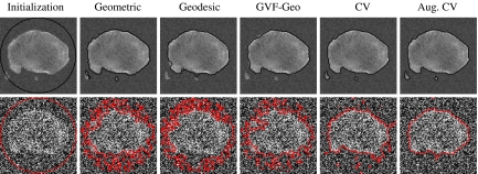
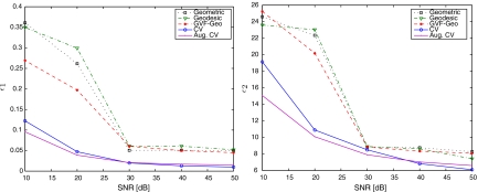
Similarly, the noisy data set is used to evaluate the performance of the five AC models with respect to various noise levels. The parameter settings are shown in Table 3 and sample results in Figure 8. Quantitative comparisons for this testing data set are given in Figure 9 and Table 4. The geometric, the geodesic, and the GVF-Geo ACs provide similar performance to the others when noise level is low. However, they tend to get stuck in false edges caused by noise when noise level increases due to the edge function g. On the other hand, the CV and the Aug. CV are more robust to noise, as they do not depend on the edge information.

Table 3.

Parameter Settings for Experiment 2

SNR [dB]	Geometric	Geodesic	GVF-Geo	CV (ν, V0)	Aug. CV (ν, V0)
10	20, 3	20, 7	30, 7	1, 0	1.5, 0
20	3, 3	3, 9	4, 6	0.5, 0	1, 0
30	1, 1	2, 1	3, 1	0.05, 0	0.5, 0
40	1, 1	2, 1	3, 1	0.05, 0	0.5, 0
50	1, 1	2, 1	3, 1	0.05, 0	0.5, 0

Fig 8.

Performance at different noise levels. Upper row: SNR = 30 dB, lower row: 10 dB. The ground truth is shown in Figure 4b.

Fig 9.

Plots of error means vs SNR. Mean value is calculated over 16 samples at each SNR.

Table 4.

Mean and SD of Error Measures for Noisy Data Set

	SNR [dB]	Mean (SD)
		Geometric	Geodesic	GVF-Geo	CV	Aug. CV
	10	0.361 (0.090)	0.350 (0.087)	0.269 (0.067)	0.122 (0.031)	0.096 (0.024)
	20	0.262 (0.065)	0.299 (0.075)	0.197 (0.049)	0.047 (0.012)	0.039 (0.010)
	30	0.051 (0.013)	0.061 (0.015)	0.061 (0.016)	0.020 (0.018)	0.021 (0.003)
	40	0.051 (0.020)	0.061 (0.011)	0.050 (0.010)	0.013 (0.005)	0.017 (0.007)
	50	0.050 (0.011)	0.052 (0.009)	0.045 (0.012)	0.010 (0.004)	0.015 (0.004)
	10	24.597 (5.402)	23.586 (5.403)	25.237 (5.406)	19.144 (4.785)	15.074 (3.771)
	20	22.347 (5.594)	23.030 (5.594)	20.186 (5.051)	11.903 (3.117)	10.094 (3.270)
	30	8.854 (2.213)	8.902 (2.231)	8.833 (2.362)	8.507 (2.381)	7.906 (2.235)
	40	8.756 (3.217)	8.620 (2.457)	8.339 (3.215)	6.827 (2.103)	7.036 (2.671)
	50	8.282 (3.031)	7.421 (1.543)	8.090 (2.232)	6.102 (2.142)	6.597 (1.328)

Experiment 3—Performance with Real Data

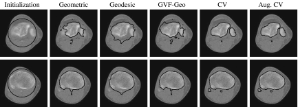
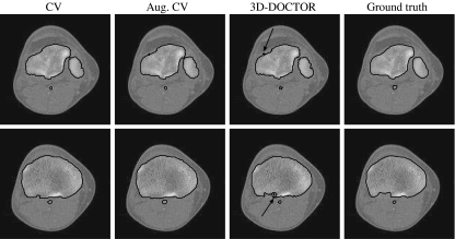
The aim of this experiment is to investigate how the AC models work with real CT images in comparison against 3D-DOCTOR software. The parameter settings are shown in Table 5. Figure 10 shows segmentation results for two sample CT images. It can be seen that the first three models, i.e., the geometric, the geodesic, and the GVF-Geo ACs, do not generate visually satisfactory results, whereas the other two do. The geometric AC tends to pass through some areas in the bone boundary where the stopping function g is not small enough due to weak edges and/or gaps. In this situation, the geodesic AC with the extra stopping term () (Eq. 4) can pull back the boundary-passing-through contour in weak-edge regions, but it is likely to get stuck in false edges caused by noises. The GVF-Geo AC model (Eq. 5) has a similar problem. In contrast, the CV and the Aug. CV AC models can successfully find the bone boundaries. The qualitative comparisons between these two models and the 3D-DOCTOR software are presented in Figure 11. These ACs yield better results in the sense that the contours are smoother and do not contain cross-over parts as the commercial software does.

Table 5.

Parameter Settings for Experiment 3

Geometric	Geodesic	GVF-Geo	CV (ν, V0)	Aug. CV (ν, V0)
0.2, 0.4	0.2, 0.8	0.2, 1.2	0.5, 0	5.0, 0

Fig 10.

Two-sample segmentation results, whose corresponding ground truths are shown in Figure 4. The last two AC models generate visually satisfactory results, whereas the others fail.

Fig 11.

Qualitative comparison with the commercial software. The contours from the 3D-DOCTOR software contain cross-over parts (see the arrows), whereas those from the AC models do not.

The mean and standard deviation of the error measures for 16 images are given in Table 6. Among the five AC models, the last two perform well, and their performance is comparable to that of the 3D-DOCTOR software. The smaller value of these models over the commercial software can be explained by the better boundary shapes they yielded.

Table 6.

The Mean and SD of Error Measures of AC Models and the 3D-DOCTOR Software Performed on 16 CT Images

	Geome.	Geode.	GVF-Geo.	CV	Aug. CV	3D-DOCTOR
	0.184 (0.078)	0.155 (0.078)	0.147 (0.068)	0.086 (0.016)	0.089 (0.013)	0.078 (0.012)
	12.741 (3.240)	10.846 (3.924)	11.623 (3.313)	6.764 (1.542)	7.120 (1.537)	7.491 (1.490)

Conclusion

We have examined the feasibility of five different AC models on automatic bone segmentation from CT images. By “automatic,” we mean that a model can provide high accuracy with minimal user interactions, such as initialization and prior information about the number of bones and/or their shapes. Due to the level-set framework, all five models showed their ability to capture complex shapes without any prior information. Furthermore, in the case of ideal images (see Figure 5), the CV AC’s and the Aug. CV AC’s performances were invariable to different initial contour positions and sizes. Although this cannot be ad hoc extrapolated to many real CT images due to noise and complexity, it shows that these two models provide a relaxed initial position requirement.

Before assessing the performance on real images, we investigated the influence of noise and contrast level on the segmentation result, which is why experiments 1 and 2 were carried out. Results show that the geometric, the geodesic, and the GVF-Geo ACs are robust to image contrast but sensitive to noise, whereas the CV AC is robust to noise but sensitive to image contrast. Meanwhile, the Aug. CV AC is robust to both noise and contrast levels. The reason is that it inherits the noise robustness of the CV AC (they are both not based on an edge function as the stopping term), and at the same time, its additional density-distance term provides flexibility in detecting low-contrast (inhomogeneous) objects.

The purpose of experiment 3 is to evaluate the accuracy of the models on real patient data, acquired in a clinical setting. Results show that the first three models provide unsatisfactory results when dealing with bones that have smooth edges and/or gaps. On the other hand, the CV AC and the Aug. CV AC models show excellent ability in segmenting bone regions, with error measures comparable to those of the 3D-DOCTOR software. These models even generate visually better results than the commercial software does in the sense that the contours are smoother and do not contain cross-over parts, which cannot truthfully represent real bone structures.

From these findings, we consider that the CV and the Aug. CV AC models offer the best potential for automatic bone segmentation work. Moreover, when dealing with low-contrast images, the latter is more suitable. Because this model does not require any specific information about anatomical structures, it could potentially be applied to other skeletal localizations. As future work, we will evaluate its performance on other anatomical structures and image modalities, such as ultrasound heart, MRI knee bone, or CT kidney.

References

- 1.Peters TM. Image-guidance for surgical procedures. Phys Med Biol. 2006;51:505–40. doi: 10.1088/0031-9155/51/14/R01. [DOI] [PubMed] [Google Scholar]
- 2.Chang D, Wu W. Image contrast enhancement based on a histogram transformation of local standard deviation. IEEE Trans Med Imag. 1998;17(4):518–31. doi: 10.1109/42.730397. [DOI] [PubMed] [Google Scholar]
- 3.Crum W, Griffin L, Hill D, Hawkes D. Zen and the art of medical image registration: correspondence, homology, and quality. Neuroimage. 2003;20:1425–1437. doi: 10.1016/j.neuroimage.2003.07.014. [DOI] [PubMed] [Google Scholar]
- 4.Saiviroonporn P, Robatino A, Zahajszky J, Kikinis R, Jolesz F. Real-time interactive three-dimensional segmentation. Acad Radiol. 1998;5:49–56. doi: 10.1016/S1076-6332(98)80011-1. [DOI] [PubMed] [Google Scholar]
- 5.Adams R, Bischof L. Seeded region growing. IEEE Trans Patt Anal Mach Intell. 1994;16:641–647. doi: 10.1109/34.295913. [DOI] [Google Scholar]
- 6.Zhu S, Yuille A. Region competition: unifying snakes, region growing, and Bayes/MDL for multiband image segmentation. IEEE Trans Patt Anal Mach Intell. 1996;18:884–900. doi: 10.1109/34.537343. [DOI] [Google Scholar]
- 7.Ehrhardt J, Handels H, Malina T, Strathmann B, Plotz W, Poppl S. Atlas-based segmentation of bone structures to support the virtual planning of hip operations. Int J Med Inform. 2001;64:439–447. doi: 10.1016/S1386-5056(01)00212-X. [DOI] [PubMed] [Google Scholar]
- 8.Wang L, Greenspan M, Ellis R. Validation of bone segmentation and improved 3-D registration using contour coherence in CT data. IEEE Trans Med Imag. 2006;25:324–334. doi: 10.1109/TMI.2005.863834. [DOI] [PubMed] [Google Scholar]
- 9.Sebastian T, Tek H, Crisco J, Kimia B. Segmentation of carpal bones from CT images using skeletally coupled deformable models. Med Image Anal. 2003;7:21–45. doi: 10.1016/S1361-8415(02)00065-8. [DOI] [PubMed] [Google Scholar]
- 10.Zoroofi RA, Sato Y, Sasama T, et al. Automated segmentation of acetabulum and femoral head from 3D CT images. IEEE Trans Inf Technol Biomed. 2003;7:329–43. doi: 10.1109/TITB.2003.813791. [DOI] [PubMed] [Google Scholar]
- 11.Burnett S, Starschalla G, Stevens C, Liao Z. A deformable-model approach to semi-automatic segmentation of ct images demonstrated by application to the spinal canal. Med Phys. 2004;21:251–263. doi: 10.1118/1.1634483. [DOI] [PubMed] [Google Scholar]
- 12.Yao W, Abolmaesumi P, Greenspan M, Ellis R. An estimation/correction algorithm for detecting bone edges in CT images. IEEE Trans Med Imag. 2005;24:997–1010. doi: 10.1109/TMI.2005.850541. [DOI] [PubMed] [Google Scholar]
- 13.Mastmeyer A, Engelke K, Fuchs C, Kalender W. A hierarchical 3D segmentation method and the definition of vertebral body coordinate systems for QCT of the lumbar spine. Med Image Anal. 2006;10:260–277. doi: 10.1016/j.media.2006.05.005. [DOI] [PubMed] [Google Scholar]
- 14.Staal J, Ginneken B, Viergever MA. Automatic rib segmentation and labeling in CT scans using a general framework for detection, recognition, and segmentation of objects in volumetric data. Med Image Anal. 2007;11:35–46. doi: 10.1016/j.media.2006.10.001. [DOI] [PubMed] [Google Scholar]
- 15.Ramme AJ, DeVries N, Kallemyn NA, Magnotta VA, Grosland NM: Semi-automated phalanx bone segmentation using the expectation maximization algorithm. J Digit Imaging. doi:10.1007/s10278-008-9151-y [DOI] [PMC free article] [PubMed]
- 16.Kang Y, Engelke K, Kalender WA. A new accurate and precise 3-D segmentation method for skeletal structures in volumetric CT data. IEEE Trans Med Imag. 2003;22(5):586–598. doi: 10.1109/TMI.2003.812265. [DOI] [PubMed] [Google Scholar]
- 17.Kass M, Witkin A, Terzopoulos D. Snakes: active contour models. Int J Comput Vis. 1988;1(4):321–331. doi: 10.1007/BF00133570. [DOI] [Google Scholar]
- 18.Poon CS, Braun M. Image segmentation by a deformable contour model incorporating region analysis. Phys Med Biol. 1997;42:1833–1841. doi: 10.1088/0031-9155/42/9/013. [DOI] [PubMed] [Google Scholar]
- 19.Pardo XM, Carreira MJ, Mosquera A, Cabello D. A snake for CT image segmentation integrating region and edge information. Image Vis Comput. 2001;19:461–475. doi: 10.1016/S0262-8856(00)00092-5. [DOI] [Google Scholar]
- 20.Tek H, Kimia B. Volumetric segmentation of medical images by three-dimensional bubbles. Comput Vis Image Underst. 1997;64:246–258. doi: 10.1006/cviu.1996.0579. [DOI] [Google Scholar]
- 21.Ballerini L, Bocchi L: Multiple genetic snakes for bone segmentation. In Applications of Evolutionary Computing: EvoWorkshops, 2611 of LNCS:346–56, 2003
- 22.Caselles V, Catte F, Coll T, Dibos F. A geometric model for active contours in image processing. Numer Math. 1993;66:1–31. doi: 10.1007/BF01385685. [DOI] [Google Scholar]
- 23.Caselles V, Kimmel R, Sapiro G. Geodesic active contours. Int J Comp Vis. 1997;22:61–79. doi: 10.1023/A:1007979827043. [DOI] [Google Scholar]
- 24.Paragios N, Gottardo OM, Ramesh V. Gradient vector flow fast geometric active contours. IEEE Trans Patt Anal Mach Intell. 2004;26:402–407. doi: 10.1109/TPAMI.2004.1262337. [DOI] [PubMed] [Google Scholar]
- 25.Chan T, Vese L. Active contours without edges. IEEE Trans Image Proc. 2001;10:266–277. doi: 10.1109/83.902291. [DOI] [PubMed] [Google Scholar]
- 26.Vese L, Chan T. A multiphase level set framework for image segmentation using Mumford and Shah model. Int J Comp Vis. 2002;50(3):271–293. doi: 10.1023/A:1020874308076. [DOI] [Google Scholar]
- 27.Truc PTH, Lee SY, Kim TS: A density distance augmented Chan–Vese Active Contour for CT bone segmentation. In 30th Annual Int Conf of IEEE in Medicine and Biology Society: 482–485, 2008 [DOI] [PubMed]
- 28.Rousson M, Paragios N: Shape priors for level set representations. In ECCV: 78–92, Springer, 2002
- 29.Cremers D, Tischhauser F, Weikert J, Schnorr C. Diffusion snakes: introducing statistical shape knowledge into the Mumford-Shah functional. Int J Comp Vis. 2002;50(3):295–313. doi: 10.1023/A:1020826424915. [DOI] [Google Scholar]
- 30.Tsai A, Yezzi A, Wells A, Tempany C, Tucker D, Fan A, Grimson W, Willsky A. A shape-based approach to the segmentation of medical imagery using level sets. IEEE Trans Med Imag. 2003;22(2):137–154. doi: 10.1109/TMI.2002.808355. [DOI] [PubMed] [Google Scholar]
- 31.Paragios N, Deriche R. Geodesic active regions and level set methods for supervised texture segmentation. Int J Comp Vis. 2002;46(3):223–247. doi: 10.1023/A:1014080923068. [DOI] [Google Scholar]
- 32.Sapiro G, Tannenbaum A. Affine invariant scale-space. Int J Comp Vis. 1993;11(1):25–44. doi: 10.1007/BF01420591. [DOI] [Google Scholar]
- 33.Sethian J. Level Set Methods = Evolving Interface in Geometry, Computer Vision. New York: Cambridge University Press; 1996. [Google Scholar]
- 34.Osher S, Fedkiw RP. Level Set Methods and Dynamic Implicit Surfaces. New York: Springer-Verlag; 2003. [Google Scholar]
- 35.Malladi R, Sethian JA, Vemuri BC. Shape modeling with front propagation: a level set approach. IEEE Trans Patt Anal Mach Intell. 1995;17(2):158–175. doi: 10.1109/34.368173. [DOI] [Google Scholar]
- 36.Yezzi A, Kichenassamy S, Kumar A, Olver P, Tannenbaum A. A geometric snake model for segmentation of medical imagery. IEEE Trans Med Imag. 1997;16:199–209. doi: 10.1109/42.563665. [DOI] [PubMed] [Google Scholar]
- 37.Xu C, Prince J. Snakes, shapes, and gradient vector flow. IEEE Trans Image Proc. 1998;7:359–369. doi: 10.1109/83.661186. [DOI] [PubMed] [Google Scholar]
- 38.Mumford D, Shah J. Optimal approximation by piecewise smooth functions and associated variational problems. Commun Pure Appl Math. 1989;42:577–685. doi: 10.1002/cpa.3160420503. [DOI] [Google Scholar]
- 39.Kailath T. The divergence and Bhattacharyya distance measures in signal selection. IEEE Trans Commun Technol. 1967;15:52–60. doi: 10.1109/TCOM.1967.1089532. [DOI] [Google Scholar]
- 40.Morrow WM, Paranjape RB, Rangayyan RM, Desautels JEL. Region-based contrast enhancement of mammograms. IEEE Trans Med Imag. 1992;11:392–406. doi: 10.1109/42.158944. [DOI] [PubMed] [Google Scholar]