Automatic Lung Segmentation in CT Images with Accurate Handling of the Hilar Region

Abstract

A fully automated and three-dimensional (3D) segmentation method for the identification of the pulmonary parenchyma in thorax X-ray computed tomography (CT) datasets is proposed. It is meant to be used as pre-processing step in the computer-assisted detection (CAD) system for malignant lung nodule detection that is being developed by the Medical Applications in a Grid Infrastructure Connection (MAGIC-5) Project. In this new approach the segmentation of the external airways (trachea and bronchi), is obtained by 3D region growing with wavefront simulation and suitable stop conditions, thus allowing an accurate handling of the hilar region, notoriously difficult to be segmented. Particular attention was also devoted to checking and solving the problem of the apparent ‘fusion’ between the lungs, caused by partial-volume effects, while 3D morphology operations ensure the accurate inclusion of all the nodules (internal, pleural, and vascular) in the segmented volume. The new algorithm was initially developed and tested on a dataset of 130 CT scans from the Italung-CT trial, and was then applied to the ANODE09-competition images (55 scans) and to the LIDC database (84 scans), giving very satisfactory results. In particular, the lung contour was adequately located in 96% of the CT scans, with incorrect segmentation of the external airways in the remaining cases. Segmentation metrics were calculated that quantitatively express the consistency between automatic and manual segmentations: the mean overlap degree of the segmentation masks is 0.96 ± 0.02, and the mean and the maximum distance between the mask borders (averaged on the whole dataset) are 0.74 ± 0.05 and 4.5 ± 1.5, respectively, which confirms that the automatic segmentations quite correctly reproduce the borders traced by the radiologist. Moreover, no tissue containing internal and pleural nodules was removed in the segmentation process, so that this method proved to be fit for the use in the framework of a CAD system. Finally, in the comparison with a two-dimensional segmentation procedure, inter-slice smoothness was calculated, showing that the masks created by the 3D algorithm are significantly smoother than those calculated by the 2D-only procedure.

Background

Lung cancer is one of the main causes of death¹ in the world among both men and women, with an impressive rate of about five million deadly cases per year. Smoking, directly inhaled or second-hand, is proved to be responsible for approximately 90% of events; other causes include radon, asbestos, and air pollution.²

The 5-year survival rate is strictly related to the stage in which the disease is diagnosed: early detection and subsequent resection of the lung cancer can significantly improve the prognosis.³

When it is still curable, lung neoplasia is usually asymptomatic: for this reason the cancer is often diagnosed in advanced state, when it has already generated metastases and the survival probability is low. These data point out the importance of screening trials on high-risk patients as a way to reduce the mortality rate.

As reported in the literature,³ lung-cancer screening trials based on radiography did not lead to a significant decrease in mortality. Observational studies⁴ have demonstrated that low-dose CT is more efficient in the detection of early-stage malignant lung lesions than chest radiography, since the dose reduction does not significantly decrease the CT sensitivity to small pulmonary nodules.⁵ Therefore, this diagnostic modality is a promising method for early lung cancer detection in screening trials.⁶

At present, several randomized clinical trials are being conducted in different areas, such as North America and Europe.⁷ In Italy a 4-year screening trial, named ‘Italung-CT’,³ began in January 2004 in the Tuscany region: about 3,000 subjects with a high risk of developing lung cancer were enrolled.

A relevant problem in CT-based nodule detection is the vast amount of data that must be analyzed: radiologists must investigate hundreds of 2D sections per scan, and several scans per day.⁵

The development of ‘computer-assisted detection’ (CAD) techniques to locate nodules automatically can help in managing large number of CT scans coming from screening programs. CAD systems are software tools designed to assist physicians both in screening programs (as first readers to prioritize patients, on the ground of disease evidence) and during clinical practice (as ‘second readers’ of a diagnostic session). In both cases the diagnosis is formulated by the physician, who may take into account or not the information provided by the CAD.

The present work is part of the development of a CAD system for the detection of pulmonary nodules in chest CT scans, carried out in the framework of the Medical Applications in a Grid Infrastructure Connection (MAGIC-5) Collaboration.

The lung parenchyma segmentation is a fundamental step of a lung CAD system: it selects the pulmonary tissue in the CT slices so that the subsequent detection stages can operate in optimal conditions, so the number of false positives is reduced and the efficiency improved, as the nodule search algorithms are only applied to the regions where nodules may actually be located.

Existing lung segmentation methods propose different strategies: (a) knowledge-based techniques,^8–10 (b) threshold methods,¹¹ (c) region growing,^9–12 (d) mathematical morphology,^9,10 (e) active contour/shape models,^12,13 and (f) cluster analysis methods.¹⁴

This paper proposes a completely automated segmentation algorithm, which is fully three-dimensional (3D) so as to ensure coherence between adjacent 2D slices.

In Methods, after describing the data sets used for development and testing, the algorithm structure and some details are discussed, with a step by step comparison between our approach and those available in the literature. Results are presented in Results and Discussion; conclusions and prospects follow in Conclusion.

Methods

The proposed lung-segmentation algorithm was developed and tested on 130 high-resolution low-dose (140 kV, 20 mAs) computed tomography scans, from the Italung-CT³ screening trial. The images were acquired with a four-slices spiral CT scanner with a total collimation of 5 mm (physical slice thickness = 1.25 mm). Slices are 512 × 512 pixel, 12-bit grey level matrices; pixel size ranges from 0.53 mm to 0.74 mm in the xy axial plane, while z size is 1 mm. The average number of slices per scan is about 300.

These scans were independently diagnosed by three experienced radiologists. The diagnosis records non-calcified nodules with a diameter larger than 5 mm. The whole database contains 144 internal nodules (distributed in 75 scans) and 90 pleural nodules (growing from the pleura, or otherwise connected to it) from 60 scans.

The CT scans are in DICOM format (http://medical.nema.org), stored in dicomdirs. When reading them for processing we followed,¹⁵ sorting the slices by using the “Image Orientation Patient” and “Image Position Patient” tags, which are employed to define a device-independent reference system in which slices are properly ordered.

After the algorithm was satisfactorily working, it was applied to two public databases, one coming from the “Automatic Nodule Detection 2009” (ANODE09) competition and the other belonging to the “Lung Image Database Consortium” (LIDC) data collection.

The ANODE09 competition (http://anode09.isi.uu.nl/) is an initiative to compare systems for the automatic detection of pulmonary nodules in CT scans on a common database, with a single evaluation protocol. Data is provided by the Nelson study, the largest CT lung tumor screening trial in Europe, and consists in an example dataset of five annotated scans and a test set of 50 scans without annotations. The scans were acquired on a 16- or 64-slice CT scanner (Philips Medical Systems, Cleveland, OH) using a spiral mode with 16 × 0.75 mm or 64 × 0.74 mm collimation. Exposure settings were low-dose: 30 mAs at 120 kVp (volume CT dose index, CTDIvol = 2.2 mGy) for patients weighing less than 80 kg, and 30mAs at 140 kVp for those over 80 kg (CTDIvol = 3.5 mGy). Axial images were reconstructed at 1.0 mm thickness and 0.7 mm increment, with the smallest field of view that included the outer rib margins at the widest dimension of the thorax and a 512 × 512 matrix.

The LIDC (http://imaging.cancer.gov/programsandresources/InformationSystems/LIDC) is a project headed by the US National Cancer Institute (NCI); its mission is establishing standard formats and processes for managing and sharing of lung images, especially low-dose helical CT scans of adults screened for lung cancer, and related technical and clinical data for development and testing of cancer CAD systems. Its image collection (84 scans at present) consists of diagnostic and lung cancer screening thoracic CT scans with marked-up annotated lesions. It is a web-accessible international resource, available from the National Biomedical Imaging Archive (NBIA, https://imaging.nci.nih.gov/ncia/login.jsf), a searchable repository of in vivo images provided by the biomedical research community, industry, and academia. To achieve a robust database, the constituent scans represent a variety of technical parameters from a variety of scanner models, so no requirements with regard to scanner pitch, exposure, tube voltage, or reconstruction algorithm are imposed when collecting images. To maintain the technical relevance of the database, scans with reconstruction interval or section thickness greater than 5 mm are excluded. Since image artifacts that are caused by patient factors, such as respiratory motion, and scanner factors, such as beam hardening, are a reality in medical imaging, scans with high levels of noise or with streak, motion, or metal artifacts are included.

The application of the algorithm, presented in this paper, to the ANODE09 and to the LIDC databases was fundamental for optimization and error checking, because it put in evidence code defects and allowed us to fix them; it also obliged us to write more general code, ready to face the variety of parameters of the images at our disposal.

The algorithm consists in several steps:

1. An appropriate gray-value threshold θ_o for the segmentation of the respiratory apparatus (step B) is found by analyzing the image histogram.

2. Simple-threshold 3D Region Growing (RG) is applied to the CT volume. Voxels are included in the grown region if their Hounsfield Number is smaller than θ_o. The result is a binary mask M of the respiratory system, containing the trachea, the bronchi, and the lungs.

3. Aiming at correct handling of the hilar region, the external airways are extracted and removed by a wavefront simulation model with appropriate stop conditions. The resulting mask, containing only the lungs, is labeled M′.

4. The anterior and posterior junction regions separating the lungs are often thin and low contrasted, due to partial volume effects. For this reason, the threshold value θ_o may not be adequate to separate the lungs from each other, so that they appear as a single object (“fusion”). If that happens, the fusion region is identified and a separation surface is inserted into mask M′ to correctly disjoint the lungs, obtaining another mask (M").

5. Simple-threshold 3D RG is used twice in M", to grow the left and the right lung respectively, and generates two masks, M_L and M_R.

6. Morphological 3D closing is separately applied to M_L and M_R for the inclusion of pleural and internal nodules, and to patch the concavities corresponding to vessels; masks M_L^C and M_R^C are obtained, and the overall segmentation mask M^S = M_L^C ∪ M_R^C is calculated. Step E and, if necessary, step D are performed to avoid possible closing artifacts in the region between the lungs, that would be unavoidable if step F were directly applied to M′, which contains both lungs.

By masking the original CT volume with M^S, the segmented lung parenchyma (nodules and internal vessels included) is extracted.

Our aim is to obtain a segmentation tool fit for CAD systems. Therefore, all the algorithm steps are finalized to CAD-related requirements: nodule inclusion (internal, juxta-vascular, juxta-pleural), and false positive reduction, obtained by removing the external airways.

The algorithm was initially prototyped in Matlab R14 with the Image Processing Toolbox. Matlab (http://www.mathworks.com) and its toolboxes offer very good image processing, user interface, and DICOM reading facilities, making the development process very efficient. When the code was satisfactorily working, porting to C++ was performed in the ROOT environment (http://root.cern.ch), with validation on the Linux and MacOSX platforms.

ROOT was selected mainly because one of its libraries (PROOF, Parallel ROOt Facility) provides the functionality required to run interactive parallel processes on a distributed cluster of computers, which is necessary in a Grid Virtual Organization;^16–22 ROOT also provides other features (such as CINT, a C++ interpreter), that are useful during the development.

DICOM file management was based on the well-known DCMTK library (http://dicom.offis.de/dcmtk.php.en).

After reading the CT slice sequence, the algorithm follows the outlined scheme.

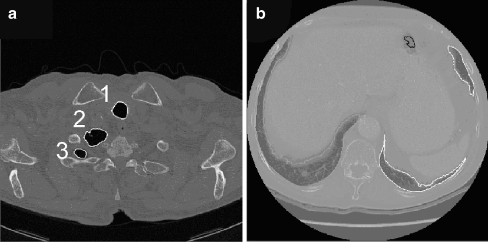
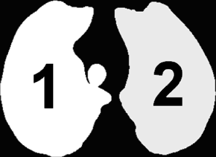
The algorithm is completely three-dimensional. The 3D implementation provides several advantages: it is conceptually simple and effective and it avoids the approximations and incoherences characteristic of 2D techniques. Consider for example Figure 1, where a typical problem of the 2D segmentation algorithm developed in De Nunzio et al.²³ is illustrated. Two slices, taken from the top and bottom parts of the lungs (two different patients) respectively, show incorrect segmentations of the pulmonary parenchyma. In Figure 1a the right lung section, owing to the peculiar shape of the lung top, is split into two disconnected components that may erroneously be classified as belonging to different organs. Figure 1b shows a similar problem in the lower part of the lungs (where the scan also includes the liver and the spleen): the left lung section appears fragmented. In both cases the lung section (obviously connected in 3D) is not 2D connected, so that it may be difficult, for 2D segmentation techniques, to correctly classify each fragment. Figure 2 illustrates what may happen near the hilus, where 2D segmentation algorithms may include (or not) bronchus sections when they are 2D connected (or not) to a lung section. These effects cause coherence faults in adjacent slices, with imprecise segmentation.

Fig. 1.

2D-segmentation inaccuracies from.²³a Top of the thorax: the two lung sections labelled 2 and 3 might be wrongly classified as belonging to different organs, because they are not 2D-connected. b This slice is taken from the low part of the thorax, and shows also the liver and the spleen: the left-lung sections (right part of the image, owing to radiological convention) appear fragmented.

Fig. 2.

2D-segmentation inaccuracies near the hilar region: bronchus sections may be included or not in the segmented areas if they ‘touch’ or do not touch the lung parenchyma (in this figure, a bronchus is touching the right lung, labeled with ‘1’). This leads to incoherence between adjacent slices.

A 3D approach can successfully solve these problems: for example, 3D RG provides a correct segmentation in the cases shown in Figure 1, while the problem exemplified in Figure 2 is solved by removing the extrapulmonary airways with a wavefront simulation model and suitable stop conditions. Also, the accurate removal of the external airway structure by the segmentation process reduces the segmented volume, with the consequent speeding up of the nodule search algorithms, and a reduction of the number of false positives.

Finally, the morphological closing step is implemented in 3D, ensuring coherence between slices.

1. Threshold evaluation

A Hounsfield Unit threshold θ_o, appropriate to discriminate between the lung parenchyma and other tissues, must be defined. For this purpose, the intensity histogram of a set of “central” slices, where the lung sections occupy a large part of the image, is calculated. It is typically bimodal: low-intensity voxels (representing the air and low average density tissues and organs like lungs, bronchi…) and high-intensity ones (belonging to muscles, bones, fat…) fill two large peaks separated by a valley. The threshold value θ_o is set to an approximately central point in this valley, automatically estimated by the isodata algorithm.²⁴

The θ_o threshold is used in step (B) to obtain the reconstruction of the whole respiratory apparatus.

1. 3D Region growing

RG is an iterative technique employed to identify connected regions of interest (contiguous sets of voxels) in images, obeying some inclusion rule (generally based on threshold values), and according to the notion of discrete connectivity. It starts by choosing an initial site (seed point) in the region to be grown and, after checking its neighbors it includes in the growing region only the voxels that meet the inclusion rule. Each included voxel becomes in turn a seed point for the following iteration. The process continues until no voxel is added to the growing area or volume.

In our approach, 3D RG is used to reconstruct the respiratory apparatus. The initial seed point is a voxel belonging to the lung parenchyma, and the inclusion rule selects voxels with intensity values lower than θ_o. In this way the grown connected region is the whole respiratory apparatus, because the growth process fills the lung it starts from, it enters the bronchi and, after crossing the carena, it also fills the opposite lung and the trachea.

The initial seed point is automatically chosen by selecting the central slice of the scan (where the lung sections are large) and picking up the center of the left half of the image; if this voxel does not satisfy the inclusion rule (because it belongs to some dense structures such as a vessel), local random steps are taken looking for a proper point.

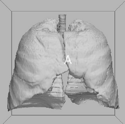
The output of step B (Fig. 3) is a 3D binary mask (M) of the respiratory system, containing both the external airways (trachea and bronchi) and the lungs. All the other low-density regions (the air around the body, esophagus, stomach, or colon if covered by the scan) are not included because they are not connected to the respiratory apparatus.

1. Wavefront simulation for external bronchi extraction

Fig. 3.

3D binary mask of the respiratory system (step B output). It contains both the external airways (trachea and bronchi) and the lungs. The picture (and the following 3D ones) were rendered by the “3d Slicer” visualization and processing software package (www.slicer.org).

The hilus of an organ is a depression or fissure where vessels, nerves, and/or ducts enter the organ itself. In the lungs, this area is superimposed with other structures in a complex way, and it does not have a clear shape or a specific texture, so that its definition and segmentation are difficult and ambiguous.

The segmentation in the hilus pulmonis is an innovative part of this work. We proceed by segmenting the extra-pulmonary airways out, starting from the trachea down to the bronchi entrance into the lungs. After removing the reconstructed sub-tree, the clean-cut lungs remain.

According to Sluimer et al.²⁵ the optimal lung segmentation in the hilus should intersect the bronchial and pulmonary vessel trees at the pleural fold, but the latter is not directly visible in the CT and therefore it cannot be reliably located.

The segmentation of tubular structures, such as the bronchial and vascular trees, is a common subject in literature with many applications in medicine, such as, for example, to measure airway geometry, to study airway reactivity and to guide surgical interventions or in virtual bronchoscopy. Aykac et al.²⁶ describe a fully automatic technique for segmenting the airway tree, by using morphological reconstruction to identify candidate airways on CT slices. Accurate cross-sectional airway measurements are obtained by Tschirren et al.²⁷ by using a method based on fuzzy connectivity, and by Berger et al.²⁸ with a Laplacian of Gaussian filter. Saba et al.²⁹ use a circular cross-section airway model that is adapted to the inner and outer airway walls via a least-square fit. After careful study and, in some cases, test-code writing, none of these methods proved adequate for our application, because our aim was not the complete airway extraction, but rather the segmentation of the external part, starting from the trachea, down to the hilus. As they are formulated, the cited methods give no hint on the hilus position, and therefore do not allow separation of internal from external airways. Moreover, some of them work with a slice per slice approach, instead of being 3D: according to our tests, this methodology severely thwarts investigation on the hilus position.

Wood et al.³⁰ apply a method called “distance tagging”, based on 3D RG, to segment the airway tree of canine lungs. This technique, while filling the airway structure down to the smallest bronchial caliber, creates a map in the growing volume, where the distances of voxels from the seed point are registered. The existence of disconnected groups of voxels with the same distance from the seed suggests the presence of bifurcation points.

Our approach is inspired by Wood’s algorithm, because its progressive, 3D RG nature makes it ideal for obtaining partial airway filling, starting from the trachea. Our aim is the segmentation of only the external part of the bronchi, thus suitable stop conditions are added to stop the growth process at the hilus level; this way the lungs can be accurately isolated from the segmented external airways.

Our multi-pass method combines simple 3D RG (applied to binary mask M and hereafter called M-RG) with a wavefront simulation model; the growth process is appropriately interrupted to avoid flooding into the lung parenchyma.

The suitable initial seed for M-RG is automatically chosen as the centroid of the trachea section in the first of M slices where the trachea appears. To this purpose, the slice ‘objects’ are found (they may be sections from the trachea and possibly from one of the lungs or both) and their maximum vertical coordinate y_max, as measured from the image top downwards, is determined. According to thoracic anatomy, the trachea section is the object with minimum y_max, as we verified in 150 CT scans (the whole 130-image Italung-CT database, with some low-resolution scans added). After locating the trachea, its centroid is calculated and used as a seed.

The M-RG algorithm, unlike ‘traditional’ RG techniques, assigns a label k to each voxel grown at iteration k. The label is therefore equal to the checkerboard distance of the voxel from the starting seed: in this way a distance map is built in the volume. Equally labeled voxels are grouped into connected components (CCs); the set of the CCs with the highest label k (the most recent iteration number) simulates a wave-front, propagating down the airway lumen.

When the wave-front finds a bifurcation (the carena, or bronchi branches) it splits and grows simultaneously down each ramification. Bifurcations are detected by verifying the existence of disconnected components with the same k value.

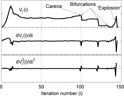
If the M-RG process freely continues until no voxel is added to the growing region, it floods into the pulmonary parenchyma; on the contrary, our aim is to interrupt the process when the wave-front is entering the lungs, ideally while traversing the pleura. Suitable stop conditions must therefore be imposed. For this purpose, CCs in the wave-front are monitored at each iteration (allowing the detection of branches and bifurcation points); the volume (number of voxels) V_j of each (j-th) wave-front CC is studied as a function of the iteration number i. Of course, the number of CCs varies because some are born at branch points, others die when entering blind parts of the airways (due to morphology and to noisy CT data). For a fixed j, V_j(i) is roughly constant when the corresponding CC is traversing tubular (constant transverse-section) ways and the wave-front shape is more or less planar. When a CC enters the lung tissue, it ‘explodes’ filling the volume with spherical (more precisely, parallelepiped-shaped) wave-fronts. So V_j(i) becomes substantially quadratic with i. By imposing suitable test conditions on dV_j(i)/di we identify the wave-front flooding into the lung parenchyma and stop the growth process of component V_j(i). Appropriate conditions must also be imposed on d²V_j(i)/di² to avoid false detections and—after stopping the growth process—backtracking is necessary, because when flooding is detected we are already in the lung, and we have to go back some steps to be more accurate.

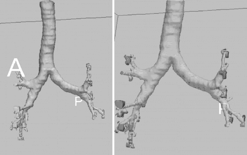
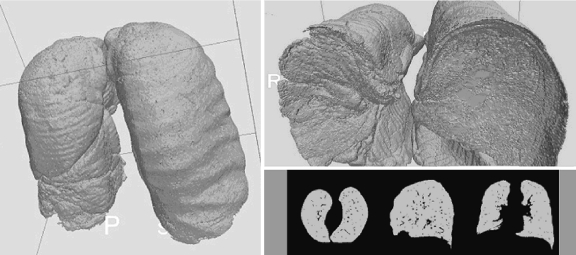
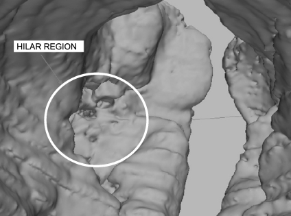
Figure 4 shows a typical V_j(i) and its first and second derivatives; branch points and the flooding into the lung parenchyma are indicated by arrows. In Figure 5 the segmented external airways are shown; after removing them the isolated lungs remain (see mask M′ in Fig. 6) and the hilar region is properly identified (Fig. 7).

1. Solution of the lung “fusion” problem

Fig. 4.

Plot of the volume V_j (with its first and second derivatives) of the wave-front connected components, as a function of the iteration number i in the wave-front propagation process. Branch points (the carena and the following bifurcations) and flooding into the lung parenchyma are evident. Appropriate conditions on the values of V_j(i) derivatives are used to stop the growth process when the wave-front enters the lung parenchyma.

Fig. 5.

The extracted extrapulmonary airways. On the right image, the patches marking the connected components at the boundary with the lung parenchyma are evidenced by means of grey intensities.

Fig. 6.

The lungs, after external airway removal.

Fig. 7.

A detail of the hilar region after trachea and bronchi removal.

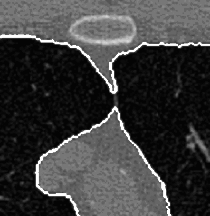
The anterior and posterior junctions between the left and right lungs, in axial CT slices, may be very thin and show a weak contrast. For this reason, and because of partial volume effects, the segmentation algorithms may fail in separating the lungs from each other near these junctions, so that they are erroneously identified as a single object (Fig. 8).

Fig. 8.

Apparent lung fusion: the junction line is so thin and weakly contrasted that the two lung sections appear fused and might be identified as a single structure.

Many solutions to this well-known problem are available in the literature.

In De Nunzio et al.²³ two methods are proposed: a fast one based on 2D morphological operations, and a more precise—but slower—one that makes use of the indentation–detection method, also employed to solve the problem of pleural nodules.¹⁴ Both of those methods had defects: the former was not accurate enough in some cases, because the application of morphological operations led to the production of artifacts; the latter was too slow to be optimal, if compared to the computational cost of the other steps of the algorithm described in this paper.

Brown et al.³¹ use morphologic opening followed by a 2D maximum cost path algorithm; this work inspired Hu et al.,⁹ who follow a dynamic programming approach to find the maximum cost path, corresponding to the junction line position, through a graph with weights proportional to voxel gray-levels. As already said, our experience on the use of morphological operators in the lung-junction region was not completely satisfying, so we decided to explore different strategies not implying the use of morphology.

Shojaii et al.³² apply a watershed transform to locate the lung regions: in their work, lung separation is automatically obtained when a dam is created between the lung catchment basins; their approach is slice per slice and, moreover, no examples of critical lung separation are shown in the paper, so it is difficult to judge about accurateness in case of lung fusion. In Armato et al.³³ the most anterior point along the cardiac aspect of the lung segmentation region is found and a series of rays is used to identify the anterior junction line, which is then turned off. This method is 2D, too.

Our approach to the problem is, at the best of our knowledge, original: it is completely 3D (which was an a priori choice for us, because we wanted to test the advantages of 3D processing over 2D), and is based on the detection of lung fusions and, when they are present, on the construction of a separation surface between the lungs.

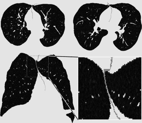
In order to limit the analysis volume, two suitable bounding boxes are defined in M′, in the anterior and posterior junction regions. The part of M′ contained in the boxes is examined to detect a fusion: if it occurs, RG is iteratively performed in the relevant box, each time slightly lowering the threshold used in the inclusion rule, until the lungs get separated from each other (two to four iterations are generally necessary, up to five or six in the worst cases).

When this happens, control points of a separation surface between the lungs are identified. The surface is then calculated by bilinear interpolation and iterative subdivision, until no “hole” is present. The obtained surface smoothly follows the common profile of the two lungs in the contact region: it is used to “turn off” voxels in M′ (the result is mask M″), so that step E (based on RG) will then find the two lungs well separated.

Figure 9 shows an example of separation surface inserted between the lungs, in various axial and coronal projections.

Fig. 9.

The separation surface. Top two axial slices, where separation-surface sections are visible between the lungs. Bottom a coronal projection with a magnified detail.

This step is of great importance to avoiding the introduction of artifacts in the closing stage (step F).

1. Single-lung reconstruction

The reconstruction of the single lungs through two RG applications is now performed on mask M″. To this purpose a seed point is automatically located in each of the lungs, RG is applied and the lung is reconstructed. The two obtained lung masks (M_L and M_R) are passed to step F.

1. Inclusion of pleural and internal nodules, and patching of concavities

M_L and M_R do not enclose dense objects, such as nodules and vessels: they are left out of the grown volume because their density is quite large compared to the lung parenchyma, so they are not included in the growing process. In step F the inclusion of nodules in the segmented lungs is obtained.

Different kinds of lung nodules exist. A number of them are isolated and show good contrast with the surrounding parenchyma. Some are juxta-vascular, i.e., they exhibit a degree of attachment to adjacent blood vessels. A significant fraction is pleural, i.e., contiguous with the pleural surface (we do not distinguish here between nodules originating in the pleura and invading the lung tissue and lung nodules that touch the pleura in their growth process).

While internal (isolated and juxta-vascular) nodules are easy to include in the delimited volume by “filling the holes” in the M_L, M_R masks, pleural ones tend to be considered external to the lungs because of their position and are excluded from the segmented regions.

A variety of algorithmic approaches were suggested to solve the problem. Armato et al. ^34,35 use a 2D ‘rolling ball’ filter applied to the lung segmentation contour to avoid the loss of pleural nodules.

Ko et al.³⁶ calculate the curvature of the lung borders, Gurcan et al.¹⁴ describe an indentation–detection method. Shen et al.³⁷ apply an algorithm for local surface smoothing to the segmented lung contours. A conventional template matching is employed by Lee et al.³⁸ to detect the nodules on the lung wall area, with semicircular models used as reference patterns. Another recent 2D method is based on active contour models and is found in.³⁹

We chose to adopt 3D binary morphologic closing (mask dilation followed by erosion) with a fixed size (30-mm diameter) spherical structural element, to ensure the inclusion of all the types of lung nodules. This size was chosen because this way the operation also encloses the internal vessels in the segmented volume, so that the inclusion of juxta-vascular nodules is guaranteed. According to the scan voxel size (e.g. 0.6 × 0.6 × 1 mm) the structural-element size in voxels is calculated.

By morphologic closing, the mask cavities due to isolated internal nodules and the concavities originated from internal vessels (possibly with juxta-vascular nodules) and pleural nodules are filled. For a formal definition of (con)cavities see.⁴⁰

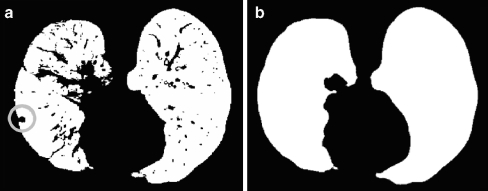
Figure 10 shows how a pleural nodule, initially left out of the segmentation mask by 3D RG, is recovered by the closing step.

Fig. 10.

Comparison between masks M_L ∪ M_R, (a), coming from step E, and M_L^C ∪ M_R^C (b), output from step F, i.e., the lung masks before and after morphological closing. The closing process has included nodules and internal vessels to the mask. As an example, the circle marks a pleural nodule, initially left out of the segmentation mask.

It is now clear why step D, which separates the lung masks into two distinct data matrices, was introduced: the closing operation must be performed on the single-lung masks, because applying it to both lungs at the same time would give undesired results, in particular near the junctions.

The lung masks after the closing procedure M_L^C and M_R^C now cover the pulmonary parenchyma, all the lung nodule types, internal blood vessels, and internal airways.

After this step the lung segmentation process is complete. M_L^C and M_R^C, put together to build up mask M^S, can be applied to the original CT scan to delimit the lung volume. The difference between M^S and M_L ∣ M_R, gives regions of interest where nodules can be searched.

Results and Discussion

As introduced in Methods, the lung segmentation algorithm was initially developed on a set of 130 thorax CT scans from the Italung-CT database. It was later applied to two public databases, one from the ANODE09 competition (55 images) and the other belonging to the LIDC data collection (84 images); the variety of parameters of the tested CT scans allowed us code optimization and error fixing.

The typical algorithm execution time is about 7 min for a 300-slice CT scan, on a two quad-core Intel Xeon CPU workstation (E5345 @ 2.33 GHz, 4 MB cache), equipped with 16 GB RAM. The wave-front step takes about 8 s to segment the extra-pulmonary airways. The lung separation step lasts about 1 min in the worst case. The closing step usually takes about 4 min and still needs optimization. RG operations take 20–30 s per lung.

Qualitative and quantitative tests on the result accuracy were carried on.

Test Against Ground Truth The first test on the results was a check against ground-truth segmentations, performed by our radiologists: the aim of this test was to verify that the automatically obtained segmentation masks accurately followed the lung contours, with correct handling of difficult regions (the hilus, and the top and bottom parts of the lungs).

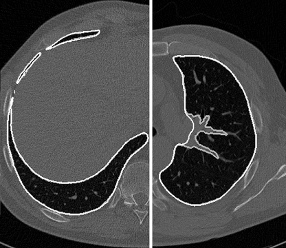
A subset of the CT scans (17 randomly chosen from the Italung-CT database, eight from the ANODE09 set, 11 from the LIDC, giving 36 overall scans) were manually segmented by one of our radiologists and formed the ground truth against which the corresponding automatic segmentations were then checked, slice by slice. Our radiologists considered the automatically and the manually segmented masks in very good agreement. Figure 11 (left) shows an example of correct segmentation in the lower part of the thorax, with the comparison of the manual (gray) and the automatically segmented (white) profiles; the difference between them is hardly noticeable. The same figure, on the right, illustrates a particular situation happening in the central part of the lungs, where the manual and the automatic segmentation purposely do not agree: the vessel entering the lung parenchyma is left out by the manual segmentation (gray), but it is included in the mask by the automatic procedure (white); in this case the difference is a requirement of our algorithm, since leaving vessels out could mean that juxta-vascular nodules might be left out too, which would make this segmentation algorithm inadequate for employing in a CAD system (see also later in this section, “Sensitivity for Nodule Inclusion”, and check for similar situations in Fig. 6 of ³³).

Fig. 11.

Left A correctly segmented lung slice, with the manual and the automatically drawn borders compared. Right A situation where the two borders do not match, because the vessel entering the lung parenchyma is included on purpose (see text) while it is usually left out by manual segmentation.

After qualitative inspection, segmentation metrics were calculated, in order to give more quantitative accuracy measurements. Each manual segmentation was compared to the corresponding automatic segmentation, both by a volume overlap measure, and by a contour distance measure. Statistics were then calculated to evaluate overall accuracy.

Volume Overlap Let T and M be the volumetric binary masks of the ground-truth manual segmentation and of the automatic segmentation procedure respectively (M corresponds to M^S of step F, Methods). Let v be the overlap measure, defined as the ratio of the intersection volume to the union volume (like the well-known Jaccard similarity coefficient):

Here, as usual, symbols “&” and “|” respectively denote the “AND” and “OR” operators between binary matrices. The overlap degree ranges from zero (no overlap) to one (complete overlap). The result of this calculation on the whole dataset gave the average value 0.96 ± 0.02.

Distance Between Automatic and Manual Contours The shape difference between manually and automatically segmented masks was evaluated by first defining the distance between a voxel p_M belonging to the border of mask and the border of mask as follows:

where D_E is the Euclidean distance. Then, for each analyzed CT, the mean, RMS, and maximum distances between the two borders were calculated:

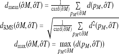Average values on the whole CT dataset were: , , and . They confirm that the automatic segmentations quite correctly reproduce the borders traced by the radiologist.

Since manual segmentation is a slow procedure, not all the images were checked in this way: the remaining ones were divided into two mutually exclusive groups, each separately inspected by one of our radiologists, who visually verified the accurateness of the automatic segmentations.

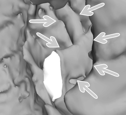
Globally, the test outcome was satisfactory since accurate segmentation was achieved on about 96% of the sample (this percentage is similar in the three tested databases, if considered separately). Figures 5–7, already introduced when illustrating the algorithm, show some successful cases. The remaining 4% of the database images suffered from inaccurate airway tree segmentation, as can be seen in Figure 12; this figure demonstrates what may happen when the airway tree touches the lung surface before the hilar region: because of partial volume effects, the wave-front propagation wrongly leaks into the lung parenchyma at the contact point (as explained in Methods, step C); as a consequence the stop conditions interrupt the segmentation process at a wrong stage. Though this segmentation is not optimal (because some small non-lung structures are included in the segmented volume), it still preserves 3D coherence and smoothness, and most of the airway tree is removed anyway.

Fig. 12.

Inaccurate result. The figure shows what happens when the airway tree touches the lung surface (center of the picture) before the hilar region (seen in the high part); because of partial volume effects, the wavefront floods into the lung parenchyma at a wrong place and the stop conditions intervene: some bronchi (pointed to by arrows), that should be segmented and removed, remain as part of the lungs. The white patch is inserted to accurately visualize the bronchus cut.

Inter-slice Mask Smoothness As already remarked in Methods, 2D segmentation algorithms may suffer from artefacts like those shown in Figures 1 and 2. A test was performed in order to investigate the effectiveness of our 3D approach in terms of inter-slice coherence and smoothness and its advantages with respect to 2D approaches.

In order to assess that our 3D segmentation approach may effectively overcome 2D artefacts, a comparison between the 3D algorithm and our 2D method, derived from the one described in,²³ was performed.

The segmentation masks of the whole CT database were calculated with both the 3D and the 2D algorithms, discarding the images where one of them had severe problems. The segmentation results were quantitatively compared as follows. Let M^2D and M^3D be the volumetric binary-mask outputs of the 2D and 3D segmentation procedures respectively (M^3D corresponds to M^S of step F, Methods). For the sake of simplicity, let M be one of M^2D or M^3D. For each pair of mask slices, indexed by j and k, let s_jk be an inter-slice shape-mask similarity measure, defined as the ratio of the overlap area to the union area of the lung sections in the slices (again, like the Jaccard similarity coefficient):

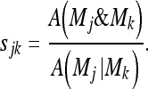Here, M_k is the k-th slice of mask M, A(x) is the area of the objects in x (viz the number of “on” voxels in x) and, as usual, symbols “&” and “|” respectively denote the “AND” and “OR” operators between binary matrices. The degree of “coherence” or smoothness between the pair of adjacent mask sections j, j+1 can be defined as . We shall refer to σ_j as “inter-slice smoothness” or “coherence”.

Since the lung has its own smooth inter-slice profile evolution, the σ_j values are expected to be close to 1; segmentation errors or lack of smoothness would return lower σ_j values.

In order to compare the two segmentation algorithms, and were calculated.

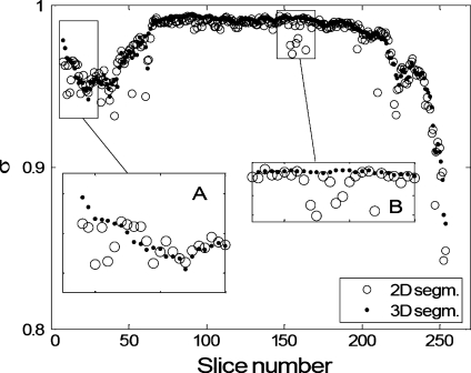
The behaviors of and as a function of j (for the arbitrarily chosen CT scan already represented in Fig. 2) are shown in Figure 13. 2D σ values are almost always lower than the corresponding 3D values. Moreover, is generally smoother than , which shows various outliers that mark the presence of segmentation inaccuracies. Inset A, for example, refers to the lower part of the lungs, where 2D artifacts (coming from the lung morphology shown in Fig. 1b) are frequent. Inset B shows that in the hilar region the 2D segmentation algorithm is probably inaccurate, and in fact these slices include the one in Figure 2; this region was successfully segmented by the proposed 3D approach, while the 2D algorithm success was only partial.

Fig. 13.

Inter-slice smoothness for our 3D algorithm and the 2D segmentation algorithm in,²³ arbitrarily chosen for comparison. Smoothness values are calculated for a randomly chosen CT scan.

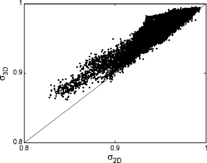
As an example, Figure 14 gives a scatter plot showing and calculated on the whole Italung-CT database.

Fig. 14.

Scatter plot of inter-slice smoothness for our 3D algorithm (σ^3D) and the 2D segmentation algorithm from ²³ (σ^2D), arbitrarily chosen for comparison. Smoothness values are calculated on the whole database described in Methods.

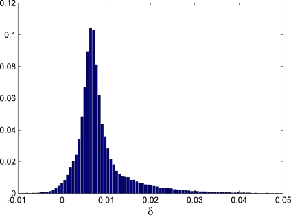
The distributions of and are strongly asymmetric; in the case of the Italung-CT database, for example, their average values are 0.966 and 0.974, respectively, medians are 0.972 and 0.980, standard deviations are 0.017 and 0.019. The average value of the distribution of is 0.008, its median is 0.007 and its standard deviation is 0.006. Being the distribution of δ_j not Gaussian, and asymmetric (its skewness value is 2.1), see Figure 15, in order to test for significance we performed a paired, two-sided sign test (from the Matlab Statistic Toolbox) getting p = 0 within the machine accuracy for the hypothesis that δ_j differences come from a distribution whose median is zero: this shows that Jaccard coefficients are significantly larger than the corresponding , which means that our 3D approach gives better results than the 2D system described in.²³ We get to equivalent conclusions by repeating this procedure for the other two CT databases.

Fig. 15.

Italung-CT database: distribution of (Results and Discussion, Inter-slice mask smoothness).

As a matter of fact, inaccuracies and artifacts in 2D segmentation algorithms can be avoided by the analysis of other slices (at least the ones respectively preceding and following the artifact), which is substantially a 3D operation. Some tests with modified versions of our 2D segmentation software showed that performance of this “partially 3D” approach may be worse than the fully 3D algorithm described in this paper, which a priori avoids these artifacts.

Sensitivity for Nodule Inclusion Since the final goal is nodule searching, the sensitivity of the segmentation algorithm for lung nodule inclusion must be as close as possible to 100%, so that no neoplastic tissue is missed. In order to test the sensitivity, the segmentation masks calculated with our 3D code were automatically checked against the nodule list annotated by radiologists: acting on images containing internal and pleural nodules, the algorithm proved effective in outlining the lung volume without neglecting pathological tissue (100% sensitivity). This test was performed for the Italung-CT images, for the LIDC databases, and for the five annotated cases of ANODE09.

Robustness to Lung Alterations due to Diffuse Lung Disease We could not systematically test our algorithm on lungs containing a variety of diseases yet. The people who participated to the Italung project were asymptomatic smokers; despite the quite large number of nodules found by the radiologists, only a few cases of other diseases were diagnosed. A similar situation was found in the other tested databases, where the focus was on cancer, too. We could anyway apply our software tool to some diffuse interstitial fibrosis alterations (with associated cystic areas) surrounded by a thickened wall, and these images were correctly segmented.

Conclusion

A completely three-dimensional approach to the automated lung segmentation in chest CT scans is proposed. It provides a good basis for a CAD system for lung nodule detection and is being integrated with the Region Growing based nodule search algorithm already developed in¹⁷ within the MAGIC-5 Project.

The algorithm main features are the use of adaptive thresholding, region growing, wave-front simulation, and morphological closing.

Its innovative parts are the treatment of the hilar region, notoriously difficult to be segmented, and the solution of the lung “fusion” problem (caused by partial volume effects).

The algorithm, tested on 269 high-resolution CT scans, provides satisfactory performance, and segmentation quality, showing:

• good accuracy in the lung segmentation, as stated by comparison against ground truth and by visual inspection by our radiologists;

• coherence between adjacent slices;

• 100% sensitivity for nodule inclusion (isolated, pleural, and vascular nodules).

References

- 1.The Lancet, vol. 365, May 14, 2005
- 2.Alberg AJ, Samet JM. Epidemiology of Lung Cancer. Chest. 2003;123:21S–49S. doi: 10.1378/chest.123.1_suppl.21S. [DOI] [PubMed] [Google Scholar]
- 3.Picozzi G, Paci E, Lopez Pegna A, Bartolucci M, Roselli G, Francisci A, Gabrielli S, Masi A, Villari N, Mascalchi M. Screening of lung cancer with low dose spiral CT: results of a three year pilot study and design of the randomised controlled trial ‘Italung-CT’. Radiol Med (Torino) 2005;109(1–2):17–26. [PubMed] [Google Scholar]
- 4.Pastorino U, et al. Early lung-cancer detection with spiral CT and positron emission tomography in heavy smokers: 2-year results. The Lancet. 2003;362:593–597. doi: 10.1016/S0140-6736(03)14188-8. [DOI] [PubMed] [Google Scholar]
- 5.Diederich S, et al. Screening for early lung cancer with low-dose spiral CT: prevalence in 817 asymptomatic smokers. Radiology. 2002;222:773–781. doi: 10.1148/radiol.2223010490. [DOI] [PubMed] [Google Scholar]
- 6.Awai K, Murao K, Ozawa A, Komi M, Hayakawa H, Hori S, Nishimura Y. Pulmonary nodules at chest CT: effect of computer–aided diagnosis on radiologists’ detection performance. Radiology. 2004;230:347–352. doi: 10.1148/radiol.2302030049. [DOI] [PubMed] [Google Scholar]
- 7.Diederich S, Wormanns D, Heindel W, et al. Lung cancer screening with low dose CT. Eur J Radiol. 2003;45:2–7. doi: 10.1016/S0720-048X(02)00302-9. [DOI] [PubMed] [Google Scholar]
- 8.Park M, Wilson LS, Jin JS: Automatic extraction of lung boundaries by a knowledge-based method, visualization 2000, Pan-Sydney Workshop on Visual Information Processing, December, 2000. Conferences in Research and Practice in Information Technology, 2. P. Eades and J. Jin, Eds.
- 9.Hu S, Hoffman EA, Reinhardt JM. Automatic lung segmentation for accurate quantitation of volumetric X-ray CT images. IEEE Trans Med Imaging. 2001;20(6):490–498. doi: 10.1109/42.929615. [DOI] [PubMed] [Google Scholar]
- 10.Brown MS, Goldin JG, Suh RD, McNitt-Gray MF, Sayre JW, Aberle DR. Lung micronodules: automated method for detection at thin-section CT-initial experience. Radiology. 2003;226:256–262. doi: 10.1148/radiol.2261011708. [DOI] [PubMed] [Google Scholar]
- 11.Armato G, III, MacMahon H. Automated lung segmentation and computer aided diagnosis for thoracic CT scans. Int Congr Ser. 2003;1256:977–982. doi: 10.1016/S0531-5131(03)00388-1. [DOI] [Google Scholar]
- 12.Bellotti R, Carlo F, Gargano G, Tangaro S, Cascio D, Catanzariti E, Cerello P, Cheran SC, Delogu P, Mitri I, Fulcheri C, Grosso D, Retico A, Squarcia S, Tommasi E, Golosio B. A CAD system for nodule detection in low-dose lung CTs based on region growing and a new active contour model. Med Phys. 2007;34(12):4901–4910. doi: 10.1118/1.2804720. [DOI] [PubMed] [Google Scholar]
- 13.Chalana V, Sannella M, Haynor DR. General-purpose software tool for serial segmentation of stacked images. Medical Images 2000: Image processing. Proc SPIE. 2000;3979:192–203. doi: 10.1117/12.387675. [DOI] [Google Scholar]
- 14.Gurcan MN, Sahiner B, Petrick N, Chan H-P, Kazerooni EA, Cascade PN, Hadjiiski L. Lung nodule detection on thoracic computed tomography images: preliminary evaluation of a computer-aided diagnosis system. Med Phys. 2002;29(11):2552–2558. doi: 10.1118/1.1515762. [DOI] [PubMed] [Google Scholar]
- 15.Insight-users forum, http://www.itk.org/pipermail/insight-users/2003-September/004762.html
- 16.Bellotti R, Bagnasco S, Bottigli U, Castellano M, Cataldo R, Catanzariti E, Cerello P, Cheran SC, De Carlo F, Delogu P, De Mitri I, De Nunzio G, Fantacci ME, Fauci F, Forni G, Gargano G, Golosio B, Indovina PL, Lauria A, Lopez Torres E, Magro R, Martello D, Masala GL, Massafra R, Oliva P, Palmiero R, Preite Martinez A, Prevete R, Quarta M, Ramello L, Raso G, Retico A, Santoro M, Sitta M, Stumbo S, Tangaro S, Tata A, Zanon E: The MAGIC-5 Project: Medical Applications on a Grid Infrastructure Connection. Proc IEEE Nuclear Science Symposium 16–22/10/2004, Rome, Italy
- 17.Bellotti R, Cerello P, Tangaro S, Bevilacqua V, Castellano M, Mastronardi G, De Carlo F, Bagnasco S, Bottigli U, Cataldo R, Catanzariti E, Cheran SC, Delogu P, De Mitri I, De Nunzio G, Fantacci ME, Fauci F, Gargano G, Golosio B, Indovina PL, Lauria A, Lopez Torres E, Magro R, Masala GL, Massafra R, Oliva P, Preite Martinez A, Quarta M, Raso G, Retico A, Sitta M, Stumbo S, Tata A, Squarcia S, Schenone A, Molinari E, Canesi B: Distributed Medical Images Analysis on a GRID Infrastructure. Future Generation Computer System, Special Issue on Life Science Grids for Biomedicine and Bioinformatics, 23, 2006
- 18.Bottigli U, Cerello P, Cheran S, Delogu P, Fantacci ME, Fauci F, Golosio B, Lauria A, Lopez Torres E, Magro R, Masala GL, Oliva P, Palmiero R, Raso G, Retico A, Stumbo S, Tangaro S: GPCALMA: a tool for mammography with a GRID connected distributed database. Proc. of the Seventh Mexican Symp. on Medical Physics, 682/1:67, 2003, also e-preprint physics/0410084
- 19.Fauci F, Raso G, Magro R, Forni G, Lauria A, Bagnasco S, Cerello P, Cheran SC, Lopez Torres E, Bellotti R, Carlo F, Gargano G, Tangaro S, Mitri I, Nunzio G, Cataldo R. A massive lesion detection algorithm in mammography. Physica Medica. 2005;XXI(1):21–28. doi: 10.1016/S1120-1797(05)80016-X. [DOI] [PubMed] [Google Scholar]
- 20.Cascio D, Fauci F, Magro R, Raso G, Bellotti R, Carlo F, Tangaro S, Nunzio G, Quarta M, Forni G, Lauria A, Fantacci ME, Retico A, Masala GL, Oliva P, Bagnasco S, Cheran SC, Lopez Torres E. Mammogram segmentation by contour searching and mass lesion classification with neural network. IEEE Trans Nucl Sci. 2006;53(5):2827–2833. doi: 10.1109/TNS.2006.878003. [DOI] [Google Scholar]
- 21.Bellotti R, Carlo F, Tangaro S, Gargano G, Maggipinto G, Castellano M, Massafra R, Cascio D, Fauci F, Magro R, Raso G, Lauria A, Forni G, Bagnasco S, Cerello P, Zanon E, Cheran SC, Lopez Torres E, Bottigli U, Masala GL, Oliva P, Retico A, Fantacci ME, Cataldo R, Mitri I, Nunzio G. A completely automated CAD system for mass detection in a large mammographic database. Med Phys. 2006;33(8):3066–3075. doi: 10.1118/1.2214177. [DOI] [PubMed] [Google Scholar]
- 22.Cheran CS, Cataldo R, Cerello P, De Carlo F, Fauci F, Forni G, Golosio B, Lauria A, Lopez Torres E, De Mitri I, Masala G, Raso G, Retico A, Tata A: Detection and classification of microcalcification clusters in digital mammograms. Proc IEEE Trans Med Imaging Conference, 16–22/10/2004, Rome, Italy
- 23.De Nunzio G, on behalf of MAGIC-5 collaboration, “Lung Parenchima Segmentation in CT Scans as a Preprocessing Step for Automatic Nodule Detection", TCN CAE 2005, International Conference on CAE and Computational Technologies for Industry, Lecce (Italy) October 8, 2005
- 24.Ridler TW, Calvard S. Picture thresholding using an iterative selection method. IEEE Trans Systems, Man, and Cybernetics. 1978;8(8):630–632. doi: 10.1109/TSMC.1978.4310039. [DOI] [Google Scholar]
- 25.Sluimer I, Prokop M, Ginneken B. Toward automated segmentation of the pathological lung in CT. IEEE Trans Med Imaging. 2005;24(8):1025–1038. doi: 10.1109/TMI.2005.851757. [DOI] [PubMed] [Google Scholar]
- 26.Aykac D, Hoffman EA, McLennan G, Reinhardt JM. Segmentation and analysis of the human airway tree from three-dimensional X-ray CT images. IEEE Trans Medical Imaging. 2003;22(8):940–950. doi: 10.1109/TMI.2003.815905. [DOI] [PubMed] [Google Scholar]
- 27.Tschirren J, et al. Segmentation and quantitative analysis of intrathoracic airway trees from computed tomography images. The Proceedings of the American Thoracic Society. 2005;2:484–487. doi: 10.1513/pats.200507-078DS. [DOI] [PMC free article] [PubMed] [Google Scholar]
- 28.Berger P, Perot V, Desbarats P, Tunon-de-Lara JM, Marthan R, Laurent F. Airway wall thickness in cigarette smokers: quantitative thin-section CT assessment. Radiology. 2005;235:1055–1064. doi: 10.1148/radiol.2353040121. [DOI] [PubMed] [Google Scholar]
- 29.Saba OI, Hoffman EA, Reinhardt JM. Maximizing quantitative accuracy of lung airway lumen and wall measures obtained from X-ray CT Imaging. J Appl Physiol. 2003;95:1063–1075. doi: 10.1152/japplphysiol.00962.2002. [DOI] [PubMed] [Google Scholar]
- 30.Wood SA, Zerhouni EA, Hoford JD, Hoffman EA, Mitzner W. Measurement of three-dimensional lung tree structures by using computed tomography. J Appl Physiol. 1995;79(5):1687–1697. doi: 10.1152/jappl.1995.79.5.1687. [DOI] [PubMed] [Google Scholar]
- 31.Brown MS, McNitt-Gray MF, Mankovich NJ, Goldin JG, Hiller J, Wilson LS, Aberle DR. Method for segmenting chest CT image data using an anatomical model: preliminary result. IEEE Trans Med Imag. 1997;16(6):828–839. doi: 10.1109/42.650879. [DOI] [PubMed] [Google Scholar]
- 32.Shojaii R, Alirezaie J, Babyn P: Automatic lung segmentation in CT Images using watershed transform. 2005 IEEE International Conference on Image Processing, Genoa (Italy), 2005
- 33.Armato SG, Sensakovic WF. Automated lung segmentation for thoracic CT: impact on computer-aided diagnosis. Acad Radiol. 2004;11:1011–1021. doi: 10.1016/j.acra.2004.06.005. [DOI] [PubMed] [Google Scholar]
- 34.Armato SG, Li F, Giger ML, Doi K, MacMahon H. Computerized lung nodule detection: comparison of performance for low-dose and standard-dose helical CT scans. Proc SPIE. 2001;4322:1449–1454. doi: 10.1117/12.431026. [DOI] [Google Scholar]
- 35.Armato SG, Li F, Giger ML, Doi K, MacMahon H. Automated detection of lung nodules in CT scans: preliminary results. Med Phys. 2001;28:1552–1561. doi: 10.1118/1.1387272. [DOI] [PubMed] [Google Scholar]
- 36.Ko JP, Betke M. Chest CT: automated nodule detection and assessment of change over time—preliminary experience. Radiology. 2001;2002:267–273. doi: 10.1148/radiology.218.1.r01ja39267. [DOI] [PubMed] [Google Scholar]
- 37.Shen H, Goebel B, Odry B: A new algorithm for local surface smoothing with application to chest wall nodule segmentation in lung CT Data, Medical Imaging 2004: Image Processing, edited by J. Michael Fitzpatrick, Milan Sonka, Proceedings of SPIE 5370 (SPIE, Bellingham, WA, 2004)
- 38.Lee Y, Hara T, Fujita H, Itoh S, Ishigaki T. Automated detection of pulmonary nodules in helical CT images based on an improved template-matching technique. IEEE Trans Med Imag. 2001;20:595–604. doi: 10.1109/42.932744. [DOI] [PubMed] [Google Scholar]
- 39.Gargano G, Bellotti R, De Carlo F, Tangaro S, Tommasi E, Castellano M, Cerello P, Cheran SC, Fulcheri C: A novel active contour model algorithm for contour detection in complex objects. Proc. 2007 IEEE International Conference on Computational Intelligence for Measurement Systems and Applications, Ostuni (Italy), 2007
- 40.Aktouf Z, Bertrand G, Perroton L: A 3D hole closing algorithm. In “Lectures Notes in Computer Science”, Vol. 1176. Springer, 1996, pp. 36–47