

Abstract
The goal of data anonymization is to allow the release of scientifically useful data in a form that protects the privacy of its subjects. This requires more than simply removing personal identifiers from the data, because an attacker can still use auxiliary information to infer sensitive individual information. Additional perturbation is necessary to prevent these inferences, and the challenge is to perturb the data in a way that preserves its analytic utility.
No existing anonymization algorithm provides both perfect privacy protection and perfect analytic utility. We make the new observation that anonymization algorithms are not required to operate in the original vector-space basis of the data, and many algorithms can be improved by operating in a judiciously chosen alternate basis. A spectral basis derived from the data’s eigenvectors is one that can provide substantial improvement. We introduce the term spectral anonymization to refer to an algorithm that uses a spectral basis for anonymization, and we give two illustrative examples.
We also propose new measures of privacy protection that are more general and more informative than existing measures, and a principled reference standard with which to define adequate privacy protection.
Keywords: Privacy, computational disclosure control, machine learning
I. Introduction
Data anonymization is the process of conditioning a dataset such that no sensitive information can be learned about any specific individual, yet valid scientific conclusions can nevertheless be drawn. Deidentification, or removing explicit identifiers like names and phone numbers, is necessary but insufficient to protect individual privacy. We must also remove enough additional information so that an attacker cannot infer an identity based on what remains (a reidentification disclosure) or otherwise infer sensitive information about an individual (a prediction disclosure). These kinds of disclosures could be made by examining the data for combinations of variables that might uniquely identify someone, or for patterns of values that unintentionally reveal sensitive information. This is exactly what happened when a reporter reidentified an AOL user in released, deidentified search queries - the combination of several queries was enough to narrow the searcher’s identity to one particular person [2].
The only known way to prevent these disclosures is to remove additional information from the dataset. Most existing methods work by perturbing or suppressing variable values, causing uncertainty in identity inference or sensitive–value estimation. This has been an area of active research for three decades, yet nearly every aspect of it remains an open question: How do we measure privacy protection, and what amount of protection do we want? What is the optimal method of perturbing the data to achieve this protection? How do we measure the impact of the perturbation on scientific analysis, and what is an acceptable impact?
In this paper, we focus on the off-line problem of anonymizing a complete table of microdata, where rows represent records of individuals, and columns represent data variables collected about those individuals. This is in contrast to the more difficult on-line problem of anonymizing each row independently as it is collected or released.
Existing off-line anonymization methods generally fall into the classes of adding noise to the data [3]-[5], swapping cells within columns [6], replacing groups of k records with k copies of a single representative (microaggregation) [7], [8], cell suppression and global variable recoding [9]-[11], and replacing the data with synthetic samples from an inferred distribution [12]-[15]. Some methods involve univariate scale transformation to preserve a selected statistical property [16], [17], but otherwise they all operate in the data’s original space under the original basis. Most operate on one variable at a time, with more advanced methods attempting to take into account some interactions between variables [16], [18].
A common problem with these methods is the difficulty in anonymizing high-dimensional datasets. Since every variable in the dataset can contribute to a pattern that may reidentify a record or reveal sensitive information, the anonymization must involve all variables. Moreover, the more variables there are, the greater each perturbation needs to be to maintain the same level of privacy protection, and the growth is often exponential [3], [16]. This curse of dimensionality has led one researcher to conclude that “when a data set contains a large number of attributes which are open to inference attacks, we are faced with a choice of either completely suppressing most of the data or losing the desired level of anonymity” [19].
The main contribution of this paper is the new observation that the anonymizer is not required to operate in the dataset’s original vector-space basis, and we propose that most if not all anonymization methods could be improved by operating in a transformed basis. This can skirt the curse of dimensionality, simplify the algorithm, or improve the privacy protection or analytic utility of the anonymized data. The second contribution is a set of proposed measures of anonymity that are more generally useful and more informative than previous measures.
The rest of this paper is organized as follows. Section II discusses the new measures we propose to assess the privacy protection of anonymization algorithms, and specifies the existing measures we will use to evaluate analytic utility. Section III describes the generation of a spectral basis for anonymization, its advantages, and our two example applications. Section IV reports the experimental validation of these applications, and Section V discusses the implications and limitations of our approach.
II. Evaluating Anonymization
Anonymization methods must provide both privacy protection and analytic utility. That is, a method must simultaneously prevent the disclosure of sensitive individual information and also allow accurate analysis, usually of statistical trends or associations. How successful an algorithm is depends in part on how these properties are measured. We propose in this section measures of privacy protection that are more generally applicable and more informative than existing measures. We also briefly describe existing measures of basic analytic utility that we will use in our evaluation.
Notation For the rest of this paper we will call the original dataset A and the anonymized dataset . Their columns (variables) will be aj and , and their rows (records) will be Aj or .
A. Disclosure Risk
The threat to privacy from released anonymized data comes from what we will call computational disclosure. Computational disclosure is the breach of confidentiality that occurs when an attacker computationally infers information from a released dataset that the data collectors have pledged to keep confidential. It contrasts with direct disclosure, which is a breach of confidentiality via malicious or accidental release of the original information. Computational disclosure can be divided into two types: reidentification disclosure and predictive disclosure [20], [21].
A reidentification disclosure occurs when an attacker manages to correctly match a particular person’s identity to a particular record in the released anonymized dataset by using auxiliary information. If an attacker can confidently match some combination of attributes from an anonymized record with the same combination from identified auxiliary information, he can transfer the auxiliary identity to the anonymized record. Attempting to make this match is called a matching attack. Its risk is usually assessed under the extremely conservative assumption that the attacker can use the entire original dataset as auxiliary information [22]. Under this assumption, the attack becomes a problem of matching each anonymized record with its corresponding original record. If we can prevent the matching attack from succeeding under these conditions, we can prevent it when the attacker knows far less about the individuals involved.
A predictive disclosure occurs when an attacker manages to predict the approximate, and perhaps partial, content of a target record with the help of the anonymized dataset and some auxiliary information. This risk is interesting because it is not uniquely undertaken by subjects of the data. It is also borne by those in the same underlying population that did not participate in the study, and the data collectors have made no pledge of confidentiality to those non-participants. Furthermore, it is difficult to imagine an application where predictive disclosure is not a desired outcome of the study. In medical applications, for example, the motivation for releasing anonymized data is to allow analysts to draw valid conclusions regarding associations between the data’s variables. We want the anonymized data to preserve associations between smoking and heart attack, for example, or between a particular drug and its side effects. We want physicians to be able to predict disease risk from patients’ symptoms and behavior. This unavoidably allows an attacker to make these same predictions.
So while we appropriately seek to eliminate reidentification risk, we only seek to control the risk of predictive disclosure without eliminating it. While on the one hand, a sufficiently accurate predictive disclosure is really the same thing as a reidentification disclosure, and so it must be controlled, on the other hand a predictive disclosure risk of zero would destroy the analytic utility of the data, so some amount must be allowed. We propose that the proper amount is the predictive disclosure risk that the data presents to non-participants in the study. In other words, the predictive disclosure risk to participants should be no greater than the predictive disclosure risk to non-participants, so that participating in the study does not increase this risk at all.
In previous work, the empirical reidentification rate [22] and k-anonymity [23] have been common risk-assessment measures. These measures turn out to be both unnecessary and insufficient for privacy protection [1]. Moreover, they can only be used in certain constrained situations, and they don’t estimate predictive disclosure risk at all (though some variations on k-anonymity, such as k-ambiguity [24], do attempt to partially reduce predictive disclosure risk). For example, both measures are aimed at preventing an attacker from successfully choosing which original record was the source for a particular anonymized record, and they implicitly assume that this unique original source exists for each anonymized record. With some of our examples, however, an anonymized record has no unique source record, so neither k-anonymity nor the empirical reidentification rate can assess the strength of privacy protection they confer. The k-anonymity measure additionally requires the anonymization to produce groups of k records that are functionally identical, and we will demonstrate that this requirement is unnecessary for strong privacy protection. It is also difficult to make a principled decision of what value for k and what rate of empirical reidentification represents adequate protection.
To overcome these limitations, we propose the new measures prediction distance, prediction ambiguity, and prediction uncertainty to quantify computational disclosure risk. These are more general and more informative than prior measures. Each applies to a single original data point given the whole anonymized dataset. We can calculate the measures for each original point and compare distributions over all points to judge the adequacy of privacy protection. The following paragraphs describe these new measures in detail.
Prediction distance Prediction distance is the distance from a particular original point Aj to the closest anonymized point in , using some distance measure s. It represents the closest an attacker can get to predicting the values of an original data point. To allow scale- and dimensionality-invariant measures, s can be calculated on standardized data and normalized by the number of dimensions m, such as
| (1) |
where xi refers to the ith standardized variable in record x. The prediction distance of an original record Aj would then be
Prediction ambiguity Prediction ambiguity gives the relative distance from the record Aj to the nearest vs. the kth-nearest record in the set . Formally,
where is the ith-closest record in to Aj, under the distance measure s.
An ambiguity of zero means Aj was an exact match to some record in , and an ambiguity of one means that the best match from was a tie among k records. Note that the k tied records are not necessarily identical, but are equidistant from Aj. Intuitively, ambiguity represents the difficulty in selecting the best match from among the k top candidates. Low ambiguity suggests a prominent best match, high ambiguity suggests a crowd of points all equally likely to be the best match.
Prediction uncertainty Prediction uncertainty gives the variation among the k best matches to Aj. Formally,
where is the set of k closest matches to Aj under the distance measure s, and v is a measure of variation, such as the (possibly weighted) average variance of each column in . Intuitively, prediction uncertainty measures the impact of making a poor choice of the best match. If prediction uncertainty is low, then the attacker may be able to predict an accurate value for a sensitive variable even if there are many equally-likely choices for a good match. If uncertainty is high, choosing a good match is much more important.
Between these three measures of prediction risk we can calculate 1) how accurately an attacker can predict the values of an original record, 2) how sure he will be that he has made the best prediction, and 3) the predictive consequences of choosing among the best possibilities. These properties are missed by the empirical reidentification rate and k-anonymity. (Recent variants like k-ambiguity do provide lower-bound goals for prediction uncertainty.)
Mathematically, the new measures are concerned with the local neighborhood of anonymized data points around a given original data point, and how identifiable the original point is among the anonymized crowd. The value for k in the measures reflects the size of the neighborhood considered. In preliminary experiments we found that using large neighborhoods (such as k = 100) for the measures reduced their ability to differentiate between strong and weak anonymization (data not shown). This makes sense, since it is easier to be inconspicuous in a large crowd than in a small one. Smaller neighborhoods, with 5 to 10 neighbors, have worked better for us.
Depending on the application, the three new measures may have unequal importance. For anonymizations with no unique relationship between original and anonymized records, there is no reidentification risk, so prediction distance would be of primary importance. For anonymizations that allow these unique relationships to remain, we may want tighter bounds on ambiguity and uncertainty. We will demonstrate the use of these measures in Section IV. As an interesting point of validation, we note that a recent analysis of matching attacks against a large, public, de-identified (although not anonymized) dataset independently came up with versions of these measures to use in the attacks, based on suitable choices for the distance measure s and variation measure v [25].
Our new measures happily lend themselves to defining a reference standard for what constitutes necessary and sufficient protection against predictive disclosure. Consider a second dataset A* consisting of a sample from the same population as A, but including none of the same individuals. Releasing this nonoverlapping sample A* would clearly pose zero reidentification risk to the subjects of A. It would pose nonzero prediction risk, however, because the records in A* are similar to those in A, and associations learned from one would apply to the other.
We therefore propose using A* as a reference standard for anonymization. If releasing any anonymized dataset imposes a computational disclosure risk to the subjects of A that is no greater than if we had released A* instead, shall be deemed sufficiently protective of its subjects’ privacy. This is a high standard, representing the same protection against computational disclosure as participants would get by opting out of the study. (Of course, other privacy risks remain, such as direct disclosure, but these require preventive measures outside the scope of this work.) Requiring the distributions of our three privacy measures to be no smaller for than for A* provides evidence (but not proof) of meeting this standard.
In some cases, an anonymizer will have the luxury of enough data to set aside a dataset A* for this assessment in addition to the dataset A to be anonymzied. In many cases, however, the anonymizer has no extra data. In these cases a reference standard dataset can be constructed separately for each record Aj by excluding Aj from the original dataset. Taking the distance measure as an example, this means that instead of comparing the distribution of against d(Aj, A*, s) over all records Aj, we compare the distribution of against d(Aj, A–Aj, s), where A–Aj is the original dataset with the record Aj excluded. Achieving a distribution of that is no smaller than d(Aj, A – Aj, s) (and similarly for the other two measures) ensures that according to these measures, releasing the anonymized dataset puts the subjects of A at no greater computational disclosure risk than if they had opted out of the study.
If the subjective assessments of the distributions are unclear on whether the standard is met, a Kolmogorov-Smirnov test can be used with a one-sided null hypothesis that the obtained distribution is equivalent or greater than the reference standard [26], [27]. This would require a statistical definition of ‘equivalent’ that is meaningful in practical terms, such as for example, a vertical difference of 0.05 between the cumulative distributions. Note that contrary to the common use of p-values, in this case a high p-value would be desirable and would indicate sufficient protection.
Given these new measures, we may be tempted to use them as simple anonymization goals. For example, we may consider stating an anonymization goal to achieve a prediction distance of 0.7 for 90% of the data records. This is of course possible, but there are some drawbacks to this approach. First, it is difficult to see how to naturally and defensibly choose such a goal. Second, if the goal is set greater than any portion of the reference distribution, it does represent stronger privacy protection for that portion, but the added protection may come at the expense of reduced analytic utility. And since the reference distribution already represents protection against computational disclosure that is equivalent to nonparticipation, it may be difficult to justify this loss of utility. Therefore, we recommend the anonymization goal of meeting the reference distributions for the new measures, unless there is a clear justification for doing otherwise and the resulting analytic utility is acceptable.
B. Analytic Utility
The most general measure of analytic utility of an anonymized dataset is whether an analyst can draw equally valid conclusions from it compared to the original data [12], [13], [28]. If we know the analyses that the analyst intends to run on the data, we can directly assess the impact by comparing these analyses between the two datasets. Absent this knowledge, we are forced to use a less-than-ideal measurement of analytic impact.
Some algorithms are designed to preserve only specific statistical measures on the data, and therefore can be evaluated in part simply by assessing whether those measures are sufficient for our analytic needs. Detailed comparisons between algorithms that intend to preserve the same measures can be done by assessing how well each algorithm does, in fact, preserve them. The methods we demonstrate here are designed to preserve the univariate means and variances plus bivariate correlations or rank correlations of the data, and possibly some univariate distributions. We will therefore use the preservation of these statistics as measures of analytic utility.
III. Spectral Anonymization
The main contribution of this paper is the observation the anonymizer is not required to operate in the original basis of the dataset, and that by switching to a judiciously chosen alternative basis, we can improve some combination of the privacy protection, the analytic utility, or the computational efficiency of the anonymization. Specifically, we propose that a spectral basis, such as that provided by the data’s eigenvectors, can simplify anonymization methods, improve results, and reduce the curse of dimensionality. We will use the term spectral anonymization to refer to the use of any spectral basis in anonymization. The general approach is to project the data onto a spectral basis, apply an anonymization method, and then project back into the original basis. This section describes the approach in more detail, and gives some simple examples of its use.
Spectral anonymization can usually handle continuous, ordinal, or binary data naturally. Categorical attributes can be accomodated by what is usually known as dummy coding or treatment coding — converting categorical variables with q categories to q binary variables, and recombining them into a single categorical variable after anonymization. Doing this also provides the freedom to treat all discrete variables as continuous for some portion of the anonymization, which can open the way for using some powerful and flexible methods, as we will demonstrate. This does require some extra processing to return the variables to their original discrete state, but we believe the results are worth the extra effort. Since it forms such a fundamental part of our methods, we will discuss this extra processing in a little more detail.
We have found that an initial {−1, +1} binary encoding works best during anonymization, and an inverse logit function works well to transform the (continuous) anonymized values to the [0, 1] range. Our preferred post-processing is to then normalize the q dummy values for each record in the dataset and consider them a probability distribution over the q categories of the original attribute. The first benefit of doing this is that it can be useful to simply release the anonymized data in this state. The record-level probability distribution over the categories acts as a type of local generalization that doesn’t discard nearly as much information as a global generalization or local suppression, but still provides necessary uncertainty about the actual value of the attribute. Depending on the application, this level of privacy and utility may be acceptable.
Nevertheless, other applications may require privacy guarantees that are not met by the probabilistic form, or there may be analyses that require a discrete form for all discrete attributes. In these situations we may convert to a discrete form in several ways. We might, for example, probabilistically sample a single discrete value from these distributions, or we might simply select the discrete value that has the highest probability.
We offer the following concrete example. Suppose we have a categorical variable a with three categories, a ∈ {0, 1, 2} and a data record X with a value for a of X(a) = 2. We first dummy-code the variable for all records, splitting the variable into three dummy variables a0, a1, and a2, and encoding them with ai ∈ {−1, +1}. For the record X, this gives X(a) = X(a0, a1, a2) = (−1, −1, +1). After anonymization, let’s say we have an anonymized record Y (which may or may not have been derived from X) that has values Y(a) = (−2.5, −1.5, +0.41). After the inverse logit transform, we get Y(a) = (0.076, 0.182, 0.601), and after normalization this becomes Y(a) = (0.088, 0.212, 0.700). So the anonymized value for Y(a) is a probability distribution, where Y(a) = 0 with probability 0.088, Y(a) = 1 with probability 0.212, and Y(a) = 2 with probability 0.700. If desired, we can select the discrete value that has the highest probability and release Y(a) = 2, or we can sample from the distribution and release the sampled point - which means 8.8 percent of the time we would release Y(a) = 0, 21.2 percent of the time we would release Y(a) = 1, and 70.0 percent of the time we would release Y(a) = 2.
A. Singular Value Decomposition
Singular Value Decomposition (SVD) [29] provides a useful spectral basis for anonymization. It decomposes a matrix A into A = UDVT, where D is diagonal, and U and V are orthonormal. The columns of U are the eigenvectors of the matrix AAT, the columns of V are the eigenvectors of the matrix ATA, and the diagonal elements of D, also known as the singular values of A, are the squared eigenvalues of both ATA and AAT. The matrices U, D, and V have special properties that can facilitate anonymization.
The first useful property is that the columns of V represent a basis that is optimally aligned (as defined below) with the structure of the data in A. Many datasets have internal structure that keeps them from completely filling the space they reside in, filling instead a potentially smaller-dimensional manifold within the enclosing space. The matrix V represents axes of the space that are rotated to optimally align with the embedded manifold.
The second useful property is that the elements on the diagonal of D give the magnitudes of the data variance or manifold thickness in the directions of this new basis, and the product UD gives the projections of the data onto the basis. Knowing the values of D allows us to make engineering decisions about which axes we wish to emphasize in our anonymization, under the reasonable assumption that the larger dimensions are worth more attention than the smaller ones. The ‘optimality’ of the basis alignment refers to the fact that the first column of V describes the direction with the greatest data variance, and each remaining column gives the perpendicular direction of the greatest remaining variance. This also means that columns of V describe vectors that minimize their average perpendicular distance to the data.
A third useful property of SVD is that the columns of U are uncorrelated. This allows us to anonoymize U one column at a time, skirting the curse of dimensionality, without affecting linear correlations among the variables.
B. Examples
1) Cell Swapping
Simple cell swapping anonymizes a dataset by exchanging the values of selected cells within columns of the dataset [6]. This preserves the univariate distributions of the data but swapping indiscriminately tends to destroy relationships between variables. The challenge is to select cells for swapping that will preserve the statistics of interest. Since choosing swaps that exactly preserve particular statistics is NP-hard [30], swaps are sought that only approximately preserve them.
Approximately preserving even the correlations alone between variables is difficult to do, because it implies several statistical constraints that need to be met [30]. Variations of swapping that attempt to preserve statistical properties have turned out to provide little or no privacy protection [31]-[33], and variations focusing on privacy protection have difficulty preserving multivariate statistics [6]. There is a recent variation that generates synthetic data in a multivariate normal distribution, and then replaces the values in each column with the equally-ranked values from the original data [33]. This variation, called data shuffling, represents the state of the art of cell swapping. It has been shown to provide reasonable privacy protection and to preserve univariate distributions and rank correlations.
Data swapping is well-suited to a spectral variation. Instead of producing the anonymized directly, in spectral swapping we apply a uniform random permutation separately to each column of U (where A = UDVT as above) to produce . We then construct the anonymized by . The permutations of U do not affect the correlations of because the correlation matrix of U is the identity matrix, and our permutations (approximately) preserve this. If we first subtract the column means of A, anonymize, and then replace the means, the spectral variation preserves means, variances, covariances, and linear correlations of the original data. It also preserves the univariate distributions along the principal components of A, which in some cases may be more useful than preserving the univariate distributions of the original variables.
Under anonymization by spectral swapping, the practical reidentification risk is zero because there is no actual unique correspondence between a released record and any individual. As we will demonstrate, the protection that spectral swapping provides against predictive disclosure is stronger than both our reference standard and the comparison data-shuffling algorithm.
A spectral change of basis is therefore sufficient to transform the weak method of simple cell swapping into an algorithm with competitive analytic utility and stronger privacy protection than the state-of-the-art data shuffling algorithm.
2) Microaggregation
Our second example uses the microaggregation method. Microaggregation anonymizes a dataset by collecting similar data points into groups and replacing all k members of the group with k copies of a single representative record. It thus produces a k-anonymous dataset. The representative record may be chosen from the members of the group or it may be derived and calculated from them.
For this example we’ll use the microaggregation method of Recursive Histogram Sanitization (RHS) [5]. RHS is one of the few anonymization methods with rigorously proven anonymity properties, and it demonstrates a large benefit from using a spectral basis. RHS operates by splitting the n-dimensional data at the median in every dimension, forming in one pass a total of 2n potential groups. For a high-dimensional dataset, most of these potential groups will have no members. Of the groups with nonzero membership, if any have membership greater than 2k records, RHS recurses on those groups.
A major problem with RHS that prevents its practical use is that for high-dimensional data, the first pass produces many groups that contain only one member, preventing any anonymization for those records. Our dataset is of sufficiently high dimension to demonstrate this problem.
Spectral-RHS is the spectral counterpart to RHS that works on the T = UD product matrix instead of the original A (Fig. 1). Spectral-RHS makes use of the natural order of singular vectors to prevent the exponential explosion of group formation. In the original RHS, the relative importance of each column of A is unclear, and all columns are necessarily bisected simultaneously. In Spectral-RHS, each successive column of the matrix T spans a smaller range than its predecessor, and we can begin to bisect one at a time based on that ordering. We can continue to select the column with the largest range at any particular step, bisect it at the median, and recurse on the two new groups. Upon the algorithm’s return, the thinner dimensions will probably not have been partitioned at all for most groups, but that makes no difference to the anonymization.
Fig. 1.
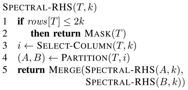
The spectral adaptation of the Recursive Histogram Sanitization procedure. T is the spectral matrix to be anonymized with anonymization parameter k. The procedure Select-Column selects the column of T with the largest range. The procedure Partition(T, i) divides T at the median of its ith column, returning two matrices. The procedure MASK(T) performs the desired masking, such as replacing all elements of T with their mean. The procedure Merge concatenates its array arguments in a vertical stack.
This algorithm illuminates a problem with using the empirical reidentification rate as a measure of anonymity. Since this algorithm replaces a cluster of membership between k and 2k – 1 with copies of a single representative, we expect an empirical matching rate of somewhere between and . However, this non-zero rate does not necessarily mean that the correctly matched records are at higher risk for reidentification. For identities to be at risk, the attacker must be able to distinguish correct from incorrect matches, and the empirical reidentification rate does not expose this distinction. We will show how the new prediction ambiguity distribution does expose it.
IV. Experimental Validation
A. Dataset
A public dataset was obtained from the National Health and Examination Survey (NHANES) [34], with 11763 records of 69 continuous, ordinal, and binary attributes (after converting categorical attributes into binary). The attributes included demographic, clinical, and behavioral variables. Binary attributes were re-coded as {−1, +1}. Categorical attributes were dummy coded with q binary attributes replacing a single categorical attribute with q categories. Anonymized binary attributes were returned to their original representation by using the normalized logit transform of the anonymized results and thresholded at 0.5. Continuous variables were all strictly positive and were log transformed and then standardized. From this we randomly sampled m = 2000 records and selected a representative n = 28 attributes for computational efficiency.
A second sample of 2000 records that did not include any records in the first sample were randomly selected from the same set of 11763 records. This was used as the reference standard in measures of disclosure risk and analytic utility.
B. Anonymization Methods
Spectral swapping and data shuffling [33] were implemented and compared. Spectral-RHS and non-spectral RHS were implemented as described in Section III-B2, both with design parameter k = 5 and the procedure Mask(T) replacing all elements of T with their mean. The choice for k was arbitrary, and typical for microaggregation experiments, and our results are not strongly dependent on it. A smaller value for k generally produces greater utility and weaker privacy protection.
For a baseline comparison, (non-spectral) anonymization by adding zero-mean multivariate normal noise was implemented with a noise covariance matrix bΣ , where b = 0.1 and Σ is the covariance matrix of the original data. The anonymized data was corrected for mean and variance distortion [18], [35]. Noise addition is not an effective method for anonymizing high-dimensional data with many binary attributes, but we include it here as a well-known benchmark.
C. Privacy Protection Measures
Privacy protection was assessed using prediction distance, prediction ambiguity and prediction uncertainty with the distance measure of (1) and k = 5. The value for k was empirically chosen to provide good discrimination between the various anonymization methods.
All assessments were made with the continuous data in the standardized log form described above, original binary data in {−1, +1} encoding, and anonymized binary data in its continuous form. For statistical comparison, the distribution of each measure was compared to the corresponding distribution against the reference sample using the one-sided Kolmogorov-Smirnov test.
For additive noise and Spectral-RHS, reidentification risk was assessed by matching records with the distance measure of (1). The empirical reidentification rate was assessed, and distributions of the three privacy measures were compared between correctly and incorrectly matched records. The area under the receiver operating characteristic curve (AUC) [36] was calculated with the non-parametric empirical method separately for each privacy measure. The AUC measures how accurately each method distinguishes correct from incorrect matches, and is therefore used to indicate whether correct matches are predictably or unpredictably correct.
D. Analytic Utility Measures
Analytic utility was assessed by comparing the differences in the following target statistics between the original and anonymized datasets. The univariate means and variances of each column of the data were calculated, normalized, and compared between datasets, with the median difference over all columns reported. Normalization was done to adjust for differences in scale from column to column. The normalization factor for means was the standard deviation of the column in the original dataset, and the normalization factor for variances was the variance of the column in the original dataset. Additionally, the correlation and rank correlation matrices were calculated, and the (unnormalized) median difference over all entries in each matrix was reported.
E. Results
Privacy Protection The two spectral algorithms improved the privacy protection over their nonspectral counterparts (Fig. 2). Nonspectral RHS failed to produce any anonymization due to the dataset’s high dimensionality - the first pass partitioned all but two records into their own cell, producing distances, ambiguities, and uncertainties of zero. The baseline additive noise algorithm produced some protection, but that protection was much weaker than the reference standard despite the high amount of noise added. Spectral swapping and data shuffling both produced privacy protection superior to the reference standard in all three measures, with spectral swapping providing the stronger protection in each case. Spectral-RHS provided prediction distance better than the reference standard; its uncertainty was zero (weaker than the reference standard) and ambiguity was unity (stronger than the reference standard) by design.
Fig. 2.

Privacy protection of basic spectral anonymization. The distributions of the three anonymity measures over all points in the original dataset are shown as cumuluative probability densities. Curves at or to the right of the Nonoverlapping Sample indicate acceptable protection according to that measure. Spectral algorithms are seen to provide improved privacy protection over their nonspectral counterparts. The measures for nonspectral additive noise are also shown for comparison. Nonspectral RHS failed to anonymize at all, and is not shown.
Under empirical matching, the data anonymized by Spectral-RHS allowed 157 (7.8%) correct matches (Fig. 3). With k = 5, we expected slightly more than this, somewhere between 11% and 20% correct. Correct matches were indistinguishable from incorrect matches on the basis of prediction distance (AUC 0.53), ambiguity (AUC 0.50), or uncertainty (AUC 0.50) (Fig. 3a).
Fig. 3.

Reidentification analysis using the new privacy measures. Correct matches (solid lines) are distinguishable from incorrect (dashed lines) under additive noise anonymization, but not under Spectral-RHS. Reidentification risk is therefore high for additive noise, low for Spectral-RHS. AUC is the area under the Receiver Operating Characteristic curve that results from using the measure as a predictor of a correct match. See Section V for further discussion of these figures.
Additive noise allowed 1984 (99%) correct matches. These were highly distinguishable from incorrect matches on the basis of prediction ambiguity (AUC 0.98) and to a lesser (but still large) extent on the basis of distance (AUC 0.85) or uncertainty (AUC 0.83) (Fig. 3b).
Analytic Utility All methods that produced anonymized data approximately preserved all target statistics, with the exception that Spectral-RHS did not preserve the variance of the original data (Table I).
TABLE I.
Analytic utility measures giving the differences between the statistic in the original data and that in the anonymized data, for the four anonymization methods and the reference standard nonoverlapping sample. A value for an anonymization method roughly equal to or less than that for the nonoverlapping sample indicates sufficient preservation of that statistic. Target statistics are the normalized differences in column means and variances, and differences between entries in the correlation and rank correlation matrix, as explained in the text. All methods are seen to sufficiently preseve all target statistics, except variance was not preserved by Spectral RHS. Nonspectral RHS failed to provide any anonymization at all, so it is not included
| Median difference in | ||||
|---|---|---|---|---|
| mean | var | cor | rank cor | |
| Spectral Swapping | < 10−13 | 0.022 | 0.013 | 0.016 |
| Spectral RHS | < 10−13 | 0.37 | 0.056 | 0.063 |
| Data Shuffling | < 10−13 | < 10−13 | 0.025 | 0.020 |
| Additive Noise | < 10−13 | 0.007 | 0.007 | 0.011 |
| Nonoverlapping Sample | 0.035 | 0.021 | 0.017 | 0.016 |
V. Discussion
The great challenge for an anonymization scheme is to provide adequate privacy protection while minimally affecting the data’s analytic utility. This is difficult to do in general, and is even more difficult to do with high-dimensional data. We have introduced the observation that the anonymizer is not required to operate in the original basis of the data, and that transforming to a judiciously chosen basis can improve some combination of the privacy protection, the analytic utility, and the computational efficiency of the anonymization.
We’ve given two examples of this principle in practice, using the spectral basis provided by SVD. Applications to other methods are not difficult to conceive - additive noise [3]-[5], for example, could be made less disruptive to the multivariate distribution and less susceptible to the stripping attack [37] if the noise were added along the spectral basis vectors instead of directly to the original values. Synthetic methods [12]-[15] could potentially produce simpler or more accurate models in a spectral basis. Cell suppression [9], [23] could be rendered less susceptible to an imputation attack based on correlations, because correlated information would be suppressed as a group, and would therefore be more difficult to replace. Other spectral bases may provide different advantages - exploration of the possiblities is an area for further research.
Additionally, we have proposed new measures for privacy protection and analytic utility that are more general and more informative than existing measures. The measures of prediction distance, prediction ambiguity, and prediction uncertainty quantify how well an attacker can predict the values in a particular original record. They also allow us to gauge the vulnerability of anonymized records to a reidentification attack.
Our experiments demonstrate basic improvements in anonymization that can be made by operating in a spectral basis. In the cell-swapping example, the spectral form of simple swapping provided competitive analytic utility and stronger privacy protection than data shuffling. The practical effect of the stronger privacy protection may be less important, however, since both algorithms give stronger protection than required by the reference standard, and would both therefore be sufficient by that standard. But the example demonstrates that simply choosing a judicious basis for anonymization allows the original, basic cell swapping method to transform from a weak algorithm of mainly historical interest to one that performs as well as the complex state-of-the-art method.
The experiments also demonstrate how spectral anonymization can help overcome the curse of dimensionality. In the microaggregation example, the nonspectral RHS method was unable to anonymize the high-dimensional dataset at all, whereas Spectral-RHS provided sufficient privacy protection as measured by the reference standard.
Additionally, these examples demonstrate some important added value of the new privacy measures. The empirical reidentification rate allowed by the microaggregation example was 8.5%, which would appear unacceptable. But this 8.5% in fact refers roughly to a situation where each original record is approximately equidistant from 12 anonymized records, with an attacker being forced to choose randomly between the 12 in a matching attack. We would expect the attacker to choose correctly about one time in 12, but the attacker is unable to distinguish when that happens.
The distance, ambiguity, and uncertainty curves for Spectral-RHS demonstrate that an attacker could not tell which which empirical matches are correct based on the closeness of the match, since they are nearly identical for correct vs. incorrect empirical matches (Fig. 3a). The AUC value of 0.53 for prediction distance is an objective demonstration that for Spectral-RHS, closer match distance does not at all suggest a correct match (Fig. 3a), and by design of the algorithm neither ambiguity nor uncertainty measurements aid in making that distinction. The privacy protection afforded by Spectral-RHS could therefore be acceptable for many applications — but we wouldn’t know that by looking at the empirical reidentification rate alone.
Our privacy measures tell a different story about anonymization by additive noise. They confirm what we already expected, that this method would be inadequate for our data. Both prediction distance and ambiguity were weaker (lower) under additive noise than for the reference standard, indicating high disclosure risk. Indeed, the empirical reidentification rate was 99%, and correct matches are easily distinguishable from incorrect matches using prediction ambiguity, and to a slightly lesser degree using distance or uncertainty (Fig. 3b). Prediction ambiguity, for example, is much lower for correct matches than for incorrect matches, and would be a reliable indicator of a successful reidentification — one could accept any match with an ambiguity below 0.6, and this would find 90% of the correct matches, with no incorrect matches. We suspect, but did not investigate, that a model built on the combination of the three measures would be even better at predicting correct vs. incorrect matches.
The concept of spectral anonymization is therefore attractive due to its simplicity and power. Intuitively, the benefits of spectral anonymization come from aligning the axes of anonymization to better correspond to the inherent structure in the data. For data with simple structure, the realignment can produce optimal results. Spectral swapping on multivariate normal data, for example, would produce perfect anonymization (in the sense that it meets or exceeds our reference standard) and perfect analytic utility (in the sense that all statistics computed on the anonymized data would be equally valid as those computed on the original data). But this type of data is uncommon in the real world. For real-world data with nonlinear structure, the realignment can help, but further improvements need to be made. The question of how to adapt spectral methods to optimally anonymize data with nonlinear structure is a direction for future research.
ACKNOWLEDGMENT
This work was funded in part by NIH grant R01 LM007273-04A1.
This work was performed while T. Lasko was at the Computer Science and Artificial Intelligence Laboratory of the Massachusetts Institute of Technology, and is based on his doctoral dissertation [1].
Biography

Thomas A. Lasko completed a PhD in Computer Science at the Computer Science and Artificial Intelligence Laboratory of the Massachusetts Institute of Technology, an MD at the University of California, San Diego School of Medicine, and a postdoctoral fellowship at Harvard Medical School. His research interests include medical machine learning and computational disclosure control. He is currently at Google.

Staal A. Vinterbo received his PhD in Computer Science from the Norwegian University of Science and Technology (2000). He is a Research Scientist at the Decision Systems Group, Brigham and Womens Hospital in Boston. He is also an Assistant Professor at Harvard Medical School, and is a member of the affiliated faculty at the Harvard-MIT Division of Health Sciences and Technology. His research interests include machine learning, knowledge discovery and computational disclosure control.
REFERENCES
- [1].Lasko TA. Ph.D. dissertation. Massachusetts Institute of Technology; Cambridge, MA: 2007. Spectral anonymization of data. [Google Scholar]
- [2].Barbaro M, Zeller T, Hansell S. A face is exposed for AOL searcher no. 4417749. New York Times. 2006 Aug. [Online]. Available: http://www.nytimes.com/2006/08/09/technology/09aol.html. [Google Scholar]
- [3].Spruill N. Proceedings of the Section on Survey Research Methods. American Statistical Association; 1983. The confidentiality and analytic usefulness of masked business microdata; pp. 602–607. [Google Scholar]
- [4].Brand R. Inference Control in Statistical Databases. Springer; 2002. Microdata protection through noise addition; pp. 97–116. [Google Scholar]
- [5].Chawla S, Dwork C, McSherry F, Smith A, Wee H. Towards privacy in public databases; Second Theory of Cryptography Conference, TCC 2005; Cambridge, MA. Feb. 2005. [Google Scholar]
- [6].Fienberg SE, McIntyre J. Data swapping: Variations on a theme by dalenius and reiss. Lecture Notes in Computer Science. 2004;3050:14–29. [Google Scholar]
- [7].Torra V, Miyamoto S. Evaluating fuzzy clustering algorithms for microdata protection. Lecture Notes in Computer Science. 2004;3050:175–186. [Google Scholar]
- [8].Domingo-Ferrer J, Torra V. Ordinal, continuous and heterogeneous k-anonymity through microaggregation. Data Mining and Knowledge Discovery. 2005 Sep.11(2):195–212. [Google Scholar]
- [9].Cox LH, McDonald S, Nelson D. Confidentiality issues at the united states bureau of the census. Journal of Official Statistics. 1986;2(2):135–160. [Google Scholar]
- [10].Bethlehem JG, Keller WJ, Pannekoek J. Disclosure control of microdata. Journal of the American Statistical Association. 1990 Mar.85(409):38–45. [Google Scholar]
- [11].Little RJA. Statistical analysis of masked data. Journal of Official Statistics. 1993;9(2):407–426. [Google Scholar]
- [12].Liew CK, Choi UJ, Liew CJ. A data distortion by probability distribution. ACM Transactions on Database Systems. 1985;10(3):395–411. [Google Scholar]
- [13].Rubin DB. Discussion: Statistical disclosure limitation. Journal of Official Statistics. 1993;9(2):461–468. [Google Scholar]
- [14].Dandekar RA, Cohen M, Kirkendall N. Inference Control in Statistical Databases, From Theory to Practice. Springer-Verlag; London, UK: 2002. Sensitive micro data protection using latin hypercube sampling technique; pp. 117–125. [Google Scholar]
- [15].Polettini S. Maximum entropy simulation for microdata protection. Statistics and Computing. 2003;13(4):307–320. [Google Scholar]
- [16].Fuller WA. Masking procedures for microdata disclosure limitation. Journal of Official Statistics. 1993;9(2):383–406. [Google Scholar]
- [17].Clemen RT, Reilly T. Correlations and copulas for decision and risk analysis. Management Science. 1999;45(2):208–224. [Google Scholar]
- [18].Kim J. Proceedings of the Section on Survey Research Methods. American Statistical Association; 1986. A method for limiting disclosure in microdata based on random noise and transformation; pp. 370–374. [Google Scholar]
- [19].Aggarwal CC. On k-anonymity and the curse of dimensionality; VLDB ’05: Proceedings of the 31st International Conference on Very Large Data Bases; 2005.pp. 901–909. [Google Scholar]
- [20].Willenborg L, de Waal T. Elements of Statistical Disclosure Control. 155. Springer; 2001. Predictive disclosure; pp. 42–46. ser. Lecture Notes in Statistics. ch. 2.1. [Google Scholar]
- [21].Willenborg L. Elements of Statistical Disclosure Control. 155. Springer; 2001. Reidentification risk; pp. 46–51. ser. Lecture Notes in Statistics. ch. 2.5. [Google Scholar]
- [22].Winkler WE. Re-identification methods for evaluating the confidentiality of analytically valid microdata. Research in Official Statistics. 1998;1:87–104. [Google Scholar]
- [23].Samarati P, Sweeney L. Protecting privacy when disclosing information: k-anonymity and its enforcement through generalization and suppression; Proceedings of the IEEE Symposium on Research in Security and Privacy; May 1998. [Google Scholar]
- [24].Vinterbo SA. Privacy: A machine learning view. IEEE Transactions on Knowledge and Data Engineering. 2004;16(8):939–948. [Google Scholar]
- [25].Narayanan A, Shmatikov V. Robust de-anonymization of large sparse datasets; IEEE Symposium on Security and Privacy, 2008 (SP 2008); May 2008.pp. 111–125. [Google Scholar]
- [26].Massey FJ., Jr. The Kolmogorov-Smirnov test for goodness of fit. Journal of the American Statistical Association. 1951 Mar.46(253):68–78. [Google Scholar]
- [27].Conover WJ. Practical Nonparametric Statistics. 3rd ed. Wiley; 1999. Tests on two independent samples; pp. 456–465. ch. 6.3. [Google Scholar]
- [28].Fienberg SE, Makov E, Steel R. Disclosure limitation using perturbation and related methods for categorical data. Journal of Official Statistics. 1998;14(4):485–502. [Google Scholar]
- [29].Strang G. Introduction to Linear Algebra. 3rd ed. Wellesley-Cambridge; Wellesley, MA: 2003. [Google Scholar]
- [30].Reiss SP, Post MJ, Dalenius T. Non-reversible privacy transformations; PODS ’82: Proceedings of the 1st ACM SIGACT-SIGMOD Symposium on Principles of Database Systems; ACM Press. 1982.pp. 139–146. [Google Scholar]
- [31].Carlson M, Salabasis M. A data-swapping technique using ranks — a method for disclosure control. Research in Official Statistics. 2002;6(2):35–64. [Google Scholar]
- [32].Moore R. Controlled data swapping techniques for masking public use data sets. U.S. Bureau of the Census, Statistical Research Division; 1996. Report rr96/04. [Google Scholar]
- [33].Muralidhar K, Sarathy R. Data shuffling — a new masking approach for numerical data. Management Science. 2006 May;52(5):658–670. [Google Scholar]
- [34].Centers for Disease Control and Prevention (CDC) National Center for Health Statistics (NCHS) National Health and Examination Survey (NHANES) [Online]. Available: http://www.cdc.gov/nchs/about/major/nhanes/datalink.htm.
- [35].Tendick P, Matloff N. A modified random perturbation method for database security. ACM Transactions on Database Systems. 1994;19(1):47–63. [Google Scholar]
- [36].Lasko TA, Bhagwat JG, Zou KH, Ohno-Machado L. The use of receiver operating characteristic curves in biomedical informatics. Journal of Biomedical Informatics. 2005 Oct.38(5):404–415. doi: 10.1016/j.jbi.2005.02.008. [Online]. Available: http://dx.doi.org/10.1016/j.jbi.2005.02.008. [DOI] [PubMed] [Google Scholar]
- [37].Kargupta H, Datta S, Wang Q, Sivakumar K. Random-data perturbation techniques and privacy-preserving data mining. Knowledge and Information Systems. 2005 May;7(4):387–414. [Google Scholar]