Exploring the factors determining the dynamics of different protein folds

Abstract

Normal mode analyses of homologous proteins at the family and superfamily level show that slow dynamics are similar and are preserved through evolution. This study investigates how the slow dynamics of proteins is affected by variation in the protein architecture and fold. For this purpose, we have used computer-generated protein models based on idealized protein structures with varying folds. These are shown to be protein-like in their behavior, and they are used to investigate the influence of architecture and fold on the slow dynamics. We compared the dynamics of models having different folds but similar architecture and found the architecture to be the dominant factor for the slow dynamics.

Introduction

The function of a protein is tied intimately with the structural modifications it can undergo.¹ Allosteric proteins are obvious examples; their activity is regulated by an effector molecule binding to a site remote from the amino acids primarily responsible for the molecular function (e.g., catalytic site of an enzyme). In this case, the network of interactions between the allosteric and active sites constitutes a dynamical communication pathway within the protein structure. Beyond allosteric regulation, all proteins have dynamical properties that might govern the way their structures respond to their environment (e.g., membrane, substrates, and interacting proteins). The biological role or function of each protein is thus dependent on global dynamical properties, which are encoded in its structure. The dynamical property of a given protein might be seen as its signature or personality¹ and as such is as valuable as information on sequence and structure.

The range of protein motions varies from small and fast, local displacements to slow whole-domain movements.^1–3 Normal mode analysis has been successfully used to investigate the slow motions of protein structures.^4,5 The normal modes of a protein characterize the deformations its structure can undergo and classify them according to their energetic cost. High-energy modes characterize fast, local deformations, whereas low-energy modes correspond to slow deformations with a high degree of collectivity, such as domain movements. Several methods for normal mode analysis have been developed for use with coarse-grained representations of protein structures, and normal mode analysis has become a popular tool for studies of large-scale motions in proteins.^4,6,7

Studies have shown that the slow dynamics are conserved through evolution and that homologous proteins show similar dynamical properties.^8–10 Although the dynamical properties of six nonhomologous proteins sharing a common architecture was analyzed by Keskin et al.,¹¹ most of the studies focus on evolutionary-related proteins at the level of family or superfamily.

In this study, we take a step away from the functional details of families and superfamilies and investigate the dynamical behavior of proteins at the level of fold and architecture. The term “fold” is used to describe the positions of the secondary structures, their type, direction, and connectivity, whereas the term “architecture” refers only to their type and position. The term fold thus corresponds to the topology level in the CATH classification,¹² and architecture corresponds to the architecture level in CATH, but without direction of secondary structure elements (SSEs). We use protein-like computer-generated models.¹³ Built using a modified protein structure prediction pipeline,¹⁴ these models have their architecture and fold defined at the time of construction. A set of possible domain architectures called Ideal Forms¹⁵ is used as a basis for the models, and variation in fold type is generated through connecting the SSEs in all plausible ways.

Using computer-generated models rather than entries from the Protein Data Bank (PDB)¹⁶ allows us to compare the dynamics of protein structures sharing various degrees of structural similarity without being restricted only to experimentally determined structures. The range of structural differences between the models sharing the same fold is in general comparable with what is found within a superfamily. The pipeline yields models where we know the fold by definition, and we can control which folds are present in our dataset. No sequence information is used except to provide secondary structure predictions for the models. Two common αβα-layer folds, corresponding to thioredoxin and flavodoxin-like in the SCOP hierarchy,¹⁷ are used to verify the dynamical behavior of our models.

In this work, we investigate first whether idealized models can be used to recapitulate the dynamical behavior of the fold it represents, and second, we investigate the slow dynamics of fold and architecture. The models we use have clearly defined secondary structures, and it is easy to generate models containing only SSEs. These models provide the basis for determining how much influence the loop connections have on the dynamics. We then compare the dynamics of models with the same architecture but with different folds to see how much difference can be detected.

Results

All models used were generated using the procedure described in the section entitled “Generation of models” from three protein sequences (denoted probe sequences), PDB ids 1f4p, 3chy and 2trx (see Supporting Information). Their structures, extracted from the PDB, are referred to as the native structure and their fold as the original fold. We calculated the normal modes of each model and of the native structures using an elastic network model and a coarse-grained description of the molecules, where each amino acid is represented by a particle located at the position of its C_α atom.¹⁸ Using the normal modes, we computed the associated fluctuation profiles that were used to characterize the deformation patterns of the models and native structures. Note that all particles were treated similarly, and thus, no sequence information was retained in the normal mode calculations (or in the fluctuation profiles). Spearman rank correlation was used to assess the similarity between fluctuation profiles.

Fluctuation profiles of original fold models versus X-ray representatives

We compared the fluctuation profiles of the native proteins to all models that shared the original fold definition. Examples of the fluctuation profiles of each of the three probes can be seen in Figure 1, where the fluctuation values for all residues are plotted sequentially, both for model and corresponding native structure (see “Methods” section for details).

Figure 1.

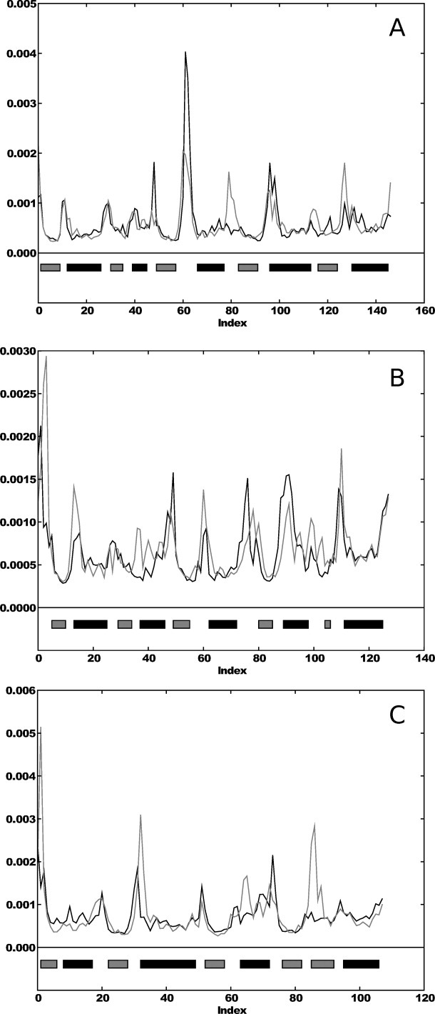
Fluctuation profiles (residue number along X-axis, and fluctuation value along Y-axis) for models and native structures. The fluctuation values of the native structure are indicated in black, and the model values are indicated in gray. (A) The fluctuation profile for a 1f4p model; (B) a 3chy model, both Rossmann fold; and (C) 2trx fluctuation profiles (glutaredoxin). The gray bars indicate β-strands, and the black bars indicates α-helices.

The model fluctuation profiles shown in Figure 1 had the highest correlation to the native structure. A summary of the correlation values of all the models can be found in Table I. The mean correlation for all sets was greater than 0.5. As the models and native structure have the same topology and sequence, all residues (aligned one-to-one) were used to compute the correlation coefficient.

Table I.

Summary Statistics for Rank Correlation Comparison of Fluctuation Profiles Between Native Structure and Models Sharing the Original Fold

Protein	Min	1. quartile	Median	Mean	3. quartile	Max
1f4p	0.104	0.517	0.550	0.536	0.590	0.718
3chy	0.505	0.557	0.576	0.591	0.633	0.667
2trx	0.338	0.510	0.613	0.588	0.670	0.744

Figure 1 shows clearly that the models are similar to their native structures in terms of fluctuation. While the amplitude varies, the shape is similar, and the regions of the structures vary in the same way. The largest fluctuations are found in the loop areas or at the end of SSEs where there is an unrestrained loop.

To verify that this similarity is held for all models and was not due to chance, the fluctuation profiles of the models were compared with a random set of profiles (see “Creating random fluctuation profiles” section) using rank correlation. Figure 2 shows that there is a clear difference in distributions of correlation coefficients when the models were compared with the native structure profiles and with the random profiles.

Figure 2.

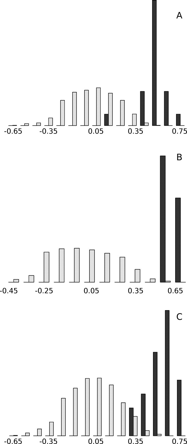
Histogram showing the distributions of correlation coefficients for model profiles compared with the native profiles (black bars) and with the random profiles (light gray bars). (A) 1f4p, (B) 3chy, and (C) 2trx. X-axis shows correlation values, and Y-axis shows proportion of models having a correlation value in a specific interval.

Some of the random profiles obtained aligned the same secondary structures to each other, yielding a somewhat wide distribution of correlation coefficients for the random set. Representing random profiles as simple reversions of the native structure profiles was explored; however, this gives some anticorrelation, as β-strands were aligned to α-helices in the profiles. The distribution of correlation coefficients for comparisons with random profiles is centered around 0, whereas the profiles of the models compared with the native profiles are centered between 0.5 and 0.6. A summary of the random rank correlations can be found in Table II.

Table II.

Summary Statistics for Correlation Coefficients of Fluctuation Profiles Between Random Profile Set and Model Set

Protein	Min	1. quartile	Median	Mean	3. quartile	Max
1f4p	−0.617	−0.157	0.004	0.0002	0.156	0.531
3chy	−0.467	−0.155	−0.003	0.003	0.158	0.574
2trx	−0.605	−0.152	0.0005	−0.0003	0.147	0.528

We also compared the differences between the fluctuation profiles for our comparisons of the models to the native structures, with the differences occurring between natural proteins as described in “Comparing generated models with natural proteins” section. As seen in Figure 3, the differences between the native structures and the models with the same fold definition are comparable with what is found between natural protein domains of the same SCOP superfamily, with the fluctuation of the models being somewhat more robust to structural variation than the SCOP domains. The correlation coefficients obtained for the comparisons shown in Figure 3 were generally lower than those found in Table I because of the differences in the alignments used for comparisons. This was probably due to the model alignments being manually optimized for maximal correspondence between SSEs, a property that cannot be expected to be reproduced perfectly by the DALI algorithm that was used to compute the alignments.

Figure 3.

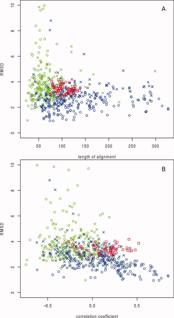
Distribution of structural properties and rank correlation of fluctuation profiles in aligned SCOP domains and generated models aligned to their native counterpart. SCOP domain pairs are colored according to the classification in SCOP common for the two aligned domains: same class only (open green circles); same fold, but different superfamily (green crosses); same superfamily, but different family (blue crosses) and same family (open blue circles). The comparisons with the generated models are shown as red open squares. The correlation coefficient refers to the rank correlation over the aligned parts of the fluctuation profiles. RMSD (Å) is plotted on the Y-axis of both plots, while the alignment length is the X-axis in (A) and correlation coefficient is the X-axis in (B). [Color figure can be viewed in the online issue, which is available at wileyonlinelibrary.com.]

Architecture models versus original fold models

To investigate the impact of loops on the dynamics of the structure, we generated architecture models containing only the secondary structures and not the connecting loops before computing the normal modes used to construct the fluctuation profiles. The profiles of the architecture structures were then compared with the model from which the reduced architecture structure was derived. Figure 4 shows fluctuation profiles similar to those in Figure 1, one plot for each probe protein in the test set. Broken lines in the plot indicate the loop regions that were removed before computing the normal modes of the architecture. Removing the loops resulted in many loose ends in the structure, and as seen from the plots, this is accompanied by increased fluctuations, causing some reduction of the correlation. Table III shows the summary statistics for all correlation coefficients obtained from comparing the fluctuation profiles of the architecture models with their full models. It can be seen that the correlation is very high, averaging more than 0.85, and all the different native structures yielded models with similar flexibilities, even though the folds were different.

Figure 4.

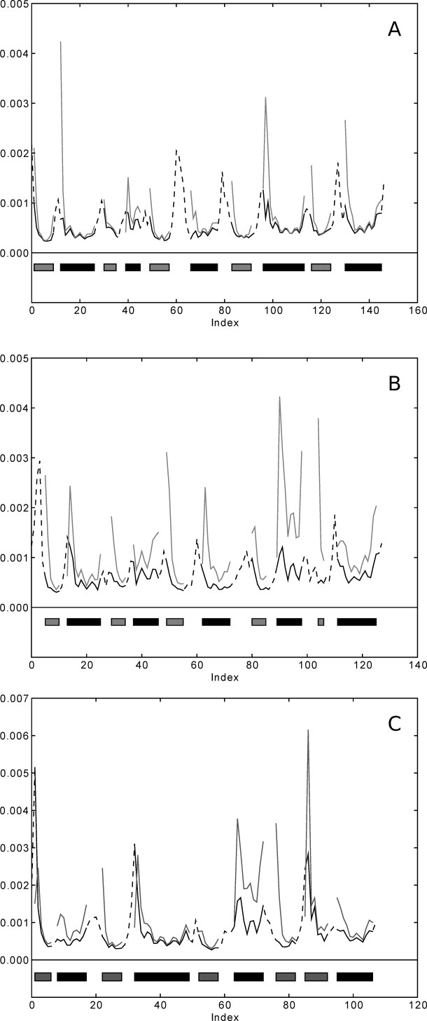
Fluctuation profiles of architecture models (gray lines) and their respective full models (black lines). (A) 1f4p, (B) 3chy and, (C) 2trx. Broken lines indicate gaps in the alignment and follow the secondary structure assignment.

Table III.

Summary Statistics for Rank Correlation Coefficients of Comparison of Fluctuation Profiles for Full Models and Their Architecture Equivalent

Protein	Min	1. quartile	Median	Mean	3. quartile	Max
1f4p	0.790	0.850	0.867	0.872	0.895	0.951
3chy	0.795	0.833	0.844	0.855	0.886	0.913
2trx	0.736	0.839	0.862	0.861	0.883	0.930

Fluctuation profiles of alternative folds versus X-ray representatives

To determine the fold's contribution to the dynamics, we used models based on the same secondary structure content but with different connectivity (Figs. 7 and 8) and computed fluctuation profiles for them. We aligned the profiles as described in “Aligning equivalent parts of different folds” section and computed the rank correlation coefficient between the fluctuation profiles of the models and the corresponding native profile.

Figure 7.

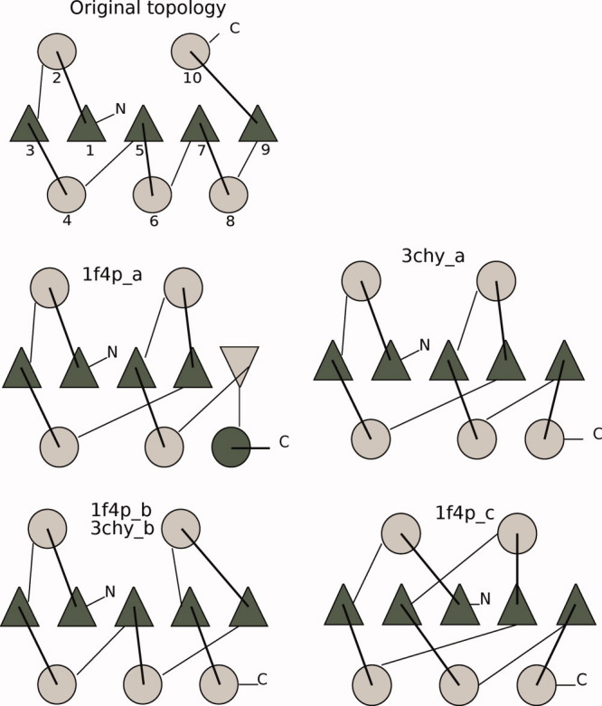
Rossmann fold topology, original, and the four different topologies (two different protein probes). Triangles represent β-strands, and circles represent α-helices. The colors designate the direction of the SSEs, dark gray starting at the back of the page coming at you, and light gray starting in front and traveling back through the page (N-C terminal). The SSEs of the original fold are enumerated in the N-C terminal direction. [Color figure can be viewed in the online issue, which is available at wileyonlinelibrary.com.]

Figure 8.

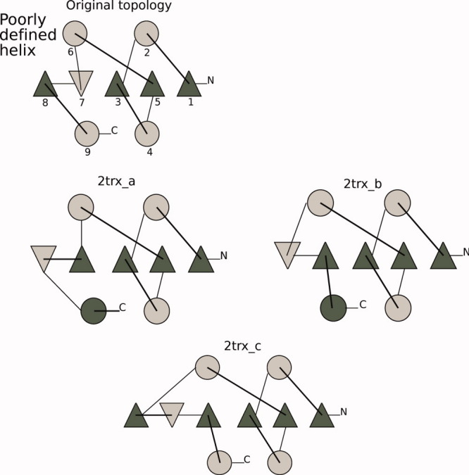
Glutaredoxin fold topologies, both original and three fold variants. The coloring scheme and drawing method matches Figure 7. [Color figure can be viewed in the online issue, which is available at wileyonlinelibrary.com.]

Figure 5 shows the distributions of the correlation coefficients for fluctuation profiles of all model folds, where the equivalent parts of the structures were aligned (both original fold and alternatives). In general, the original fold models had higher correlation coefficients than the alternative fold models.

Figure 5.

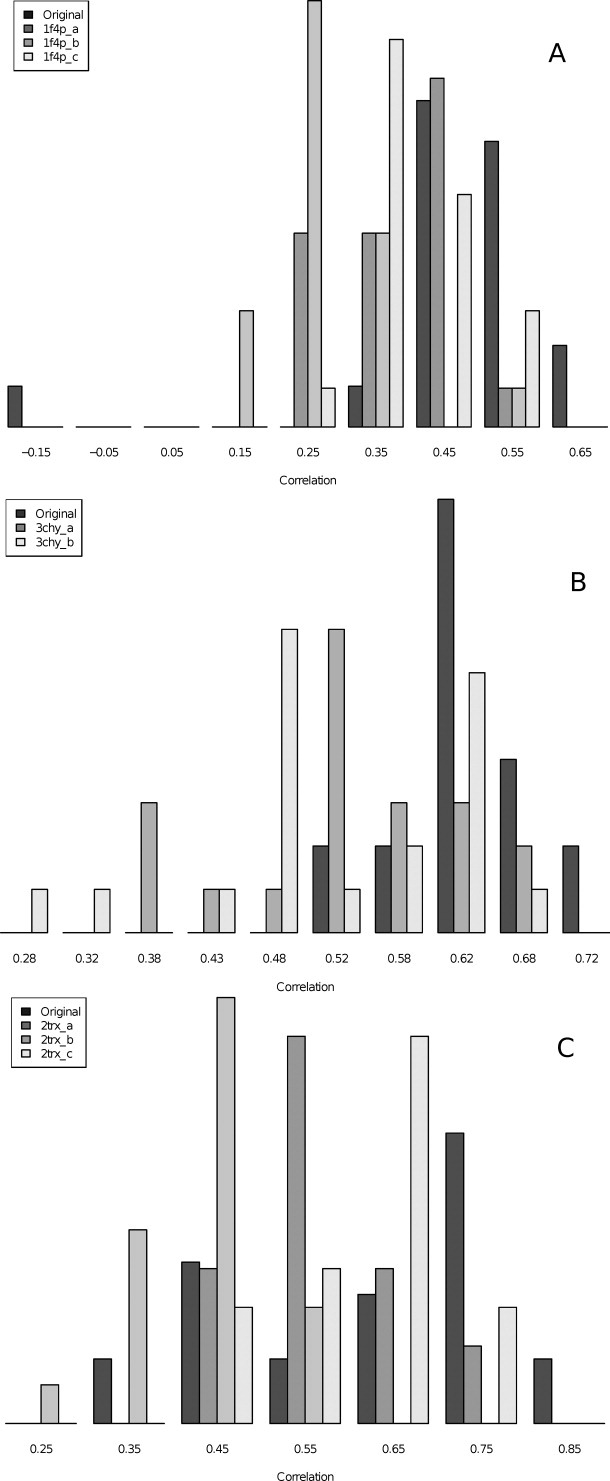
Histograms of the distribution of rank correlation coefficients for comparison between aligned fluctuation values of native (X-ray) profiles and all fold alternatives (also original). Each fold is represented with different shading, the original fold in dark gray. The correlation coefficients are plotted along the X-axis, and the relative number in each group is indicated along the Y-axis.

The distances between the sample distributions of correlation coefficients shown in Figure 5 are shown in Table IV. For each fold, we report the Hodges-Lehmann estimate, which is the median of the differences between all possible pairings of observations from the compared samples. Table IV also shows the P-values from a two-sided Wilcoxon rank sum test for differentiating between the distributions. For the most part, the distributions over the alternative folds exhibited a clear difference for both measures when tested against the original fold. Interestingly, the Hodges-Lehmann estimate for the knotted fold (1f4p_c) was lower than both of the strand swap alternatives (1f4p_a and 1f4p_b), indicating that it is harder to distinguish the original fold from the complex knot than from the strand swaps. Finally, the Hodges-Lehmann estimates for the same fold alternative from the Rossmann fold probes (1f4p_b and 3chy_b) varied.

Table IV.

P-Values from Wilcoxon Rank Sum Tests and Hodges-Lehmann Estimates from Wilcoxon Exact Test for Difference Between Distributions of Rank Correlation Coefficients for Different Folds

Fold 1	Fold 2	P-value	Hodges-Lehmann
1f4p	1f4p_a	0.001235	0.1154503
1f4p	1f4p_b	2.708e−06	0.2208067
1f4p	1f4p_c	0.005211	0.0830413
3chy	3chy_a	0.001116	0.1070684
3chy	3chy_b	0.001349	0.1018550
2trx	2trx_a	0.08757	0.0740576
2trx	2trx_b	2.681e−05	0.2182837
2trx	2trx_c	0.5207	0.03069997

Table V summarizes the correlation coefficient distributions for all probes. The original fold models had a somewhat higher correlation to the fluctuation profiles of the native structures than the fold alternatives had, as indicated by the histograms. We checked the aligned fluctuation profiles against the same type of random background as was done for the models with loops, and the results were comparable with those shown in Figure 2.

Table V.

Summary Statistics for Rank Correlation Coefficients of Comparisons of Fluctuation Profiles Between Native Structures and Models With Different Folds

Fold	Min	1. quartile	Median	Mean	3. quartile	Max
1f4p	−0.119	0.427	0.490	0.468	0.538	0.694
1f4p_a	0.227	0.303	0.391	0.371	0.430	0.574
1f4p_b	0.101	0.216	0.255	0.272	0.347	0.507
1f4p_c	0.280	0.365	0.399	0.409	0.445	0.538
3chy_a	0.361	0.496	0.523	0.529	0.594	0.672
3chy_b	0.297	0.467	0.517	0.522	0.607	0.686
2trx	0.303	0.498	0.672	0.628	0.747	0.808
2trx_a	0.421	0.518	0.573	0.575	0.624	0.711
2trx_b	0.241	0.374	0.454	0.434	0.489	0.565
2trx_c	0.475	0.571	0.629	0.625	0.680	0.761

The top row for each protein shows the data for models with the original fold. The names given to the different folds can be found in Figures 7 and 8.

To get a better understanding of where the differences in fluctuation profiles occurred, we plotted the aligned fluctuation profile of the native probe along with the fluctuation profile for each model (one plot for each fold). Figure 6 shows the fluctuation profiles of all the fold alternatives for the 1f4p probe. As expected, some of the ends of the SSEs were fluctuating more than in the native; however, the trend was generally the same. The plots show the fluctuations of the aligned residues, and all loops are indicated with gray bars. The second helix was poorly defined in the sequence (and in the native structure) and was quite flexible in the models as well, as can be seen from the higher fluctuation values. The fluctuation profiles of a few models diverged from the native, in particular seen in the first few SSEs of the original fold (top left plot), but overall the variability was no more than that would be expected. The fourth helix (SSE 8), which had different loop connections, varied more in the fold alternatives than in the native models, whereas the first part of the structure varied less.

Figure 6.

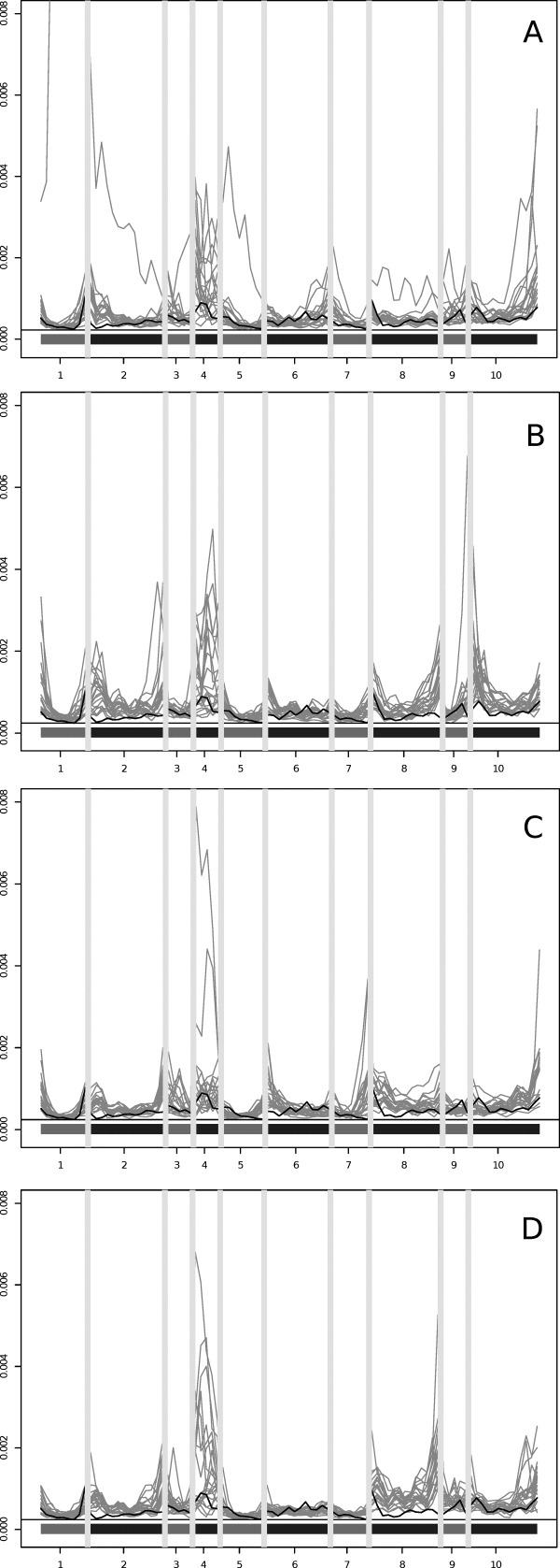
Fluctuation profiles of equivalent residues for the 1f4p probe. (A) The original fold, (B) an inner strand swap, (C) an outer strand swap, and (D) the knotted fold. The gray lines are the model fluctuation profiles, and the thick black line is the profile of the native structure. The gray bars indicate loops. The number along the X-axis corresponds to the SSE numbering in the topmost diagram in Figure 7.

Discussion

We computed the normal modes and fluctuation profiles of three protein structures (1f4p, 3chy, and 2trx) as well as numerous models derived from the same sequences and architectures. Some models shared the original fold while some had alternative folds. We demonstrate that the fluctuation profiles of the models are comparable with those in native structures of the same fold (Table I) and that the similarity is not occurring by chance. Comparisons with values obtained for protein pairs belonging to SCOP families and superfamilies also confirms this.

We see from Figure 3 that the comparison between our models and their corresponding native structures lie in the top range of correlation coefficients obtained for naturally occurring protein domains belonging to the same superfamily, although the structural differences (RMSD) are in a range common for domains of different superfamilies. This may be due to our models being derived from the same sequence (the native protein's sequence) and from a sequence alignment from the same family. The SCOP pairs will also generally align domains with a larger size difference than the comparisons of models with native folds, affecting the average amount and size of gaps in the alignments. All our models have similar secondary structure definitions to the corresponding native structure. In terms of the actual structural diversity present, we represent only a small fraction of what is found in naturally occurring proteins. The similarity in secondary structure definitions mean that although there are differences in the coordinates, the SSEs are well aligned to each other and the occurence of partial alignments of SSEs is unlikely. This means that the variation in fluctuation profiles can be smaller than that for naturally occurring proteins, where the structural variability around the gaps in the alignment can be larger.

As no information specific to residue type is included in the normal mode analysis, we could investigate the contribution of fold regardless of sequence information. This also eased the work of aligning equivalent regions of different folds, and the robustness of structure and dynamics with respect to sequence variation⁸ indicates that this is a reasonable approximation.

Using models where we could control the fold meant that we could choose folds that diverged gradually from the original. Our models represent folds that are close to the original, where one or two SSEs change direction, or where a loop turns into a strand, to more complex changes involving strand swaps and even a knot.

The second aim of this work was to investigate whether the connectivity (fold) or the architecture, that is, the positions of the SSEs, was most important in determining the slow dynamics of a structure. To align different folds, we had to decide which parts of the structure to compare. We settled on comparing the profiles of residues in SSEs in the same position in the architecture. We used only the architecture residues to compute the correlation coefficients; however, the contribution of the loops to the fluctuation profiles was still preserved as all residues were used to compute the normal modes. We decided not to treat SSEs of different orientations in any specific way, and therefore, we aligned the residues from the N- to C-terminal end regardless of which direction the SSEs had in the models. As expected, our calculations showed that changing the direction of the SSEs influences the dynamics as illustrated by the 2trx fold.

The manner in which we chose equivalent residues in different models (and native structures) for comparisons was the same for all models and was based solely on the secondary structure prediction. Although no sequence information was used, the correlation coefficients for the aligned models with original folds were comparable with the same models aligned one-to-one with the native structures (Tables I and V).

We found that the architecture by far dominates fold in determining the slow dynamics. This is rather intuitive when one thinks about the core of the protein with its densely packed structural elements and tight interactions between amino acids. Conversely, the loops are more exposed to the surface, and the interaction network is more sparse. For the same reason, the dynamics of the core is expected to show a higher degree of collectivity than the loops. Keskin et al.¹¹ reached a similar conclusion on the importance of architecture in protein dynamics using an approach slightly different from ours; they used an isotropic network model and X-ray structures of six proteins sharing the same fold (Rossmann fold-like), while we used an anisotropic network model and a larger data set of computer-generated models.

Although architecture is the dominating factor, the loop contribution cannot be overlooked completely as shown from the analysis of the dynamics of the alternative folds. We show that the distributions of Spearman rank correlation coefficients are in general different from those of the original folds (the distributions are not likely to be similar). There does not seem to be a clear relationship between how different two folds are and how different the fluctuation profiles are. The distribution of correlation coefficients from the knotted fold is similar to the distribution of the original fold models. Also, the same alternative fold with a strand swap, 1f4p_b and 3chy_b, has very different distances to their original folds in terms of correlation. The probe sequences are of different lengths, which may impact these results. Another possibility is that one set of models has more interactions due to longer SSEs; however, the difference may also be an indication of the limit of this type of analysis.

The comparison by Spearman rank correlation is stringent in that it treats all regions of the structures similarly; the central positions of the SSEs located in the model cores are treated the same way as residues in loops. Thus, comparisons do not include a bias toward the intuitively most rigid regions.

We believe that the type of computer-generated models we used is a powerful and reliable tool to investigate the dynamics of protein folds. Furthermore, the protocol we developed for fold comparisons may be expanded on and used to address questions about the conservation of dynamics in evolution. Our study shows that while the architecture is dominating in determining fluctuation profiles, the fold cannot be disregarded completely.

Methods

Normal modes calculations

The possible deformations of the native structures and the generated models were characterized by calculating the normal modes of an elastic network representation of the structures. The elastic network representation used¹⁸ represents each residue as a point, located at its C_α-position. The interaction between two such points is described by the pair-potential¹⁹:

(1)

with:

(2)

Here, r_ij is the pair distance vector between the two residues (or points), and R_ij⁰ is the corresponding pair distance vector in the input configuration. The input configuration is defined to be a local minima of the potential. The potential energy of a configuration, R, of the entire elastic network is then taken to be:

(3)

This approximates the residue interactions by a harmonic expression and assumes that the input configuration corresponds to a local minima of the true potential.

The normal modes are the eigenvectors of the matrix K of the second order derivatives of the potential U:

(4)

As we aim to explore the dynamics of architecture and fold independent of the sequence, we express the normal modes in Cartesian coordinates rather than the commonly used mass-weighted alternative. Each normal mode specifies a pattern of deformation as a vector of size 3N, N being the number of residues in the structure. The corresponding eigenvalue is the energetic cost of deforming the elastic network unit length along this mode so that low-energy modes are interpreted as representing the slow, collective motions of the structure and high-energy modes as representing the fast and more local motions of the structure. The six lowest modes have eigenvalues of zero and correspond to rotations and translations of the structure. These are referred to as trivial modes and are ignored in subsequent analyses. The MMTK package²⁰ was used to calculate the normal modes.

The 3N-sized vectors, representing the deformation according to a mode, can be broken down to N displacement vectors of size 3 describing the displacements of each residue in this deformation pattern. The overall fluctuation of each residue can be described as a sum over its displacement in each mode, weighting the lower energy modes favorably relative to the higher energy modes. Specifically, we calculate the fluctuation value for each residue as follows:

(5)

where λ_j is the eigenvalue of mode j, n is the number of modes, and d_ij is the displacement vector for residue i in mode j. This expresses the fluctuations in units of nm² (k_BT)⁻¹, where k_B is the Boltzmann constant and T is the temperature, which is held constant for all our analyses.

The fluctuation values for all residues give a fluctuation profile for a structure. As done in Refs.^9,21,22, we borrow a correlation measure from statistics to quantify the association between two fluctuation profiles. Specifically, we use Spearman rank correlation as this allows us to compare the shape of the profiles rather than the specific values. The rank correlation then represents the degree to which the two profiles behave in the same manner. If the structures are identical, the fluctuation profiles will be identical as well, giving a correlation of 1. If the correlation is around 0, the fluctuation profiles are as similar as would be expected from randomly assigning fluctuations to the residues of the compared structures.

Generation of models

Models were generated using a modified protein structure prediction pipeline,¹⁴ which is summarized here in brief. The overall secondary structure of the models was found by predicting secondary structure from multiple sequence alignments from real proteins and the probe sequence. The secondary structure content dictated plausible architectures.^* A rough C_α model with loop connections was then modeled given the positions of the SSEs on the scaffold. Some folds were not allowed, following rules derived from actual folds found in the PDB. The sequence was then allowed to relax and shift to fit on the structure using a threading method that takes account of the secondary structure prediction and buried hydrophobic side chains.

These rough structures have idealized distances between C_α-positions and SSEs, and the models were then refined using a modeling protocol that relaxed the C_α-coordinates and added backbone atoms before refining the models.

At each step, the models were ranked according to relevant criteria and only the most protein-like models were used.^13,14 At the level of architecture and fold, only architectures resulting in compact, realistic models were chosen. Models with a reasonable solvent exposure and a good match between the predicted secondary structure and burial in the model were retained.¹⁴ Some models were excluded based on unlikely loop connections, for example, loops crossing on the same face or left-handed connections between β-strands. The natural variation of SSEs was taken into account so that all folds were within what occurs naturally.¹³ The sequences were allowed to shift over the template structure, and the models with the best hydrophobic burial were refined from the level of C_α coordinates to full backbone. Finally, the models were refined with respect to bond lengths, bond angles, torsion angles, and other interaction terms.²³

Creating random fluctuation profiles

To demonstrate that our models had meaningful dynamics, we needed a random background distribution to test against. Comparing fluctuation profiles of different structures required that the natural variation of similar structures was represented, as well as a background where there should be no similarity.

As with any characteristic of protein structures, what may constitute random is not well defined.²⁴ The secondary structure content should still be defined, as most structures (and all of our test models) have clearly defined SSEs. The length of the protein must also be similar. Finally, the profiles should be smooth, as the connectivity between residues influences the characteristics, for example, dynamics, of the next residues.

To satisfy these demands, we used the fluctuation profile of the native protein structures as a base to generate a set of random fluctuation profiles. We reversed the profiles and then permuted them by taking the first three fluctuation values and appending them to the end of the list, breaking up the periodicity of the SSEs (both strands and helices). This procedure was repeated for the length of the list (of fluctuation values), giving a large set of semirandom profiles that all had the same overall secondary structure content and interval of fluctuation values as the real structures have, while preserving the length and smoothness of the profiles.

Aligning equivalent parts of different folds

To align different folds to each other, we aligned the SSEs in equivalent positions on the architecture and disregarded the loops. All residues were used to compute the normal modes, but only the fluctuation values in SSEs were used to compute the correlation coefficient between different profiles. The two-dimensional representations of the folds in Figures 7 and 8 show that the architecture of all folds is identical (with the exception of an extra β-strand in one fold). In essence, the SSEs in the same position in the architecture were compared with each other. The secondary structure prediction was used to find the start and end points of each SSE.

The top elements of Figures 7 and 8 show the enumeration of the SSEs in the original folds. Models with the original fold did not require any rearrangements as the order of SSEs of the native structure was used as a basis. For 1f4p_b, which contains a strand swap, the SSEs were rearranged, giving an SSE order of (1, 2, 3, 4, 5, 6, 9, 10, 7, 8). The knotted fold, 1f4p_c, had a larger fold rearrangement. For example, the seventh β-strand (sequentially) is in position one (β-strand number two from the left), while the first β-strand in the sequence is in position five.

For the glutaredoxin fold variants, the fold alignments were easier, as these folds exhibited fewer differences. Only the last parts of the structure were rearranged; however, for consistency, we discounted the loops in these models as well.

Although the fluctuation values of the loops in all models were ignored in the comparisons, the contribution of the loops to the overall structure was taken into account as they are included in the normal mode calculations.

Comparing generated models with natural proteins

To compare results obtained for the generated models with equivalent results obtained for naturally occurring protein domains, a dataset of 760 pairs of such domains was constructed by choosing pairs of varying similarity from the ASTRAL/SCOP40 compendium (release 1.73),²⁵ which offers structural data for a selection of protein domains sharing no more than 40% sequence identity. The pairs were randomly chosen under the constraints that both the different classes and folds of the SCOP hierarchy and the different levels of similarity should be evenly represented. With respect to different levels of similarity, this meant that 25% of the set were classified as the same SCOP family, 25% were classified as the same SCOP superfamily (but as different family), 25% were classified as the same SCOP fold (but as different superfamily), and 25% shared only the SCOP class. All alignments and structural comparisons were performed with DaliLite.^26,27

Dataset

We chose two αβα sandwiches as starting points for this study, the flavodoxin-like Rossmann fold and glutaredoxin, a thioredoxin fold. These are similar in architecture, but the folds are quite dissimilar (see the topmost elements of Figs. 7 and 8). The Rossmann folds, PDB codes 1f4p (147 residues) and 3chy (128 residues), and one glutaredoxin fold, PDB code 2trx (108 residues), were used as probes to generate models. The sequence was used only to get a secondary structure prediction (in a multiple alignment with other members of the same sequence family). The number of residues, secondary structure prediction, and architecture were then used to generate models for each protein. We generated models that had the same fold as the probe proteins (original fold), and some with a different fold. Figures 7 and 8 show both the original and the alternative folds for the Rossmann fold probes and the glutaredoxin probe, respectively. The number of models for each fold varied somewhat from 10 (Rossmann fold based on the 3chy probe) to a little more than 20.

The ensemble of models sharing the same fold should be comparable with a superfamily or fold in the SCOP classification.¹⁷ Measuring on a residue-to-residue basis gives RMSD values of between 3 and 6 Å for models with the original fold superposed on the native probe structure. The similarity between the models was around 3–4 Å on average, although some models were more similar and had an RMSD value of as low as 1 Å.

We are interested in how the large-scale motions change between folds, and therefore, we chose models with varying levels of fold differences. We included examples of strand swaps for all starting probes, both in the middle of the sheet and at the edge. Some folds also had SSEs that were reversed in direction. Finally, one glutaredoxin alternative had an extra strand and one of the Rossmann fold probes was knotted, giving altogether seven alternative folds. One alternative fold was represented by both Rossmann fold probes.

References

- 1.Henzler-Wildman K, Kern D. Dynamic personalities of proteins. Nature. 2007;450:964–972. doi: 10.1038/nature06522. [DOI] [PubMed] [Google Scholar]
- 2.Reuter N, Hinsen K, Lacapere JJ. Normal mode analysis of the Ca2+-ATPase based on a comparison between the E1Ca and E2TG Structures. Biophys J. 2003;84:2186–2197. doi: 10.1016/s0006-3495(03)74644-x. [DOI] [PMC free article] [PubMed] [Google Scholar]
- 3.Zheng W, Brooks BR, Thirumalai D. Allosteric transitions in the chaperonin GroEL are captured by a dominant normal mode that is most robust to sequence variations. Biophys J. 2007;93:2289–2299. doi: 10.1529/biophysj.107.105270. [DOI] [PMC free article] [PubMed] [Google Scholar]
- 4.Ma J. Usefulness and limitations of normal mode analysis in modeling dynamics of biomolecular complexes. Structure. 2005;13:373–380. doi: 10.1016/j.str.2005.02.002. [DOI] [PubMed] [Google Scholar]
- 5.Skjaerven L, Hollup SM, Reuter N. Normal mode analysis for proteins. Theochem. 2008;898:42–48. [Google Scholar]
- 6.Bahar I, Rader AJ. Coarse-grained normal mode analysis in structural biology. Curr Opin Struc Biol. 2005;15:1–7. doi: 10.1016/j.sbi.2005.08.007. [DOI] [PMC free article] [PubMed] [Google Scholar]
- 7.Rueda M, Chacon P, Orozco M. Thorough validation of protein normal mode analysis: a comparative study with essential dynamics. Structure. 2007;15:565–575. doi: 10.1016/j.str.2007.03.013. [DOI] [PubMed] [Google Scholar]
- 8.Maguid S, Fernandez-Alberti S, Parisi G, Echave J. Evolutionary conservation of protein backbone flexibility. J Mol Evol. 2006;63:448–457. doi: 10.1007/s00239-005-0209-x. [DOI] [PubMed] [Google Scholar]
- 9.Maguid S, Fernandez-Alberti S, Echave J. Evolutionary conservation of protein vibrational dynamics. Gene. 2008;422:7–13. doi: 10.1016/j.gene.2008.06.002. [DOI] [PubMed] [Google Scholar]
- 10.Maguid S, Fernandez-Alberti S, Ferrelli L, Echave J. Exploring the common dynamics of homologous proteins. Application to the globin family. Biophys J. 2005;89:3–13. doi: 10.1529/biophysj.104.053041. [DOI] [PMC free article] [PubMed] [Google Scholar]
- 11.Keskin O, Jernigan RL, Bahar I. Proteins with similar architecture exhibit similar large-scale dynamic behavior. Biophys J. 2000;78:2093–2106. doi: 10.1016/S0006-3495(00)76756-7. [DOI] [PMC free article] [PubMed] [Google Scholar]
- 12.Orengo CA, Michie AD, Jones S, Jones DT, Swindells MB, Thornton JM. CATH—a hierarchic classification of protein domain structures. Structure. 1997;5:1093–1108. doi: 10.1016/s0969-2126(97)00260-8. [DOI] [PubMed] [Google Scholar]
- 13.Taylor WR, Chelliah V, Hollup SM, MacDonald JT, Jonassen I. Probing the ‘dark matter’ of protein fold space. Structure. 2009;17:1244–1252. doi: 10.1016/j.str.2009.07.012. [DOI] [PubMed] [Google Scholar]
- 14.Taylor WR, Bartlett GJ, Chelliah V, Klose D, Lin K, Sheldon T, Jonassen I. Prediction of protein structure from ideal forms. Proteins: Struct Funct Bioinformatics. 2008;70:1610–1619. doi: 10.1002/prot.21913. [DOI] [PubMed] [Google Scholar]
- 15.Taylor WR. A Periodic Table for protein structure. Nature. 2002;416:657–660. doi: 10.1038/416657a. [DOI] [PubMed] [Google Scholar]
- 16.Berman HM, Westbrook J, Feng Z, Gilliland G, Bhat TN, Weissig H, Shindyalov IN, Bourne PE. The protein data bank. Nucleic Acids Res. 2000;28:235–242. doi: 10.1093/nar/28.1.235. [DOI] [PMC free article] [PubMed] [Google Scholar]
- 17.Murzin AG, Brenner SE, Hubbard T, Chothia C. SCOP: a structural classification of proteins database for the investigation of sequences and structures. J Mol Biol. 1995;247:536–540. doi: 10.1006/jmbi.1995.0159. [DOI] [PubMed] [Google Scholar]
- 18.Hinsen K. Analysis of domain motions by approximate normal mode calculations. Proteins. 1998;33:417–429. doi: 10.1002/(sici)1097-0134(19981115)33:3<417::aid-prot10>3.0.co;2-8. [DOI] [PubMed] [Google Scholar]
- 19.Hinsen K, Petrescu AJ, Dellerue S, Bellissent-Funel MC, Kneller GR. Harmonicity in slow protein dynamics. Chem Phys. 2000;261:25–37. [Google Scholar]
- 20.Hinsen K. The molecular modeling toolkit: a new approach to molecular simulations. J Comput Chem. 2000;21:79–85. [Google Scholar]
- 21.Halle B. Flexibility and packing in proteins. Proc Natl Acad Sci USA. 2002;99:1274–1279. doi: 10.1073/pnas.032522499. [DOI] [PMC free article] [PubMed] [Google Scholar]
- 22.Micheletti C, Carloni P, Maritan A. Accurate and efficient description of protein vibrational dynamics: comparing molecular dynamics and gaussian models. Proteins: Struct Funct Bioinformatics. 2004;55:635–645. doi: 10.1002/prot.20049. [DOI] [PubMed] [Google Scholar]
- 23.MacDonald JT, Maksimiak K, Sadowski MI, Taylor WR. De novo backbone scaffolds for protein design. Proteins: Struct Funct Genet. 2010;78:1311–1325. doi: 10.1002/prot.22651. [DOI] [PMC free article] [PubMed] [Google Scholar]
- 24.Taylor WR. Decoy models for protein structure score normalisation. J Mol Biol. 2006;357:676–699. doi: 10.1016/j.jmb.2005.12.084. [DOI] [PubMed] [Google Scholar]
- 25.Brenner SE, Koehl P, Levitt M. The astral compendium for sequence and structure analysis. Nucleic Acids Res. 2000;28:254–256. doi: 10.1093/nar/28.1.254. [DOI] [PMC free article] [PubMed] [Google Scholar]
- 26.Holm L, Park J. DaliLite workbench for protein structure comparison. Bioinformatics. 2000;16:566–567. doi: 10.1093/bioinformatics/16.6.566. [DOI] [PubMed] [Google Scholar]
- 27.Labarga A, Valentin F, Anderson M, Lopez R. Web services at the European Bioinformatics Institute. Nucleic Acids Res. 2007;35:W6–W11. doi: 10.1093/nar/gkm291. [DOI] [PMC free article] [PubMed] [Google Scholar]