Multiplexed Wavelet Transform Technique for Detection of Microcalcification in Digitized Mammograms

Abstract

Wavelet transform (WT) is a potential tool for the detection of microcalcifications, an early sign of breast cancer. This article describes the implementation and evaluates the performance of two novel WT-based schemes for the automatic detection of clustered microcalcifications in digitized mammograms. Employing a one-dimensional WT technique that utilizes the pseudo-periodicity property of image sequences, the proposed algorithms achieve high detection efficiency and low processing memory requirements. The detection is achieved from the parent–child relationship between the zero-crossings [Marr-Hildreth (M-H) detector] /local extrema (Canny detector) of the WT coefficients at different levels of decomposition. The detected pixels are weighted before the inverse transform is computed, and they are segmented by simple global gray level thresholding. Both detectors produce 95% detection sensitivity, even though there are more false positives for the M-H detector. The M-H detector preserves the shape information and provides better detection sensitivity for mammograms containing widely distributed calcifications.

TODAY, BREAST CANCER is the most frequent form of cancer in women and also the leading cause of mortality.¹ There is clear evidence that early diagnosis and treatment significantly increase the chance of survival.^2,3 Among the different diagnostic methods available for detection of breast cancer, mammography is widely recognized as the chief modality for early detection in asymptomatic women.³

One of the early symptoms of breast cancer is the appearance of microcalcification clusters, which have a higher X-ray attenuation than the normal breast tissue and appear as a group of small, localized, granular bright spots in mammograms. Popular methods for computer-aided detection of clustered microcalcifications include the difference image,⁴ multiscale processing based on fuzzy pyramidal linking,⁵ and spatial filtering techniques.⁶ An efficient method for the detection of microcalcification must be capable of detecting objects with very small but varying sizes. Recently discovered multiorientation and multiresolution properties of the human visual system⁷ has led to the idea of wavelet-based multiresolution analysis for detection of microcalcification.

A wavelet transform (WT) is a decomposition of an image onto a family of functions called a wavelet family. Contrary to the conventional transforms having a fixed resolution in the spatial and frequency domain, the resolution of a WT varies with a scale parameter, decomposing an image into a set of frequency bands. This variation in resolution helps the WT to characterize the irregularities in an image locally. The wavelet approach has been used for contrast enhancement, detection, and segmentation^{8, 9, 10} of microcalcifications.

In this article, we represent the microcalcification detection as an edge detection problem. A one-dimensional (1-D) processing technique based on a discrete wavelet transform (DWT) is employed for detection. The image sequences are found to be pseudoperiodic when treated as 1-D signals. Taking the multiplexed wavelet transform (MWT), ie, DWT over samples that are spaced one period apart,¹¹ leads to a representation of these pseudoperiodic signals in terms of regularized oscillatory components plus period-to-period fluctuations. Hence the edge information gets pushed into the detail spaces more efficiently than is the case with conventional DWT. The edge detection methods using 2-D operators smear the edge information as a smoothing operation always precedes the edge detection operator. But smoothing is very important, because the differential operators are very sensitive to noise.^12,13 Because the method proposed here uses a 1-D processing technique, the gray level transitions of an edge in the orthogonal direction will not be disturbed.¹⁴ Moreover, the processing memory requirement is reduced to a size equal to the length/breadth of an image from that of the whole image in the 2-D DWT methods.

MATERIALS AND METHODS

Detection of Microcalcification as an Edge Detection Operation

Microcalcifications, small concentrations of calcium in the breast, represent an early sign of possible cancerous growth. Individual calcifications are not worrisome; but when they appear in groups, they can indicate a potential tumor. Five or more calcifications, measuring less than one millimeter, in a volume of one cubic centimeter, define a “cluster.” The probability of malignancy increases as the size of the individual calcification decreases and also when the total number of calcifications per limit area increases. The risk increases when they are heterogeneous in size and shape. The major constraint in their detection is the low contrast between normal and malignant tissues, especially in younger women. Their small size also contributes to a lower subject contrast. The assumptions made with regard to the nature of the microcalcifications are as follows:

1. They are of higher frequency than the surrounding breast tissue, hence they appear brighter.

2. They are usually 0.1 to 1 mm in size.

3. The average calcification is roughly circular, and can be treated as a circular-symmetric Gaussian function.

Discrete Wavelet Transform

Wavelets are basis functions in a vector space comprising a scaling function φ with its associated wavelet function ψ and their dual functions

and

. The basis functions at scale j, and translation or shift k in the case of 1-D may be denoted by {φ_j,k} and {ψ_j,k}, j,k∈Z, where

1

The dual functions are defined in a similar way.

For fast DWT computation a sub band filtering scheme is used, where φ and ψ are represented by the corresponding discrete filters g(n) and h(n), n∈Z, respectively, called the decomposition or analysis filters. Furthermore, there exist the reconstruction or synthesis filters as the dual filters

(n) and

(n). The wavelet and scaling transform coefficients X_j and β_j of a signal x(n) at any level j are given by

2

where, j = 1,2...J; n, k∈Z, β₀[n] = x[n], the input signal. The synthesis equation is:

3

where γ_J[n] = β_J[n] and γ₀[n] = y[n], the reconstructed signal, which is the same as the input signal x[n].

To apply wavelet decomposition to images, 2D extension of wavelets is required. This can be achieved by the use of separable or non-separable wavelets. In this article, we consider separable wavelets only. From the 1D basis, it is possible to construct a 2-D separable wavelet basis with four basis functions, one sealing function

(x, y), and three wavelet functions

(x, y), τ ∈ {1,2,3} given by:

4

These basis functions span the four j-level linear vector spaces rather than just two as in the 1-D case. An analogous definition holds for the dual scaling function

(x, y) and the wavelet function

(x, y).

2-D Discrete Wavelet Transform

The M-level wavelet representation of a 2-D function f is given by

5

The approximation and the detail coefficients in the above expression are

and

respectively, where <.,.> denotes the inner product in the l² (Z²) space. The 2-D basis given by equation (4) may be represented by the four possible tensor products gg, gh, hg, and hh of the 1-D filters g and h. Let c^j and d^j,τ− denote the 2-D sequences

and

, k,l ∈ Z and τ = {1,2,3}. The scaling and wavelet transform coefficients at a coarser level, j+1, are computed from c^j by convolution followed by downsampling, as follows:

6

for j = 0,1,...,M−1. Here * denotes 2-D convolution and (↓↓2) denotes downsampling by a factor of 2 in both the x and the y directions. The given image is treated as c⁰.

To perform the 2-D DWT computation as above, instead of using the 2-D filters, one can employ a separable extension of the 1-D decomposition algorithm. The rows of the data are convolved with the first 1-D filter and every other column is retained. The above process is repeated column-wise using the other 1-D filter. Further stages of 2-D decomposition are obtained by recursively applying the procedure to the low-pass filtered output of the previous stage.

The wavelet reconstruction is performed recursively, starting at level M by upsampling (denoted by ↑↑2) followed by convolution using the dual filters. The signal reconstructed at the jth-level from coefficients at the j + 1th level may be expressed as:

7

Edge Detection Using Wavelet Transform

Recently, a new edge filter based on WT was proposed by Mallat and Zhong.¹⁵ They combined the properties of WT and a gradient method to form a “multiscale” edge detector. In their work, the first derivative of a cubic spline function is utilized to detect the local extreme values of WT as edge points. However, the ultimate goal of the work was to efficiently compress the input image. Therefore, although the adopted wavelet is capable of detecting edges, the performance of edge detection was not a major concern in their work.

Most multiscale edge detectors smooth the signal at various scales and detect sharp variation points from their first or second derivatives. The extrema of the first derivative corresponds to the zero-crossings of the second derivative and to the inflation points of the smoothed signal. It is proved that if a wavelet is the second derivative of a smoothing function, the zero crossings of the WT indicate the location of the sharper signal variations.¹⁵

Any function θ(x) whose integral is equal to 1 and that converges to 0 at infinity can be considered as a smoothing function. An example is a Gaussian function. Let θ(x) be a function twice differential and let

By definition, ψ^a (x) and ψ^b (x) can be considered to be wavelets because their integral is equal to zero. The WT of a function f(x) at scale s and position x computed with respect to ψ^a (x) and ψ^b (x) is defined by:

8

9

The local extrema of

thus correspond to the zero crossings of

and to the inflation points of f * θ_s (x). In the particular case, θ(x) is a Gaussian, the zero-crossing detection is equivalent to a Marr-Hildreth edge detection,¹⁶ and extrema detection corresponds to a Canny edge detection.¹⁷

This can easily be extended to the 2-D case. Here, we have to use a 2-D smoothing function θ (x, y), whose integral over x and y is equal to zero and converges to 1 at infinity. Edges are defined as points (x₀, y₀) where the modulus of the gradient vector is the maximum in the direction towards which the gradient vector points in the image plane f * θ_s (x, y). Relating this to a 2-D WT, one can locate the edge points from the two components

f (x, y) and

f (x, y), as discussed in the 1-D case.

Multiplexed Wavelet Transform

The concept of MWT was first proposed by Evangelista¹¹ as a class of transforms for the representation of pseudo-periodic signals with constant period. This transform simplifies the analysis of the pseudo-periodic signals by decomposing them into a regular asymptotically periodic signal and a number of fluctuations over this signal.

The MWT of a signal x(n), of period M, is defined as the set of coefficients

10

where j = 1,2...; k is an integer; q = 0,1,2...M−1. ζ_j,k,q (n), the multiplexed wavelets, are defined as

11

given a complete and orthonormal set of ordinary wavelets ψ_j,k (n).

The Inverse MWT (IMWT) is given by

12

In this work, images are treated as oscillatory signals, although they are not periodic in a strict mathematical sense. The periods along the horizontal and vertical directions are taken to be the width and the length of the image segment, respectively. Any pixel in an image of size L × W can be represented as V_q(r) or V_r(q) where r = 1,2...L−1 and q = 1,2...W−1. Considering its periodicity along the vertical direction alone, the J-level MWT of the image may be expressed as

13

where j = 1,2...J; k ∈ Z and φ_j,k, the scaling function associated with the wavelet function ψ_j,k.

are the MWT coefficients of the signal V_q(r) at jth scale and kth shift, and

are the multiplexed scaling transform coefficients of the same section of the signal at Jth scale and kth shift (residue after J levels of MWT decomposition). Similar expressions are obtained by considering the image as a 1D signal along the horizontal direction as well.

From Eq (13) we can see that in the MWT, the WT is taken over samples that are spaced one period apart. Hence, the interperiod fluctuations of the signal are better sieved out in the wavelet partials, whereas the residue holds the asymptotically periodic information. It is quite different for the DWT, where the oscillatory part, as well as the fluctuations, gets filtered into different wavelet and scaling partials altogether, depending on the frequency content of the signal. A comparison between MWT and 2-D DWT techniques on a simple synthetic image using “Bior 6.8,” a biorthogonal wavelet basis, is shown in Figure 1. Figure 1b and c are, respectively, the images reconstructed from the third-level MWT and DWT scaling partials of the original image shown in Figure 1a.. The illustrations clearly show that the edge information gets precisely filtered into the wavelet partials of the MWT, leaving its scaling partials with only the edges blurred, whereas additional information is lost from the scaling partials of DWT. Hence, accurate reconstruction of the edges can be achieved from the MWT wavelet partials.

Figure 1.

Comparison of performance of discrete wavelet transform (DWT) and multiplexed wavelet transform (MWT) for edge detection. (a) Original image; (b) image reconstructed from third-level MWT scaling partials; (c) image reconstructed from third-level DWT scaling partials.

PROPOSED METHOD

This section describes the novel WT-based 1-D processing techniques for detecting and segmenting microcalcifications in digitized mammograms. The edge features formed by microcalcifications located in parenchymal structures are detected using the zero-crossings/local extrema of the MWT coefficients. The use of zero-crossings results in a M-H edge detector and the local extrema results in a Canny edge detector.¹⁸ We have selected the Biorthogonal wavelet “bior 1.3” of support 6 for edge detection. The level of processing required depends on the resolution of image data. It has been experimentally determined that a 3-level decomposition is sufficient for detecting the microcalcifications from the images in the databases we have used.

The interperiod fluctuations corresponding to the intensity changes along the horizontal direction are determined by computing the MWT of the image up to the desired level, taking it to be periodic along the vertical direction. Similarly, considering the periodicity along the other direction, the MWT is computed to give the edge information along the vertical direction. Singular points are determined from the zero-crossings /local extrema of the MWT coefficients along both directions. The isolated single-pixel intensity changes, ie, noise, are eliminated by retaining only those zero-crossings that hold a parent–child relationship¹⁹ between the coarsest level and the finest level of detail. In this way the sensitivity of the differential operators to noise is taken care of without smearing the edges.

The retained points are boosted appropriately to enhance the edge features. The IMWT is applied to these points to get the horizontal and vertical edge maps, which are then combined and scaled to get the complete microcalcification information. Global gray-level thresholding based on image statistics is applied to the combined edge map to segment possible microcalcifications. The threshold T is selected to be proportional to the mean of the reconstructed edge map “M” i.e., T = kM; k has been experimentally determined to be a real number such that 1 < k < 2. Because we are adopting a 1-D processing technique, a single row/column is considered for processing at a time. The implementation consists of the following steps:

• Step I: MWT computation. Computation of the MWT coefficients up to the desired level for a row/column of the image.

• Step II: Removal of noise. Discarding all zero-crossings/ local extrema that do not hold a parent–child relationship between finer to coarser levels.

• Step III: Inverse transform. Scalar multiplication of the retained coefficients to boost them and take the inverse transform. Steps I to III produce the edge map for a single row/column. These steps are repeated for all rows/columns to get the complete horizontal/vertical edge maps.

• Step IV: Thresholding. Global gray-level thresholding is used on the combined edge map to segment possible microcalcifications.

Detection Criteria

The results are expressed in terms of sensitivity or “true positive” (TP) and specificity or “false positive” (FP). As there are no universally accepted detection criteria, we have selected the criteria proposed by Karssemeijer.⁶ Accordingly, for counting TPs, a cluster is considered detected if two or more microcalcifications are found in the region of film identified by an expert radiologist. A FP is counted if two or more erroneous detections are made within an empty closed region of 0.5 cm width.

Data

We have tested the algorithm on an ensemble of 40 mammograms (22 mammograms altogether containing 27 microcalcification clusters, 3 with distributed calcifications, and 15 normal ones) taken from the freely distributed digitized mammograms of the Mammographic Image Analysis Society (MIAS) database of the University of Essex, England.²⁰ The images in the database are digitized at 50-micron pixel edge, which are then reduced to 200-micron pixel edge and clipped or padded so that every image has 1024 × 1024 pixels. The accompanying “Ground Truth” contains details regarding the character of the background tissue, class, severity, and coordinates of the center of the abnormality and approximate radius of the circle enclosing it.

We have also validated the algorithms using a local database consisting of 40 mammograms, containing 28 microcalcification clusters in 27 mammograms and 13 normal studies. The mammograms in the local database were collected from restricted mammographic centers and scanned using a UMAX Powerlook III scanner at a resolution of 2000 pixels/square inch. The abnormal regions in these mammograms were identified by an expert radiologist.

RESULTS AND DISCUSSION

Typical examples of microcalcification detection using the two methods are illustrated for three mammograms in Figure 2. The images clearly indicate that the shape of the cluster is preserved in the M-H method compared to Canny method. This is due to the symmetric nature and the ability of the M-H operator to form closed contous. The M-H edge detector provides better detection sensitivity for mammograms containing widely distributed calcifications.

Figure 2.

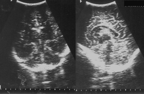
Comparison of detection of microcalcifications from various mammograms using Canny and Marr-Hildreth (M-H) detectors. (a) Sections of original mammograms containing a well-defined microcalcification cluster: (left) hard to find cluster (middle) widely distributed calcifications (right); (b & c) microcalcifications detected by Canny and M-H detectors, respectively, from the mammograms in (a).

The detection capability of the two proposed methods and the conventional 2D DWT method are tabulated in Table 1 for different thresholds. The number of TPs, FPs, and missed TPs (MTP) for two different values of k are shown for the MIAS database, as well as the local database. It can be seen that as the threshold is increased the FPs decrease, but the sensitivity is also decreased. For screening mammography applications, where a high rate of FP is not tolerable, a high threshold is preferred. In diagnostic applications, sensitivity is the important factor and hence smaller thresholds are to be used.

Table 1.

Comparison of Sensitivity and Specificity of Microcalcification Detection Using Canny, Marr-Hildreth (M-H), and Conventional 2D Discrete Wavelet Transform (DWT) Detectors for Two Values of k Such That k₁ > k₂.

MIAS Database
k	Canny			M-H			2D DWT
	MTP	TP	FP	MTP	TP	FP	MTP	TP	FP
k1	2	25	22	2	25	24	6	21	31
k2	15	12	9	14	13	9	18	9	12
Local Database
k1	2	26	20	2	26	22	4	24	29
k2	12	16	8	10	18	10	15	13	6

MTP: missed true positive; TP: true positive; FP: false positive; MIAS: Mammographic Image Analysis Society (Essex, UK).

The application of our algorithm on the MIAS database resulted in a TP identification rate of 95%, against 0.6 FP clusters per image for the M-H edge detector (Table 1). (Rate of FP is computed considering all 40 images). With the locally obtained mammograms, a TP identification rate of 93% at the rate of 0.55 FP clusters per image was obtained. The Canny method produced the same TP detection rate at the cost of a slightly lower FP per image, 0.55 for the MIAS database and 0.5 for the local database.

Detection can be achieved using any of the biorthogonal wavelets. We have selected “bior1.3,” one of the smaller biorthogonal wavelets. It is found that the shape of the cluster is captured more accurately by the larger biorthogonal wavelets such as “bior4.4,” “bior 5.5,” and “bior6.8.” This is probably because these filters approximate the response of the human visual system, in the sense that they are similar in form to the Laplacian of Gaussian described by Marr.¹⁶

To further validate our algorithm, we have compared it with some of the state-of-the art algorithms that have used the same database. By applying a triple ring filter to the MIAS database, Ibrahim et al.²¹ claim to have obtained a sensitivity of 95.8% with a FP rate of 1.8 clusters/image. They have used 43 mamograms, 24 normal ones and 19 others, each containing one microcalcification cluster. Vilarrasa et al.²² have used morphological operations to remove noise background and came up with a TP rate of 85% on the MIAS data set. By multiscale morphological operations and entropy thresholding, Melloul and Joskowicz have arrived at a TP rate of 93.75%.²³

CONCLUSIONS

Microcalcification detection using two wavelet-based edge detectors was performed and the performance of the two detectors was evaluated. We were able to achieve 95% detection accuracy for the MIAS database. It has been found that the M-H edge detector retains the shape information of the clusters, which is essential for classification. Also, it detects distributed microcalcifications more efficiently. Both methods are suitable for detecting subtle microcalcifications that could not be detected by other methods. Because the 1-D processing technique employed here will not smear the edge information in the orthogonal direction, better detection efficiency is obtained. Moreover, the processing memory requirement is reduced to the size of one row or column, from that of the whole image for a 2-D operator.

References

- 1.Kopans DB. Breast Imaging, Philadelphia: J. B. Lippincott Company; 1989. [Google Scholar]
- 2.Lester RG. The contribution of radiology to the diagnosis, management, and cure of breast cancer. Radiology. 1984;151:158. doi: 10.1148/radiology.151.1.6701296. [DOI] [PubMed] [Google Scholar]
- 3.Smith RA. Epidemiology of breast cancer categorical course in physics, Technical Aspects Breast Imaging. Radiol Soc North Am. 1993;.:21–33. [Google Scholar]
- 4.Chan HP, Doi K, Vyborny CJ, et al. Improvement in radiologist’s detection of clustered microcalcifications on mammograms: the potential of computer aided diagnosis. Invest Radiol. 1990;25:1102–1110. doi: 10.1097/00004424-199010000-00006. [DOI] [PubMed] [Google Scholar]
- 5.Lo BC, Chan HP, Lin JS, et al. Artificial convolution neural network for medical image pattern recognitions. Neural Netw. 1995;8:1201–1214. doi: 10.1016/0893-6080(95)00061-5. [DOI] [Google Scholar]
- 6.Karssemeijer N. A stochastic method for automated detection of microcalcification in digital mammograms. Information Prooess Digit Imaging. 1991;76:227–238. [Google Scholar]
- 7.Wiesel TN. Post natal development of the visual cortex and the influence of environment. Nature. 1982;229(5883):583–591. doi: 10.1038/299583a0. [DOI] [PubMed] [Google Scholar]
- 8.Qian W, Chian W, Clarke LP, et al. Tree structured non-linear filter and wavelet transform for microcalcification segmentation in mammography In: Acharya RS, Goldgof DB, et al., editors. : Biomedical Image Processing and Biomedical Visualization. Proc: SPIE; 1993. pp. 509–520. [Google Scholar]
- 9.Strickland RN, Hann HI. Wavelet transforms for detecting microcalcifications in mammograms. IEEE Trans Med Imaging. 1996;15:218–228. doi: 10.1109/42.491423. [DOI] [PubMed] [Google Scholar]
- 10.Yoshida Y, Doi K, Nishikawa RM, et al. Automated detection of clustered microcalcifications in digital mammograms using wavelet processing techniques. Medical Imaging, Proc. SPIE. 1994;2167:868–886. [Google Scholar]
- 11.Evangelista G. Comb and multiplexed wavelet transforms and their applications to signal processing. IEEE Trans. Signal Process. 1994;42:292–303. doi: 10.1109/78.275603. [DOI] [Google Scholar]
- 12.Gonzales RC, Wintz P. Digital Image Processing. Reading, MA: Addison-Wesley; 1987. [Google Scholar]
- 13.Shirai Y. Three Dimensional Computer Vision. New York: Springer-Verlag; 1985. [Google Scholar]
- 14.Kiran KP, Sukhendu D, and Yegnanarayana B: One dimensional processing for edge detection using Hilbert transform. In Proceedings of the Indian Conference on Computer Vision, Graphics and Image Processing (ICVGIP 2000), 25–31, 2000
- 15.Mallat S, Zhong S: Characterization of Signals from Multiscale Edges. IEEE Trans. Pattern Analysis and Machine Intelligence 14:710–732, 1989
- 16.Marr D. Vision. San Francisco: W.H. Freeman; 1982. [Google Scholar]
- 17.Canny J. A computational approach to edge detection. IEEE Trans. Pattern Analysis and Machine Intelligence, 1986;PAMI-8:679–698. doi: 10.1109/TPAMI.1986.4767851. [DOI] [PubMed] [Google Scholar]
- 18.Mini MG, Devassia VP, Thomas T. Detection of microcalcification in digitized mammograms using wavelet transform local extrema. J Digit Imaging. 2003;16(Suppl. 1):8–10. doi: 10.1007/s10278-004-1020-8. [DOI] [PMC free article] [PubMed] [Google Scholar]
- 19.Shapiro JM. Embedded image coding using zero trees of wavelet coefficients. IEEE Trans. Signal Process. 1993;41:3445–3462. doi: 10.1109/78.258085. [DOI] [Google Scholar]
- 20.Suckling J, et al. The Mammographic Image Analysis Society Digital Mammogram Database. Exerpta Medica. International Congress Series. 1994;1069:375–378. [Google Scholar]
- 21.Ibrahim N, Fujita H, Haray T, et al. Automated detection of clustered microcalcifications on mammograms: CAD system application to MIAS database. Phys Med Biol. 1997;42:2577–2589. doi: 10.1088/0031-9155/42/12/021. [DOI] [PubMed] [Google Scholar]
- 22.Vilarrasa A, Gimenez V, Manrique D, et al.: A new algorithm for computerized detection of microcalcifications in digital mammograms. Proceedings of the Int. Conference on Computer-Aided Radiology and Surgery, CARS’98:224–229, 1998
- 23.Melloul M, Joskowicz L: Segmentation of microcalcification in x-ray mammograms using entropy thresholding. Proceedings of the International Conference on Computer-Aided Radiology and Surgery, CARS, 2002