Compartmentalization increases food-web persistence

Abstract

It has recently been noted that empirical food webs are significantly compartmentalized; that is, subsets of species exist that interact more frequently among themselves than with other species in the community. Although the dynamic implications of compartmentalization have been debated for at least four decades, a general answer has remained elusive. Here, we unambiguously demonstrate that compartmentalization acts to increase the persistence of multitrophic food webs. We then identify the mechanisms behind this result. Compartments in food webs act directly to buffer the propagation of extinctions throughout the community and augment the long-term persistence of its constituent species. This contribution to persistence is greater the more complex the food web, which helps to reconcile the simultaneous complexity and stability of natural communities.

For decades, ecologists have sought to understand what leads to stable and persistent ecosystems (1–7). Recently, it was demonstrated that empirical food webs are significantly more compartmentalized than would be expected at random; that is, they tend to be organized in subsets of species that interact more frequently among themselves than with other members of the ecosystem (8–12). The natural next step was to understand the resulting consequences for species dynamics.

Intriguingly, the potential implications of compartmentalization were speculated upon far earlier by Robert May who explicitly proposed that, for a given level of connectance and interaction strength, the probability of stability would be increased if species were arranged in compartments (3). In contrast, later studies concluded the very opposite and argued that food webs should not be arranged in tight compartments (13, 14). These studies relied on an interpretation of compartmentalization within which interaction strengths build weakly and strongly connected sets of species (15–17). Following this approach, it was later observed that compartmentalization tends to enhance species persistence in small, model food webs (18). The explanation provided was that the compartments can act to stabilize chaotic dynamics by promoting dynamic asynchrony between compartments (19).

These earlier studies, however, used simple models for species dynamics or unrealistically structured food webs, calling into question their applicability to the larger and more complex food webs observed in nature (20). A more recent study attempted to address this concern and concluded that bipartite, plant–herbivore food webs are indeed more persistent and stable as a consequence of increased compartmentalization (21). Nevertheless, two crucial questions remain: (i) How general are the results to multitrophic food webs and (ii) what are the mechanisms behind this process (Fig. 1)?

Fig. 1.

Potential effects of compartmentalization. (A) A hypothetical compartmentalized food web made up of three compartments. We explore here the possible consequences of a single species extinction. Suppose that the species highlighted in red and indicated by the arrow goes extinct. (B) Upon the extinction of this species, it is hypothesized that compartmentalization will predominantly restrict the effects of perturbations to within the same compartment as opposed to other compartments. We would then expect that secondary extinctions (the enlarged species highlighted in the color of their respective compartment) are more probable within the same compartment. (C) Everything else being equal, the effects of extinction of a species will be felt throughout the community, independent of where the initial extinction occurs, if compartmentalization had no influence.

Here, we rigorously examine the relationship between the degree of compartmentalization of food webs and their dynamic behavior. Specifically, we answer the question of how and why the long-term persistence of a food web is related to whether it is more or less compartmentalized. We find that greater compartmentalization appears to imply greater community persistence because of containment of perturbations within compartments. We also find that the compartmentalization and complexity of communities are directly linked such that the architecture of real food webs works to directly increase their long-term persistence.

To understand how compartmentalization affects a food web's resilience to perturbation, we combine a leading model for food-web structure (22–25) as the skeleton of the food web and a bioenergetic consumer-resource model (26, 27) that defines the population dynamics on such a food web. We run two parallel simulations: In the first, the food web starts fully intact, whereas in the second, we remove one randomly selected species (Materials and Methods). Food-web persistence is measured as proportional persistence—the number of species that remain at the end of a simulation divided by the initial species richness (Materials and Methods). By later examining the number and identities of the species that go extinct, we can directly assess the role of compartmentalization on the community's resilience to perturbations.

For any given food-web structure, we can measure the degree of compartmentalization with a quality function called modularity (28, 29), which depends on who interacts with whom and not the strength of these interactions. Strictly speaking, modularity measures the degree to which species tend to be organized in subsets of species that interact more frequently among themselves than with other members of the web. The value of modularity M quantifies the “goodness” of any particular partitioning of species into groups; for a random partition of a food web M ~ 0, whereas the modularity for a meaningful partition is positive. All other things being equal (e.g., the food web's size), the larger the value of modularity is, the more compartmentalized a food web is. The modularity M of a food web is influenced by the web's connectance. For this reason, we account for connectance in our analysis to control for this potentially important factor (Materials and Methods).

Results and Discussion

We find that, for a large ensemble of model-generated food webs, the greater the compartmentalization is, the higher the persistence (Fig. 2). Importantly, this benefit of modularity is over and above any influence imparted by the connectance of the food web (SI Materials and Methods, Section S2). This effect appears to saturate at large values of compartmentalization, potentially explaining why earlier studies suggested the existence of a point beyond which compartmentalization provides no additional benefit to the community or may even be detrimental (13). Whereas the majority of real food webs would be expected to experience a 5–15% increase in persistence as a result of their compartmentalization, our results suggest that this increase could reach up to 25% in the most compartmentalized empirical food webs. Despite the subtlety of empirical food-web compartments (8–12), we observe strong, nontrivial effects of compartments on interspecies dynamics.

Fig. 2.

Effect of compartmentalization on food-web persistence. (A) Mean contribution of compartmentalization—quantified by modularity—to the long-term persistence of species in the community. The greater the compartmentalization of a food web is, the greater the persistence of its constituent species. The SEs of the reported averages are shown as error bars but are small. (B) The range of compartmentalization observed in 15 empirical food webs (see SI Materials and Methods, Section S1 for a list of the empirical webs). The middle line marks the median, the box covers the 25th–75th percentiles, and the maximum length of each whisker is 1.5 times the interquartile range. Points outside this range show up as outliers.

Now that we have shown that compartmentalization increases food-web persistence, we turn to the specific mechanism behind the observed effect. To do this, we measure the degree to which the extinction of the intentionally removed species is felt beyond that species’ compartment (Materials and Methods). First, we observe that the subsequent species that go extinct as a result of the induced extinction have a higher probability of belonging to the same compartment as the removed species than would be expected at random (Fig. 3A). Second, we find that these species go extinct sooner than would be expected at random (Fig. 3B). The direct elimination of a species in our simulations therefore sets off a cascade of rapid, local extinctions.

Fig. 3.

Community response to manipulated species extinctions. (A) Mean relative number of extinctions that occur in the same compartment as an eliminated species, as a function of the web's modularity. Values greater than zero imply that the subsequent species that go extinct as a consequence of the original extinction have a higher probability of belonging to the same compartment. (B) Mean relative time to extinctions that occur in the same compartment as the eliminated species, as a function of the web's modularity. Values less than zero imply that these species tend to go extinct earlier, as a consequence of the original extinction. The SEs of the reported averages are shown as error bars.

Up to now, we have focused on the effect of direct species removals. In an ecological community, however, the extinction of any species—intentional or otherwise—represents the most fundamental type of ecological perturbation encountered. In the absence of dynamic data, it has historically been assumed that the species most impacted by an extinction are those that are directly connected, in particular their predators (30). In fact, recent research on the dynamics of entire communities has also demonstrated that the closer—in terms of trophic distance—a species is to an extinction, the more likely it is to be strongly impacted (31).

Here, we find that this effect of distance shows an important dependence on the degree of connectivity of the community (Fig. 4A). When a species goes extinct during a simulation, it is indeed expected that the next species to go extinct is directly connected, either as predator or as prey. This tendency, however, decreases as the connectance of the community increases up to a point at which directly connected and nondirectly connected species have the same tendency to follow a previous extinction. Therefore, although trophic distance plays an important role (31), the magnitude of this effect is tempered at high connectance by additional food-web attributes.

Fig. 4.

Propagation of extinctions within food webs. (A) We compare the ability of different factors to predict the next species to go extinct after the earlier extinction of a species in a food web. As the connectance of the food web increases, the tendency to observe consecutive extinctions of directly connected species decreases (white triangles). For species within the same compartment, the same tendency increases with increasing connectance (red circles). Values close to zero imply that this tendency is close to the random expectation. (B) We separate within-compartment extinctions into those that occur between (i) directly connected species (gray squares) and (ii) nondirectly connected species (blue diamonds). We find that the probability of consecutive extinctions between two nondirectly connected species shows a strong increase with increasing connectance. The SEs of the reported averages are shown as error bars but are small. (C) The range of connectance observed in 15 empirical food webs, as in Fig. 2.

Here, we show that this relationship between connectance and the importance of trophic distance can be better understood through a closer examination of compartmentalization. When a species goes extinct in our simulations, we find that it is likely that the next species to go extinct is found within the same compartment (Fig. 4A). As the connectance of the food web increases, the tendency for the next extinction to occur within the same compartment increases as well. Surprisingly, this increasing influence of compartmentalization is driven by an increasing probability of the subsequent extinction of nondirectly connected species within the same compartment (Fig. 4B). Furthermore, greater compartmentalization allows us to specify the extinctions of directly connected species that are least expected, namely those that occur across compartment boundaries.

We observe that there is a range of connectance for which perturbations, in the form of species extinctions, preferentially propagate along trophic interactions (Fig. 4A). In this region, trophic distance plays a clear and important role. At least half of empirical food webs, however, exhibit connectance in the range for which perturbations more preferentially propagate within compartments (Fig. 4C). In this region, indirect effects play a critical role, leading to the unexpected, although highly probable, extinction of nondirectly connected species.

Conclusions

Empirical food webs tend to be strongly compartmentalized (12) and this compartmentalization has been claimed to arise from subhabitats within the environment (9) or because of phylogenetic patterns within the community (11). Here, we demonstrate that, regardless of its origin, being compartmentalized is directly to a community's advantage because compartments act to buffer the propagation of extinctions. Intriguingly, the observed architecture of empirical food webs acts to significantly increase both their persistence and resilience against perturbation.

In addition, our rigorous quantification of food-web compartmentalization provides a manner in which to estimate potentially large indirect effects within ecosystems, particularly those leading to secondary species extinctions. As measuring indirect interactions between species is exceptionally difficult, compartmentalization provides valuable insight into community dynamics on the basis of community structure alone. Importantly, without considering the perspective of the community as a whole, this realization simply would not be possible. Moreover, recent similarities observed between ecosystems and the financial sector lead us to suspect that our conclusion may be far more general and insightful in additional fields for which assessing systemic risk has become a priority (32).

Materials and Methods

Model-Generated Food Webs.

We consider model-generated food webs with size S = 50 and average directed connectance C ∈ [0.04, 0.26] at intervals of 0.02. These values of connectance cover the values typically observed empirically (20). We generate 250 different food-web structures at every value of connectance C, and we do so with the niche model (22), a leading static food-web model that explains a large number of empirical food-web properties (23–25).

Using these structures as the backbone, we then randomly assign species’ body sizes and interaction strengths to emulate the empirically observed distributions (33). Both predator–prey body-size ratios (27) and interaction strengths (16, 19) are known to influence food-web stability. By combining the same structure of who-eats-whom with a large number of replicates that vary body sizes and interaction strengths, we are able to control for and eliminate the potential influence of these two factors on our final results.

Once we have the structure, body sizes, and interaction strengths, we run two parallel simulations from the exact same initial conditions: (i) a standard dynamic simulation and (ii) a simulation in which we remove a random species before calculating the dynamic evolution of the species’ populations. Overall, we analyzed 55,545 simulations without intentional species extinctions and the same number of simulations but with an intentional species extinction, corresponding to an average of 4,628 parallel simulations at every value of connectance.

Dynamic Simulations.

To simulate species’ dynamics, we use the bioenergetic consumer-resource model of ref. 26, which defines dynamics of species biomass over time, as parameterized in previous studies of food-web dynamics (27, 33, 34). Specifically, we simulate the dynamics of species biomass over time and flow of energy through the food web with a multispecies consumer-resource model (26). The change in biomass density B of species i is described by

where r_i is the mass-specific maximum growth rate, G_i is normalized growth rate of the basal species, F_ij is a type II functional response, x_i is the mass-specific metabolic rate, y_i is a species’ maximum consumption rate relative to its metabolic rate, and e_ij is the fraction of the biomass of species j lost due to consumption by species i that is actually metabolized. Note that x_i = 0 for basal species and G_i = 0 for consumer species.

All simulations start with random initial biomass densities B_i selected from a uniform distribution in the range [0.05, 1]. During the course of the simulations, species are considered to go extinct if their biomass B ≤ 10^─30. All simulations are run to 10,000 model time steps.

For the basal species’ growth rates, we use a neutrally stable Lotka–Volterra competition model defined as

where K is the carrying capacity and the sum is over all such species. Additional simulations demonstrate that the results presented here are qualitatively identical for alternative growth rate models (SI Materials and Methods, Section S4).

A type II functional response is defined as

where w_ij is the relative inverse attack rate in a type II functional response, which can also be considered as the interaction strength of i consuming j, and B₀ is the half-saturation density. Whereas we use a type II functional response, additional simulations demonstrate that the results presented here are qualitatively identical for a more complicated type III functional response (SI Materials and Methods, Section S4).

The timescale of the system is defined by normalizing the mass-specific growth rate of basal species to unity. We similarly normalize x_i and y_i by the metabolic rates, giving

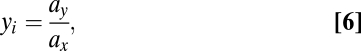where a_r, a_x, and a_y are allometric constants and m_b is the body size of basal species (35). The allometric scaling of each of these rates allows us to simplify the system and avoid an overabundance of parameters (27, 34). We use the following set of parameters: e_ij = 0.85, K = 1, m_b = 1, a_r = 1, a_x = 0.2227, and a_y = 1.7816 (all consumers are simulated as invertebrate carnivores). For the numerical integration, we use Hindmarsh's ordinary differential equation (ODE) solver LSODE.

Compartment Identification.

We identify the compartments within food webs by optimizing a quality function called modularity that provides a measure for the density of interactions within compartments compared with that between compartments (28). Modularity optimization has been shown to be a very successful approach to the search of compartments (also called communities or modules) in a wide variety of complex networks (29).

The modularity M (ℙ) of a partition ℙ of a network is defined as the fraction of interactions within compartments minus the expected fraction of such interactions (28). The expected fraction of interactions within compartments is evaluated assuming that the probability that species i and j are connected is k_ik_j/2L, where k_i is the number of interactions of node i and L is the total number of interactions in the network. Therefore, the modularity (28) is

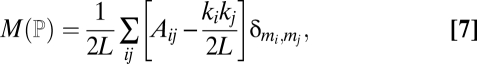where A is the adjacency matrix of the network (that is, A_ij = 1 if there is an interaction between i and j and A_ij = 0 otherwise), m_i is the compartment of species i, and δ is Kronecker's delta (δ_a,b = 1 if a = b and δ_a,b = 0 otherwise).

Modularity is high for “meaningful” partitions of a network into compartments and zero for random (typical) partitions (28). Although this modularity function does not explicitly take into account the directionality of trophic interactions, it has been recently used to successfully identify ecologically relevant compartments in food webs (11) and mutualistic networks (36).

Measuring Correlation Between Compartmentalization and Whole Food-Web Persistence.

To measure the relationship between compartmentalization and whole food-web persistence, we perform a multivariate linear regression to simultaneously control for the compartmentalization and connectance of the model food webs. There are thus two explanatory variables in our analysis, the connectance C and compartmentalization, measured by modularity M.

The multivariate model takes the form

where is the fractional persistence of the food web in the dynamic simulation, α is a constant, ε is the residual error, and the slopes β and γ measure the influence of connectance and compartmentalization, respectively.

One can assess the importance, in terms of predicting power, of a particular explanatory variable by examining the partial residuals of the model controlling for all other explanatory variables (37). If the residuals r of the model are given by

where , , and are the least-squares estimates from Eq. 8, the partial residuals corresponding to modularity M are defined as

In our case, the partial residuals can be understood as the contribution of compartmentalization to overall persistence as they capture the component not explained by either baseline persistence or connectance. To visualize the magnitude and direction of the effect of modularity M on overall persistence P, we therefore plot the partial residuals against the modularity in Fig. 2. The same can be seen for connectance C in SI Materials and Methods, Section S2.

Quantifying the Within-Compartment Response to Species Eliminations.

We wish to determine whether the effects of the intentional extinction of a species tend to be transmitted locally or distantly within a food web and whether the potentially cascading effects occur more or less rapidly. We quantify these aspects in two different fashions: the number of within-compartment extinctions and the time at which those within-compartment extinctions occur.

Number of Within-Compartment Extinctions.

We can count the number of extinctions that occur within the same compartment as an eliminated species i in the manipulated simulation (i.e., the simulation in which i was intentionally eliminated). We compare this value to that expected given a random null hypothesis with the same total number of extinctions (i.e., irrespective of whether they occur in the same compartment or not), the same number of compartments, and the same compartment sizes as observed (see SI Materials and Methods, Section S3 and Fig. S2 for more details of this randomization procedure and a schematic figure).

We then calculate the z -score

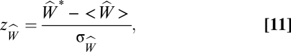where is the average number in an ensemble of randomizations and σ_W is the SD of the same quantity. To provide a baseline, we then count the number of extinctions W* in the unmanipulated simulation (i.e., the simulation in which species i was not intentionally eliminated). We calculate z_W in the same manner. To quantify the overall effect of compartmentalization, we compute 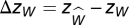. The value Δz_w can be thought of as the relative number of extinctions in the manipulated simulation compared with the unmanipulated simulation. If Δz_w > 0, extinctions that occur as a result of the species elimination have a greater tendency to occur in the same compartment as the eliminated species.

Time of Within-Compartment Extinctions.

We conduct the same analysis as above but, instead of the number of extinctions W*, we calculate the average time of extinction and T* for extinctions that occur in the same compartment as the eliminated species for the unmanipulated and manipulated simulations, respectively. We then compute , where and z_T are defined as above. The value Δz_T can be thought of as the relative time to extinction of extinctions in the manipulated simulation compared with those in the unmanipulated simulation. If Δz_T < 0, extinctions that occur in the same compartment as the eliminated species have a greater tendency to occur more rapidly.

Quantifying the Location of Cascading Extinctions.

To estimate how compartmentalization helps us understand which species extinctions are likely to occur after a previous extinction, we perform the following analysis, similar to that outlined above. We wish to determine if the effects of an initial species extinction tend to be transmitted locally or distantly within a food web. We quantify this effect with the number of consecutive extinction events that occur within the same compartment.

To calculate the number of consecutive extinctions within compartments, we first sort species according to the time of their extinction in the dynamic simulation. We then count the number of consecutive extinctions in which both species are from the same compartment.

We define the tendency of consecutive, within-compartment extinctions as

where is the average number of consecutive extinctions within compartments in an ensemble of randomizations and is the SD of the same quantity. The value quantifies the relative extinction tendency of species in the same compartment after a species i that has gone extinct.

We repeat this analysis but with other such observables. These include the number of consecutive extinctions between (i) directly connected species, D*; (ii) directly connected species within the same compartment, ; and (iii) nondirectly connected species within the same compartment, . Note that for any given simulation .

References

- 1.Elton CS. Ecology of Invasions by Animals and Plants. London: Chapman & Hall; 1958. [Google Scholar]
- 2.Hutchinson GE. Homage to Santa Rosalia or why are there so many kinds of animals? Am Nat. 1959;93:145–159. [Google Scholar]
- 3.May RM. Will a large complex system be stable? Nature. 1972;238:413–414. doi: 10.1038/238413a0. [DOI] [PubMed] [Google Scholar]
- 4.May RM. Stability and Complexity in Model Ecosystems. Princeton: Princeton Univ Press; 1973. [PubMed] [Google Scholar]
- 5.Yodzis P. The stability of real ecosystems. Nature. 1981;289:674–676. [Google Scholar]
- 6.Pimm SL. Food Webs. 1st Ed. Chicago: Univ of Chicago Press; 2002. [Google Scholar]
- 7.Gross T, Rudolf L, Levin SA, Dieckmann U. Generalized models reveal stabilizing factors in food webs. Science. 2009;325:747–750. doi: 10.1126/science.1173536. [DOI] [PubMed] [Google Scholar]
- 8.Girvan M, Newman MEJ. Community structure in social and biological networks. Proc Natl Acad Sci USA. 2002;99:7821–7826. doi: 10.1073/pnas.122653799. [DOI] [PMC free article] [PubMed] [Google Scholar]
- 9.Krause AE, Frank KA, Mason DM, Ulanowicz RE, Taylor WW. Compartments revealed in food-web structure. Nature. 2003;426:282–285. doi: 10.1038/nature02115. [DOI] [PubMed] [Google Scholar]
- 10.Allesina S, Pascual M. Food web models: A plea for groups. Ecol Lett. 2009;12:652–662. doi: 10.1111/j.1461-0248.2009.01321.x. [DOI] [PubMed] [Google Scholar]
- 11.Rezende EL, Albert EM, Fortuna MA, Bascompte J. Compartments in a marine food web associated with phylogeny, body mass, and habitat structure. Ecol Lett. 2009;12:779–788. doi: 10.1111/j.1461-0248.2009.01327.x. [DOI] [PubMed] [Google Scholar]
- 12.Guimerà R, et al. Origin of compartmentalization in food webs. Ecology. 2010;91:2941–2951. doi: 10.1890/09-1175.1. [DOI] [PubMed] [Google Scholar]
- 13.Pimm SL. The structure of food webs. Theor Popul Biol. 1979;16:144–158. doi: 10.1016/0040-5809(79)90010-8. [DOI] [PubMed] [Google Scholar]
- 14.Solow AR, Costello C, Beet AR. On an early result on stability and complexity. Am Nat. 1999;154:587–588. doi: 10.1086/303265. [DOI] [PubMed] [Google Scholar]
- 15.Murdoch WW, Walde SJ. Analysis of insect population dynamics. In: Grubb PJ, Whittaker JB, editors. Towards a More Exact Ecology. Oxford: Blackwell; 1989. pp. 113–140. [Google Scholar]
- 16.de Ruiter PC, Neutel AM, Moore JC. Energetics, patterns of interaction strengths, and stability in real ecosystems. Science. 1995;269:1257–1260. doi: 10.1126/science.269.5228.1257. [DOI] [PubMed] [Google Scholar]
- 17.Murdoch WW, et al. Single-species models for many-species food webs. Nature. 2002;417:541–543. doi: 10.1038/417541a. [DOI] [PubMed] [Google Scholar]
- 18.Rozdilsky ID, Stone L, Solow A. The effects of interaction compartments on stability for competitive systems. J Theor Biol. 2004;227:277–282. doi: 10.1016/j.jtbi.2003.11.007. [DOI] [PubMed] [Google Scholar]
- 19.Teng J, McCann KS. Dynamics of compartmented and reticulate food webs in relation to energetic flows. Am Nat. 2004;164:85–100. doi: 10.1086/421723. [DOI] [PubMed] [Google Scholar]
- 20.Pascual M, Dunne JA, editors. Ecological Networks: Linking Structure to Dynamics in Food Webs. Oxford: Oxford Univ Press; 2006. [Google Scholar]
- 21.Thébault E, Fontaine C. Stability of ecological communities and the architecture of mutualistic and trophic networks. Science. 2010;329:853–856. doi: 10.1126/science.1188321. [DOI] [PubMed] [Google Scholar]
- 22.Williams RJ, Martinez ND. Simple rules yield complex food webs. Nature. 2000;404:180–183. doi: 10.1038/35004572. [DOI] [PubMed] [Google Scholar]
- 23.Stouffer DB, Camacho J, Guimerà R, Ng CA, Amaral LAN. Quantitative patterns in the structure of model and empirical food webs. Ecology. 2005;86:1301–1311. [Google Scholar]
- 24.Stouffer DB, Camacho J, Amaral LAN. A robust measure of food web intervality. Proc Natl Acad Sci USA. 2006;103:19015–19020. doi: 10.1073/pnas.0603844103. [DOI] [PMC free article] [PubMed] [Google Scholar]
- 25.Williams RJ, Martinez ND. Success and its limits among structural models of complex food webs. J Anim Ecol. 2008;77:512–519. doi: 10.1111/j.1365-2656.2008.01362.x. [DOI] [PubMed] [Google Scholar]
- 26.Yodzis P, Innes S. Body size and consumer-resource dynamics. Am Nat. 1992;139:1151–1175. [Google Scholar]
- 27.Brose U, Williams RJ, Martinez ND. Allometric scaling enhances stability in complex food webs. Ecol Lett. 2006;9:1228–1236. doi: 10.1111/j.1461-0248.2006.00978.x. [DOI] [PubMed] [Google Scholar]
- 28.Newman MEJ, Girvan M. Finding and evaluating community structure in networks. Phys Rev E Stat Nonlin Soft Matter Phys. 2004;69:026113. doi: 10.1103/PhysRevE.69.026113. [DOI] [PubMed] [Google Scholar]
- 29.Guimerà R, Nunes Amaral LA. Functional cartography of complex metabolic networks. Nature. 2005;433:895–900. doi: 10.1038/nature03288. [DOI] [PMC free article] [PubMed] [Google Scholar]
- 30.Dunne JA, Williams RJ, Martinez ND. Network structure and biodiversity loss in food webs: Robustness increases with connectance. Ecol Lett. 2002;5:559–567. [Google Scholar]
- 31.Berlow EL, et al. Simple prediction of interaction strengths in complex food webs. Proc Natl Acad Sci USA. 2009;106:187–191. doi: 10.1073/pnas.0806823106. [DOI] [PMC free article] [PubMed] [Google Scholar]
- 32.May RM, Levin SA, Sugihara G. Complex systems: Ecology for bankers. Nature. 2008;451:893–895. doi: 10.1038/451893a. [DOI] [PubMed] [Google Scholar]
- 33.Stouffer DB, Bascompte J. Understanding food-web persistence from local to global scales. Ecol Lett. 2010;13:154–161. doi: 10.1111/j.1461-0248.2009.01407.x. [DOI] [PubMed] [Google Scholar]
- 34.Williams RJ. Effects of network and dynamical model structure on species persistence in large model food webs. Theor Ecol. 2008;1:141–151. [Google Scholar]
- 35.Brose U, et al. Consumer-resource body-size relationships in natural food webs. Ecology. 2006;87:2411–2417. doi: 10.1890/0012-9658(2006)87[2411:cbrinf]2.0.co;2. [DOI] [PubMed] [Google Scholar]
- 36.Oleson JM, Bascompte J, Dupont YL, Jordano P. The modularity of pollination networks. Proc Natl Acad Sci USA. 2007;104:19891–19896. doi: 10.1073/pnas.0706375104. [DOI] [PMC free article] [PubMed] [Google Scholar]
- 37.Larsen WA, McCleary SJ. The use of partial residual plots in regression analysis. Technometrics. 1972;14:781–790. [Google Scholar]
Associated Data
This section collects any data citations, data availability statements, or supplementary materials included in this article.