Stable linkage disequilibrium owing to sexual antagonism

Abstract

Linkage disequilibrium (LD) is an association between genetic loci that is typically transient. Here, we identify a previously overlooked cause of stable LD that may be pervasive: sexual antagonism. This form of selection produces unequal allele frequencies in males and females each generation, which upon admixture at fertilization give rise to an excess of haplotypes that couple male-beneficial with male-beneficial and female-beneficial with female-beneficial alleles. Under sexual antagonism, LD is obtained for all recombination frequencies in the absence of epistasis. The extent of LD is highest at low recombination and for stronger selection. We provide a partition of the total LD into distinct components and compare our result for sexual antagonism with Li and Nei's model of LD owing to population subdivision. Given the frequent observation of sexually antagonistic selection in natural populations and the number of traits that are often involved, these results suggest a major contribution of sexual antagonism to genomic structure.

1. Introduction

Linkage disequilibrium (LD) is a covariance between genetic loci that develops for various reasons including epistatic selection, drift, mutation and population structure [1]. LD may be transient or permanent, depending on which of these causes is responsible. Most instances of LD are transient because recombination randomly assigns alleles into gametes each generation. Unless the cause of LD is persistent, the association between loci is expected to decline geometrically over successive generations [2].

There are three known causes of stable LD. The first is epistatic interaction among loci [2–4]. Under this scenario, the fitness of an allele or genotype at one locus depends on the state of the second locus. This favours particular allelic combinations, which generate a statistical association between loci. Provided that selection maintains allelic variation at both loci, epistasis ensures that LD persists. Second, if fitness is determined multiplicatively across two overdominant loci that are sufficiently tightly linked, then a polymorphic equilibrium is necessarily accompanied by LD [5]. Third, permanent LD is possible in a metapopulation owing to allele frequency differences between subpopulations [6]. In fact, LD is expected in subdivided populations because linkage equilibrium requires the restrictive condition of equal allele frequencies in all subpopulations at one or both loci. LD persists provided that genetic variation is maintained in at least one subpopulation (or different combinations of alleles are fixed in different subpopulations).

In this paper, we identify sexual antagonism as a previously overlooked cause of permanent LD. Sexually antagonistic selection occurs when males and females have different phenotypic optima [7,8] and causes genotype frequencies in the male and female population to differ from each other after selection. Theoretically, sexual antagonism can maintain polymorphism [9]; empirically, sexually antagonistic selection is common [10] and sexually antagonistic fitness variation is prevalent in natural and laboratory populations [11–17]. Thus, for sexual antagonism, not only are the elements to produce stable LD in place, they are in abundance.

2. Model and results

We consider a model of two genetic loci with two alleles segregating at each: A₁ and A₂, B₁ and B₂. Let x_i and y_j be the frequencies of the ith and jth haplotypes in eggs and sperm, respectively, such that: x₁, y₁ are the frequencies of the A₁B₁ haplotype; x₂, y₂ the frequencies of the A₁B₂ haplotype; x₃, y₃ the frequencies of the A₂B₁ haplotype; and x₄, y₄ the frequencies of the A₂B₂ haplotype. We arrange the haplotype frequencies in eggs and sperm in vectors x and y, respectively (henceforth, lower-case bold letters represent vectors). Let p_x and p_y be the frequency of the A₁ allele in eggs and sperm and q_x and q_y be the frequency of the B₁ allele in eggs and sperm, respectively, calculated as p_ξ = ξ₁ + ξ₂ and q_ξ = ξ₁ + ξ₃, with ξ ∈ {x,y}.

Let genotypes A₁A₁, A₁A₂ and A₂A₂ have fitness u_1f = 1 − s_f, u_2f = 1 − h_fs_f and u_3f =1 in females, and u_1m = 1, u_2m = 1 − h_ms_m and u_3m = 1 − s_m in males, where 0 ≤ s ≤ 1. Fitness at the B locus, v_lχ with χ ∈ {f, m}, is parametrized in an analogous manner (table 1). For simplicity we assume that the allelic effects are additive at both loci (h_χ = 1/2), which guarantees opposing directional selection in the two sexes. We assume that the fitness of a zygote results from the product of the fitness values at each locus. Thus, w_ijχ = u_kχ v_lχ, where k and l ∈ {1, 2, 3}, is the fitness of a zygote of sex χ that results from the union of the ith egg and jth sperm haplotype (table 2). This assumption eliminates multiplicative epistasis within sexes by rendering the contributions of both loci independent from one another [18]. We arrange the fitness values for females and males in matrices W_f = (w_ijf) and W_m = (w_ijm). Given our assumptions, the number of different fitness values reduces to six (table 2b).

Table 1.

Genetic and fitness parametrization for males and females. (Recombination occurs between genes with frequency = r.)

	A1A1	A1A2	A2A2	B1B1	B1B2	B2B2
males	1	1 – 1/2 sm	1 – sm	1	1 – 1/2 sm	1 – sm
females	1 – sf	1 – 1/2 sf	1	1 – sf	1 – 1/2 sf	1

Table 2.

Fitness and frequencies of genotypes. (Female fitness is chosen for illustration, but a similar table can easily be drawn for males. The depiction in (a) shows the haplotype contributions from each parent to the diploid genotype; in (b), the two-locus diploid genotypes are decomposed into their single-locus components to show more clearly the contribution of each locus to fitness.)

(a)	A1B1	A1B2	A2B1	A2B2
A1B1	w11f, x1y1	w12f, x1y2	w13f, x1y3	w14f, x1y4
A1B2	w21f, x2y1	w22f, x2y2	w23f, x2y3	w24f, x2y4
A2B1	w31f, x3y1	w32f, x3y2	w33f, x3y3	w34f, x3y4
A2B2	w41f, x4y1	w42f, x4y2	w43f, x4y3	w44f, x4y4

(b)	B1B1	B1B2	B2B2
A1A1	(1 – sf)2, x1y1	(1 – sf) (1 – 1/2sf), x1y2 + x2y1	(1 – sf), x2y2
A1A2	(1 – sf) (1 – 1/2sf), x1y3 + x3y1	(1 – 1/2sf)2, x1y4 + x4y1 + x2y3 + x3y2	(1 – 1/2sf), x2y4 + x4y2
A2A2	(1 – sf), x3y3	(1 – 1/2sf), x3y4 + x4y3	1, x4y4

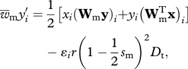
The frequency of haplotype i in eggs and sperm after one generation is

2.1a

and

2.1b

where and are the mean fitness of females and males, respectively (defined as ), r is the recombination rate between loci, ɛ_i provides the sign of the LD factor (ɛ_i is equal to 1 when i = 1,4 and −1 when i = 2,3) and D_t is the LD in the population.

When the selection regime is the same in both sexes, gametic haplotype frequencies are sex-independent (x_i = y_i) and D_t takes the familiar form D_t = x₁x₄ − x₂x₃. However, with sex-specific selection, D_t must be calculated as

2.2

When selection differs between the sexes, gametic haplotype frequencies depend on sex-specific allele frequencies at the two loci and the LD in eggs and sperm:

2.3

where

2.4

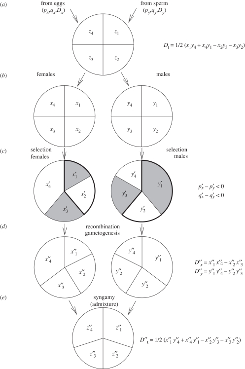
[2,17]. The flow of genes through populations is schematized in figure 1.

Figure 1.

Schematic depiction of alleles and haplotypes moving through a population over one generation. Each circle represents a gene pool at a different stage of the life cycle with the haplotype frequencies shown as areas within it. The cycle begins with sex-specific allele frequencies, haplotype frequencies and linkage disequilibrium values in parental gametes and ends with values of each owing to selection and recombination one generation later. Total linkage disequilibrium, D_t, is measured in the zygotes in each generation. (a) Diploid zygotes are formed from the random union of gametes and have total linkage disequilibrium D_t. (b) Juveniles are assigned to sexes. (c) Males and females experience sexually antagonistic selection, which favours alternate alleles at each locus in the two sexes. p′ corresponds to the thick line portions and q′ corresponds to the filled portions. This produces frequencies of p′_x and q′_x in females and p′_y and q′_y in males. (d) Recombination takes place between loci and haploid gametes are produced by meiosis. LD in the gametes is D″_x and D″_y. (e) The gametes are then united at random to form a new generation of zygotes. The linkage disequilibrium in these newly formed zygotes is D″_t = 1/2(D″_x + D″_y) + 1/2 (p′_x − p′_y)(q′_x − q′_y).

Substituting equation (2.3) into equation (2.2) and simplifying yield

2.5

where the second term on the right is equal to twice the covariance between p and q, 2 Cov(p,q); thus,

2.6

which provides a neat partition of the total LD generated by sexually antagonistic selection into two components, namely the average LD in gametes and the covariance between the allele frequencies at each locus.

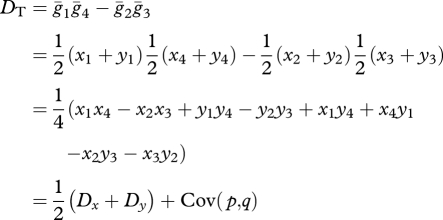
Equation (2.6) is similar in form to Nei & Li's [19] eqn (5) (D_T = 1/2 (D_x + D_y) + Cov(p,q)) for LD in a subdivided population. This formal similarity allows an interesting interpretation of our result. The two sexes, with their differing ecologies, physiologies and selection regimes [20], are effectively distinct subpopulations that freely exchange migrants from one generation to the next. The appendix explores the close analogy between our model and the model of Li & Nei ([6]; see also [19]).

We are interested in LD at a stable polymorphic equilibrium , i.e. . Calculating equilibrium haplotype frequencies analytically, even with our simplifying assumptions, proved too complex. Instead, we carried out numerical analysis of the recursions in equation (2.1) to determine the equilibrium points for different coefficients of selection s_f and s_m. When the equilibrium was polymorphic, we calculated the LD value for each pair (s_f, s_m) and for different values of recombination, r.

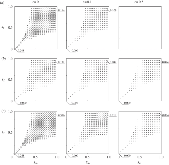
Figure 2 presents LD at polymorphic equilibria broken down into its components: and . LD is present at equilibrium for any value of r including free recombination (r = 1/2) (figure 2c). While the LD in gametes is absent at equilibrium when there is free recombination (figure 2a), the covariance between allele frequencies remains positive regardless of the recombination rate (figure 2b). Therefore, D_t remains positive.

Figure 2.

Linkage disequilibrium and its components for various recombination frequencies and selective strengths. LD is represented by the area of the circle at any given point (s_m, s_f) in the parameter space. The axes of each plot are the selection coefficient in males s_m (x-axis) and females s_f (y-axis). Recombination rate, r, differs for each column, increasing from left to right. (a) Average LD in gametes 1/2 (D_x + D_y). (b) Twice covariance between allele frequencies, 2 Cov(p,q). (c) Total LD, D_t, in zygotes.

LD increases with decreasing r (figure 2c). The covariance between allele frequencies, however, is less sensitive to r than the LD in gametes (figure 2a,b). For low r, the LD in gametes is the major contributor to D_t, whereas the covariance between allele frequencies becomes the major contributor for high r. The transition from being the major contributor to being the major contributor happens in the range of values between r = 0.1 and r = 0.3 (figure 3).

Figure 3.

Contribution to the total LD of the covariance between allele frequencies component relative to the LD in gametes component. The area of each circle represents the coefficient 4 Cov(p,q)/(D_x + D_y). Filled circles represent the case in which 1/2 (D_x + D_y) > 2 Cov(p,q), while empty circles represent the case in which 1/2 (D_x + D_y) < 2 Cov(p,q). The axes of each plot are the selection coefficient in males s_m (x-axis) and females s_f (y-axis). Recombination rate, r, differs for each column, increasing from left to right. (a) r = 0.1; (b) r = 0.2; (c) r =0.3.

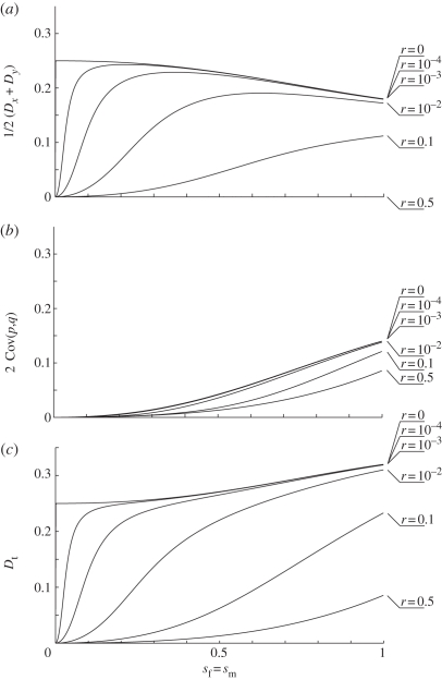
Finally, LD increases with strength of selection (figures 2 and 4c). This is not always the case for both of its components. It is always true for the covariance between allele frequencies (figure 4b). It is also true for the LD in gametes when the recombination rate is high (r > 0.1 in the symmetric example provided in figure 4a). When the recombination rate is low (r < 0.01 in the symmetric example provided in figure 4a), however, LD in gametes initially increases with strength of selection but then decreases at higher selection strengths (figure 4a).

Figure 4.

Linkage disequilibrium and its components as a function of selection strength for the particular case in which s_m = s_f. Each line represents the stable LD for different recombination rate values, indicated next to the line to the right of each figure. The axes in each plot are the selection coefficient s_m = s_f (x-axis) and the LD or its component (y-axis). The first row (a) corresponds to the average LD in gametes 1/2 (D_x + D_y). The second row (b) corresponds to the covariance between allele frequencies. The third row (c) corresponds to the total LD, D_t, in zygotes.

3. Discussion

The ultimate source of LD in our model is admixture between two gene pools with differing allele frequencies. Sexual antagonism results in a higher frequency of male beneficial alleles in sperm and of female beneficial alleles in eggs. Fertilization admixes these distinct gene pools and thereby generates LD in zygotes while homogenizing allele frequencies between the sexes (figure 1a). Whereas one-time admixture between geographically diverged populations produces transient LD that declines through subsequent generations, in our model, admixture between divergent subpopulations is recurrent because sexual antagonism alters the allele frequencies in opposing directions every generation. Therefore, permanent LD is maintained.

Equation (2.6) invites some further interpretation. This equation partitions D_t into two components: 2 Cov(p,q) represents the contribution to LD from sex differences in allele frequencies arising from sexually antagonistic selection in the immediately previous generation, whereas 1/2(D_x + D_y) represents accumulated LD from earlier generations. LD in gametes accumulates because of the correlated history of alleles at the two loci. When there is free recombination between maternally inherited and paternally inherited haplotypes, there is no correlation in the histories of the alleles at the two loci (whether they were present in the same or different sex) beyond the immediately preceding generation; further, the covariance between loci produced by admixture is erased by one round of free recombination; thus, D_x, D_y are expected to be zero at equilibrium. When recombination is less than 50 per cent, the histories of the alleles at the two loci in earlier generations are correlated and some of the LD produced by admixture in zygotes persists into the gametes, both of which make D_x, D_y ≠ 0 at equilibrium.

Sex-specific selection does not directly produce LD within a sex. The multiplicative fitness assumption precludes this. For instance, a population of zygotes in linkage equilibrium that then undergoes sexually antagonistic selection produces gametes with zero LD. Sexual antagonism is, however, indirectly responsible for the LD that results after admixture by virtue of its effect on the second term of equation (2.6). This term results from admixing sperm and egg gene pools, which are made unequal by sexual antagonism.

Selection that does not protect polymorphism cannot stabilize LD. Other selective causes of permanent LD considered in §1 (epistatic interactions, multiplicative fitness at two overdominant loci) require special—perhaps extraordinary—circumstances. For instance, fitness variance owing to epistatic interactions exists, but whether epistasis is responsible for the maintenance of this variation is unknown. In order for two overdominant loci to maintain LD, the recombination rate must be less than the marginal segregation load of the population [5], which for selection coefficients under 50 per cent requires that the recombination rate be less than approximately 0.0625. Allele frequency differences among subpopulations are degraded through time by migration unless there is subpopulation-specific selection. The subdivision of populations into two sexes and sexually antagonistic selection are both common [10]. Therefore, the prerequisites for permanent LD under sexual antagonism are present in many natural populations.

However, two theoretical considerations may lessen the occurrence of LD caused by sexual antagonism. The first is the possibility for conflict resolution—i.e. sexual dimorphism [21]. Should a sexually antagonistic locus evolve sex-limited expression, the allele that is favoured in the expressing sex is expected to fix, thus eliminating variation and precluding LD. The time scale over which intralocus conflict operates—and therefore the likelihood of developing permanent LD—is currently unknown: if conflicts are constantly arising but then are quickly (on an evolutionary time scale) resolved by the evolution of dimorphism, the build-up of LD should be minor; if polymorphisms are maintained for longer periods, then LD has more time to develop and should be more widespread. Dating the age of alleles at sexually antagonistic loci could potentially shed light on this question. Such loci have recently been identified by Innocenti & Morrow [22]. The second consideration draws on the work of Turelli & Barton [23]. They showed that at most two loci could remain polymorphic owing to sexually antagonistic selection. Their model makes assumptions that are relaxed in our model. Specifically, Turelli & Barton [23] considered a model in which loosely linked loci determined a single trait subject to weak sexually antagonistic selection. Our model is agnostic about the number of traits subject to sexually antagonistic selection, permits any value of recombination and considers strong as well as weak selection. Future analyses with more than two loci should explore the potential to maintain large amounts of LD.

LD will be created between any two loci that are polymorphic for sexually antagonistic alleles, even for genes that code for different traits. Multi-locus models may introduce still further higher order associations among loci that are not accounted for in our two-locus model [24]. Based on our theoretical results, we expect there to be wide-ranging multi-locus association in genomes that has not yet been examined. Such associations complicate any attempt to find the genes responsible for phenotypes of interest because the standard approach relies on there being a statistical association between the two. With the kind of LD we find accompanying sexual antagonism, we expect that all sexually antagonistic loci show a statistical association with all sexually antagonistic traits.

The division of the population into two sexes that are subject to sex-specific selection is just one way that a gene pool could be subdivided into groups that undergo differential selection. Regular admixture between such subgroups will generate persistent LD [6]. As an example, suppose that a population consists of a mixture of vegetarians and meat-eaters but the two groups sometimes intermarry and children have some independence in the diet they choose to adopt. If the different diets result in differential selection and allele frequency differences between reproductive vegetarians and reproductive meat-eaters, then admixture of these gene pools in their offspring will be a source of LD. This LD arises because of a correlation in the selective forces acting at different loci in the two subpopulations. This hypothetical example suggests that the existence of differential selection at two loci can be a source of persistent LD whenever the selective ‘environments’ at two loci are correlated.

Appendix A

The discrepancy between our theoretical value of total LD, D_t = 1/2 (D_x + D_y) + 2 Cov(p,q), and Nei & Li's [19] value, D_T = 1/2 (D_x + D_y) + Cov(p,q), arises from the way we define LD. Standard two-locus models that lack sex differences obscure the fact that there are two possible choices. One interpretation is that LD is the quantity that must be added or subtracted to the products of allele frequencies to give the correct haplotype frequencies. An example of this can be seen in our equation (2.3). A second interpretation is that LD measures the difference in frequency between the different kinds of double heterozygotes. This difference is evolutionarily relevant because only in double heterozygotes does recombination have a chance to alter haplotype frequencies and break down the association between loci. Not surprisingly, this quantity appears in the recursion equations for haplotype frequencies in our model (equations (2.1) and (2.2)). In a model that lacks sexes or subpopulations, the two interpretations take the same value: g₁g₄−g₂g₃, where g_i is the frequency of the ith haplotype in the total population. With the population structure that our model and Nei & Li's [19] model introduce, these two interpretations are no longer equivalent. They are, however, mathematically connected as we show below.

Nei & Li [19] average the ith haplotype frequencies across subpopulations to obtain the population-wide frequency, . Using the terminology from our model, . They then expand , which produces a value, D_T, which must be added to the product of population-wide allele frequencies to produce the average haplotype frequencies ([19], eqn (5)):

A 1

Finally, etc.

In our model, we take D_t to be half the difference between coupling and repulsion double heterozygotes, a quantity that is sitting in equation (2.1):

A 2

(equations (2.2) and (2.6)).

The relation between Nei & Li's [19] D_T and our D_t can be seen in the third step of equation (A 1). This can be expressed as:

A 3

The two interpretations of LD, D_T and D_t, differ by the magnitude of Cov(p,q) but essentially capture the same phenomenon. Nei & Li's [19] interpretation sticks closer to what would probably be measured empirically and to the definition set out by the originators of the term:

The equations … imply that any time the gametic frequencies will deviate from the equilibrium frequencies by an amount D which is the product of the coupling gametic frequencies minus that of the repulsion gametic frequencies. D, thus defined, may be considered as a measure of linkage disequilibrium (italics in original; 2, p. 459).

However, our interpretation better captures the quantity that matters to the evolution of the haplotype frequencies [4] and follows the definition used by Crow & Kimura ([25], p. 197), namely ‘the difference in frequency between the two types of heterozygotes’.

References

- 1.Slatkin M. 2008. Linkage disequilibrium: understanding the evolutionary past and mapping the medical future. Nat. Rev. Genet. 9, 477–485 10.1038/nrg2361 (doi:10.1038/nrg2361) [DOI] [PMC free article] [PubMed] [Google Scholar]
- 2.Lewontin R. C., Kojima K. 1960. The evolutionary dynamics of complex polymorphisms. Evolution 14, 458–472 10.2307/2405995 (doi:10.2307/2405995) [DOI] [Google Scholar]
- 3.Fisher R. A. 1930. The genetical theory of natural selection. Oxford, UK: Clarendon Press [Google Scholar]
- 4.Kimura M. 1956. A model of a genetic system which leads to closer linkage by natural selection. Evolution 10, 278–287 10.2307/2406012 (doi:10.2307/2406012) [DOI] [Google Scholar]
- 5.Bodmer W. F., Felsenstein J. 1967. Linkage and selection: theoretical analysis of the deterministic two locus random mating model. Genetics 57, 237–265 [DOI] [PMC free article] [PubMed] [Google Scholar]
- 6.Li W. H., Nei M. 1974. Stable linkage disequilibrium without epistasis in a subdivided population. Theor. Popul. Biol. 6, 173–183 10.1016/0040-5809(74)90022-7 (doi:10.1016/0040-5809(74)90022-7) [DOI] [PubMed] [Google Scholar]
- 7.Bonduriansky R., Chenoweth S. F. 2009. Intralocus sexual conflict. Trends Ecol. Evol. 24, 280–288 10.1016/j.tree.2008.12.005 (doi:10.1016/j.tree.2008.12.005) [DOI] [PubMed] [Google Scholar]
- 8.Van Doorn G. S. 2009. Intralocus sexual conflict. Ann. NY Acad. Sci. 1168, 52–71 10.1111/j.1749-6632.2009.04573.x (doi:10.1111/j.1749-6632.2009.04573.x) [DOI] [PubMed] [Google Scholar]
- 9.Kidwell J. F., Clegg M. T., Stewart F. M., Prout T. 1977. Regions of stable equilibria for models of differential selection in the two sexes under random mating. Genetics 85, 171–183 [DOI] [PMC free article] [PubMed] [Google Scholar]
- 10.Cox R. M., Calsbeek R. 2009. Sexually antagonistic selection, sexual dimorphism, and the resolution of intralocus sexual conflict. Am. Nat. 173, 176–187 [DOI] [PubMed] [Google Scholar]
- 11.Chippindale A. K., Gibson J. R., Rice W. R. 2001. Negative genetic correlation for adult fitness between sexes reveals ontogenetic conflict in Drosophila. Proc. Natl Acad. Sci. USA 98, 1671–1675 10.1073/pnas.041378098 (doi:10.1073/pnas.041378098) [DOI] [PMC free article] [PubMed] [Google Scholar]
- 12.Gibson J. R., Chippindale A. K., Rice W. R. 2002. The X chromosome is a hot spot for sexually antagonistic fitness variation. Proc. R. Soc. Lond. B 269, 499–505 10.1098/rspb.2001.1863 (doi:10.1098/rspb.2001.1863) [DOI] [PMC free article] [PubMed] [Google Scholar]
- 13.Pischedda A., Chippindale A. K. 2006. Intralocus sexual conflict diminishes the benefits of sexual selection. PLoS Biol. 4, 2099–2103 [DOI] [PMC free article] [PubMed] [Google Scholar]
- 14.Brommer J. E., Kirkpatrick M., Qvarnström A., Gustafsson L. 2007. The intersexual genetic correlation for lifetime fitness in the wild and its implications for sexual selection. PLoS ONE 2, e744, 741–746 [DOI] [PMC free article] [PubMed] [Google Scholar]
- 15.Foerster K., Coulson T., Sheldon B. C., Pemberton J. M., Clutton-Brock T. H., Kruuk L. E. B. 2007. Sexually antagonistic genetic variation for fitness in red deer. Nature 447, 1107–1109 10.1038/nature05912 (doi:10.1038/nature05912) [DOI] [PubMed] [Google Scholar]
- 16.Prasad N. G., Bedhomme S., Day T., Chippindale A. K. 2007. An evolutionary cost of separate genders revealed by male-limited evolution. Am. Nat. 169, 29–37 [DOI] [PubMed] [Google Scholar]
- 17.Delcourt M., Blows M. W., Rundle H. D. 2009. Sexually antagonistic genetic variance for fitness in an ancestral and a novel environment. Proc. R. Soc. B 276, 2009–2014 10.1098/rspb.2008.1459 (doi:10.1098/rspb.2008.1459) [DOI] [PMC free article] [PubMed] [Google Scholar]
- 18.Karlin S. 1975. General two-locus selection models: some objectives, results and interpretations. Theor. Popul. Biol. 7, 364–398 10.1016/0040-5809(75)90025-8 (doi:10.1016/0040-5809(75)90025-8) [DOI] [PubMed] [Google Scholar]
- 19.Nei M., Li W. H. 1973. Linkage disequilibrium in subdivided populations. Genetics 75, 213–219 [DOI] [PMC free article] [PubMed] [Google Scholar]
- 20.Fairbairn D. J., Blankenhorn W. U., Székely T. 2007. Sex, size, and gender roles: evolutionary studies of sexual size dimorphism. Oxford, UK: Oxford University Press [Google Scholar]
- 21.Rice W. R. 1984. Sex chromosomes and the evolution of sexual dimorphism. Evolution 38, 735–742 10.2307/2408385 (doi:10.2307/2408385) [DOI] [PubMed] [Google Scholar]
- 22.Innocenti P., Morrow E. H. 2010. The sexually antagonistic genes of Drosophila melanogaster. PLoS Biol. 8, e1000335. 10.1371/journal.pbio.1000335 (doi:10.1371/journal.pbio.1000335) [DOI] [PMC free article] [PubMed] [Google Scholar]
- 23.Turelli M., Barton N. H. 2004. Polygenic variation maintained by balancing selection: pleiotropy, sex-dependent allelic effects and G×E interactions. Genetics 166, 1053–1079 10.1534/genetics.166.2.1053 (doi:10.1534/genetics.166.2.1053) [DOI] [PMC free article] [PubMed] [Google Scholar]
- 24.Franklin I., Lewontin R. C. 1970. Is the gene the unit of selection? Genetics 65, 707–734 [DOI] [PMC free article] [PubMed] [Google Scholar]
- 25.Crow J. F., Kimura M. 1970. An introduction to population genetics theory. New York, NY: Harper and Row [Google Scholar]