Hypoelastic Soft Tissues

Abstract

In Part I, a novel hypoelastic framework for soft-tissues was presented. One of the hallmarks of this new theory is that the well-known exponential behavior of soft-tissues arises consistently and spontaneously from the integration of a rate based formulation. In Part II, we examine the application of this framework to the problem of biaxial kinematics, which are common in experimental soft-tissue characterization. We confine our attention to an isotropic formulation in order to highlight the distinction between non-linearity and anisotropy. In order to provide a sound foundation for the membrane extension of our earlier hypoelastic framework, the kinematics and kinetics of in-plane biaxial extension are revisited, and some enhancements are provided. Specifically, the conventional stress-to-traction mapping for this boundary value problem is shown to violate the conservation of angular momentum. In response, we provide a corrected mapping. In addition, a novel means for applying loads to in-plane biaxial experiments is proposed. An isotropic, isochoric, hypoelastic, constitutive model is applied to an in-plane biaxial experiment done on glutaraldehyde treated bovine pericardium. The experiment is comprised of eight protocols that radially probe the biaxial plane. Considering its simplicity (two adjustable parameters) the model does a reasonably good job of describing the non-linear normal responses observed in these experimental data, which are more prevalent than are the anisotropic responses exhibited by this tissue.

1 Introduction

In-plane biaxial experiments constitute an important class of experiment used to study the mechanical response of soft biological tissues. In this paper, we re-examine this boundary value problem (BVP), bringing to it new insight. In particular, attention is given to the polar decomposition of the deformation gradient, the construction of kinematic rates from experimental data, and the mapping between stress and traction.

The isotropic hypoelastic model derived in part I [1] of this paper is modified for in-plane biaxial extension, and is then applied to experimental data obtained from the author’s (MSS) laboratory for glutaraldehyde treated bovine pericardium—a tissue commonly used in bioprosthetic heart valves [2,3]. This chemical treatment cross-links the tissue, making it stiffer, a by-product of reducing its immugenicity so as to mitigate a patient’s need for anticoagulation therapy. Our objective is to explore what this simple model is, and is not, capable of achieving. Application of the anisotropic composite model (also derived in part I) to this experimental data set will be the topic of a future paper.

It is a well established fact that pericardium is a membranous tissue strengthened with an anisotropic distribution of collagen fibers [4,5]. So why try to fit an isotropic model to an otherwise anisotropic material? The answer is two fold. First, as an aid to distinguish between whether a particular effect is non-linear in origin, or anisotropic in origin. And second, to get an order-of-magnitude sense as to the error that one would likely be making if one were to use the simpler isotropic model, especially in preliminary analyses where parameters are likely to be assigned via engineering judgment. It turns out that this simple two-parameter model does remarkably well at describing the general stress/strain response of pericardium, but there is room for improvement, especially in correctly predicting the shear response.

The paper is organized as follows. The next section reviews the kinematics of in-plane biaxial extension, with new expressions given for the stretch and rotation tensors. Section 3 investigates the stress-to-traction map for this BVP. It is shown that the classic map violates the conservation of angular momentum—a flaw that is corrected. Also presented is a novel idea for loading an in-plane specimen to achieve a larger region of nearly uniform stress at its center. Section 4 configures the isotropic, hypoelastic, constitutive model for membrane analysis. Section 5 applies this model to glutaraldehyde treated bovine pericardium. Section 6 provides a discussion of results, with Sec. 7 summarizing the paper. An Appendix describes a likelihood objective function that was used for parameter estimation, and the integration algorithm used herein.

2 Kinematics of In-Plane Biaxial Extension

Sacks [6] and Sacks & Sun [5] have written review articles on in-plane, biaxial, test methods used by experimentalists in the field of soft-tissue mechanics, and Humphrey [7] has dedicated a chapter to it in his book (Chp. 5). The discussion presented here provides a somewhat more detailed analysis of the polar decomposition of this deformation, and it addresses those rate related fields that are of interest when hypoelastic or viscoelastic constructions are to be employed.

Holzapfel & Ogden [8] have analyzed the in-plane biaxial BVP from the viewpoint of hyperelas-ticity. They have shown that this experiment, by itself, is insufficient to completely characterize a three-dimensional (3D), anisotropic, isochoric, hyperelastic solid; it is only sufficient to characterize an isotropic, isochoric, hyperelastic solid in 3-space. Additional experiments are needed for a complete 3D characterization of anisotropic materials; in particular, ones with a through-thickness shear component are suggested, like cross-plane simple shear. This does not diminish the importance of planar experiments to the overall process of parameter estimation; rather, they point out the need for experimentalists to develop complementary, novel, experimental capabilities, like those of Dokos et al. [9], so that complete 3D soft-tissue characterizations can become possible in the future.

In-plane biaxial experiments are, however, sufficient to completely characterize two-dimensional (2D) material models for membranes, and it is in this capacity that this BVP is utilized here.

2.1 Deformation

Consider a homogeneous deformation described by the BVP

$$x_1={\lambda }_1{X}_1+{\gamma }_1{X}_2,x_2={\gamma }_2{X}_1+{\gamma }_2{X}_2\text{and}{x}_3={\lambda }_3{X}_3,$$ (1)

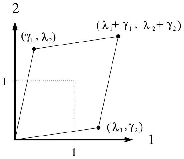
where coordinates (X₁,X₂,X₃) locate the initial position of a mass point, while the coordinate functions (x₁,x₂,x₃) locate its current position. Parameters λ_i and γ_i represent the stretch and shear components, respectively, of the planar deformation shown in Fig. 1. Shears arise naturally when testing soft tissues as their fibers attempt to align themselves with the principle loading directions by a shearing the softer matrix material betwixt them [10]. The kinematic parameters λ_i and γ_i are usually acquired via finite-element technology through an image tracking of markers fixed to the specimen [7,11,12].

Fig. 1.

Schematic of a biaxial extension with in-plane shear. A dotted square is deformed into a solid quadrilateral.

The deformation gradient F=∂ x_i/∂X_j e_i ⊗ e_j is the fundamental descriptor of deformation in hyperelastic material models, whose components for this deformation are

$$\mathbf{F}=\left[\begin{array}{ccc}{\lambda }_1& {\gamma }_1& 0\\ {\gamma }_2& {\lambda }_2& 0\\ 0& 0& {\lambda }_3\end{array}\right]\text{with}{\lambda }_3=\frac{1}{\mathrm{\Lambda }}\text{wherein}\mathrm{\Lambda }={\lambda }_1{\lambda }_2-{\gamma }_1{\gamma }_2,$$ (2)

where the stated expression for λ₃ follows from the isochoric constraint, detF = 1, which is a reasonable assumption to impose on most soft tissues [13]. Variable Λ denotes the areal stretch; it being the surface area in the current state divided by the surface area in the reference state.

By adopting the isochoric constraint, the spatial dimension of F, as it pertains to deformation (2), can be reduced from three dimensions down to two, allowing it and its inverse to be represented by

$$\mathbf{F}=\left[\begin{array}{ll}{\lambda }_1\hfill & {\gamma }_1\hfill \\ {\gamma }_2\hfill & {\lambda }_2\hfill \end{array}\right]\text{and}{\mathbf{F}}^{-1}=\frac{1}{\mathrm{\Lambda }}\left[\begin{array}{ll}{\lambda }_2\hfill & -{\gamma }_1\hfill \\ -{\gamma }_2\hfill & {\lambda }_1\hfill \end{array}\right],$$ (3)

where now the detF associates with a change in area, not a change in volume, i.e., detF = λ₁λ₂ − γ₁γ₂ = Λ.

2.2 Polar Decomposition

Added insight can be gained by considering a polar decomposition F = RU of the deformation (3). Let the rotation R take on a classic form of

$$\mathbf{R}=\left[\begin{array}{cc}\hfill cos\theta \hfill & \hfill -sin\theta \hfill \\ \hfill sin\theta \hfill & \hfill cos\theta \hfill \end{array}\right],$$ (4)

so that the sign of θ will be positive during counterclockwise rotations. This mandates that the right-stretch tensor U has components

$$\mathbf{U}=\left[\begin{array}{cc}\hfill {\lambda }_{1}cos\theta +{\gamma }_{2}sin\theta \hfill & \hfill {\gamma }_{1}cos\theta +{\lambda }_{2}sin\theta \hfill \\ \hfill {\gamma }_{2}cos\theta -{\lambda }_{1}sin\theta \hfill & \hfill {\lambda }_{2}cos\theta -{\gamma }_{1}sin\theta \hfill \end{array}\right].$$ (5)

From the symmetry of stretch (that is, U₁₂ = U₂₁) one determines that

$$\theta ={tan}^{-1}\left(\frac{{\gamma }_2-{\gamma }_1}{{\lambda }_1+{\lambda }_2}\right).$$ (6)

This allows the rotation to be re-expressed in terms of its primitive variables λ₁, λ₂, γ₁ and γ₂, i.e.,

$$\mathbf{R}=\frac{1}{\mathrm{\Xi }}\left[\begin{array}{cc}{\lambda }_1+{\lambda }_2& -({\gamma }_2-{\gamma }_1)\\ {\gamma }_2-{\gamma }_1& {\lambda }_1+{\lambda }_2\end{array}\right]\text{with}\mathrm{\Xi }=\sqrt{{({\lambda }_1+{\lambda }_2)}^2+{({\gamma }_2-{\gamma }_1)}^2},$$ (7)

where Ξ is the hypotenuse, λ₁ + λ₂ is the abscissa, and γ₂ − γ₁ is the ordinate of the triangle that tracks rigid-body rotation. This expression for the rotation R allows the right-stretch tensor to be rewritten as

$$\mathbf{U}=\frac{1}{\mathrm{\Xi }}\left[\begin{array}{cc}{\lambda }_1({\lambda }_1+{\lambda }_2)+{\gamma }_2({\gamma }_2-{\gamma }_1)& {\gamma }_1{\lambda }_1+{\gamma }_2{\lambda }_2\\ {\gamma }_1{\lambda }_1+{\gamma }_2{\lambda }_2& {\lambda }_2({\lambda }_1+{\lambda }_2)-{\gamma }_1({\gamma }_2-{\gamma }_1)\end{array}\right].$$ (8)

Components of the left-stretch tensor V = RUR^T = FR^T, and the two inverses U⁻¹ = F⁻¹R and V⁻¹ = RF⁻¹, can be gotten easily from above matrix formulæ.

2.3 Rates from Smoothing Splines

There are two kinematic rates from which all other kinematic rates can be derived; they are the velocity gradient L = ḞF⁻¹ and the rate of rotation Ω = ṘR⁻¹ = ṘR^T. As F is the fundamental descriptor for hyperelastic material models; likewise, L is the fundamental descriptor for hypoelastic and viscoelastic material models. Furthermore, as R is needed to account for rigid-body rotation in hyperelastic models, so too is Ω needed to account for the rate of rigid-body rotation in hypoelastic and viscoelastic models.

The four planar components of the deformation gradient F are the measured kinematic quantities in an in-plane biaxial experiment. Rates Ḟ and Ṙ must be derived from these four data streams. Because methods for the numeric differentiation of experimental data magnify noise within a data stream, and because these data streams tend to be noisy to begin with, it is vital in this application that one smooth the raw F_{i j} data streams in order to get meaningful estimates for the Ḟ_{i j}. These rates are gotten by differentiating the smoothing function, not the data themselves. A cubic B-spline built into the generalized cross-validatory (GCV) method of Woltring [14] was used to smooth our raw F_{i j} data.¹

From the smoothed data streams that now describe F and Ḟ, one can quantify the velocity gradient according to its definition, viz.,

$$\mathbf{L}=\stackrel{.}{\mathbf{F}}{\mathbf{F}}^{-1},\text{where}{\mathbf{F}}^{-1}=\frac{1}{\mathrm{\Lambda }}\left[\begin{array}{cc}{\lambda }_2& -{\gamma }_1\\ -{\gamma }_2& {\lambda }_1\end{array}\right]\text{and}\stackrel{.}{\mathbf{F}}=\left[\begin{array}{cc}{\stackrel{.}{\lambda }}_1& {\stackrel{.}{\gamma }}_1\\ {\stackrel{.}{\gamma }}_2& {\stackrel{.}{\lambda }}_2\end{array}\right],$$ (9)

recalling that Λ = λ₁λ₂ − γ₁γ₂. Furthermore, upon differentiating the rotation described in either Eq. (4 or 7), while utilizing the definition for the rate of rotation Ω = ṘR^T, one is lead to a simple result describing rate of rotation, i.e.,

$$\mathit{\Omega }=\stackrel{.}{\theta }\left[\begin{array}{cc}0& -1\\ 1& 0\end{array}\right],$$ (10)

where θ̇ = ((λ₁ + λ₂)(γ̇₂ − γ̇₁) − (γ₂ − γ₁)(λ̇₁ + λ̇₂)/((λ₁ + λ₂)² + (γ₂ − γ₁)²) is the time rate-of-change of the angular rotation θ defined in Eq. (6).

3 Kinetics of In-Plane Biaxial Extension

To compare predictions/correlations of a constitutive model with experimental data, it is not only necessary to be able to convert the displacements of an experiment into states of strain, it is also desirable to convert the tractions of an experiment into states of stress, when permissible. In this section, we first present the historical approach used to obtain stresses from tractions in a planar biaxial setting and show, in the presence of nonnegligible shears, that this mapping is in error. We then present a new map that obeys the conservation of angular momentum, and finish with a note on boundary conditions.

3.1 Historical Approach

The force df acting on an infinitesimal area dA₀ of surface with normal n₀ in the reference configuration obeys the mapping df = P · n₀ dA₀, where tensor P = P_{i j} e_i ⊗ e_j = JτF^−T is the first Piola-Kirchhoff stress, which is not symmetric; tensor τ is the Cauchy stress, which must be symmetric so as to conserve angular momentum; tensor T = Jτ is the symmetric Kirchhoff stress²; and scalar J = det F quantifies the change in volume taking place between the reference and current states, which is constrained to be one because of the isochoric assumption [16,17]. Consequently, there is no numeric difference between the stress measures of Cauchy and Kirchhoff in soft-tissue mechanics whenever the isochoric assumption is imposed.

The current stress-to-traction map used for in-plane biaxial extension has an assumed form of [5,7,18]

$$\frac{\text{d}\mathbf{f}}{{\text{d}A}_0}=\left\{\begin{array}{l}{\sigma }_1\\ 0\end{array}\right\}=\left[\begin{array}{cc}{P}_{11}& 0\\ 0& P_{22}\end{array}\right]\left\{\begin{array}{c}1\\ 0\end{array}\right\}\text{and}\frac{\text{d}\mathbf{f}}{{\text{d}A}_0}=\left\{\begin{array}{l}0\\ {\sigma }_2\end{array}\right\}=\left[\begin{array}{cc}{P}_{11}& 0\\ 0& P_{22}\end{array}\right]\left\{\begin{array}{c}0\\ 1\end{array}\right\},$$ (11)

where the engineering stresses σ_i are physical fields defined by

$${\sigma }_1=\frac{f_1}{{\ell }_2{\ell }_3}\text{and}{\sigma }_2=\frac{f_2}{{\ell }_1{\ell }_3},$$ (12)

with each f_i denoting an applied force acting in the ith direction, and each ℓ_i specifying a gage length measured along the i^th direction, with ℓ₃ quantifying the initial thickness of the test sample. Consequently, P₁₁ = σ₁ and P₂₂ = σ₂, provided that this assumed mapping is correct.

The Kirchhoff stress associated with this mapping has components

$$\mathbf{T}=\mathbf{P}{\mathbf{F}}^T=\left[\begin{array}{ll}{\lambda }_1{P}_{11}\hfill & {\gamma }_2{P}_{11}\hfill \\ {\gamma }_1{P}_{22}\hfill & {\lambda }_2{P}_{22}\hfill \end{array}\right].$$ (13)

This tensor must be symmetric because of the physical law that conserves angular momentum [16,17], consequently

$$T_{21}={\gamma }_1{P}_{22}={\gamma }_2{P}_{11}=T_{12}\text{or}\text{equivalently}{\gamma }_1{\sigma }_2={\gamma }_2{\sigma }_1.$$ (14)

As a result, the two shears γ₁ and γ₂ cannot act independently whenever stresses relate to tractions according to the presumed mappings given in Eq. (11).

3.2 Experimental Assessment of Stress Constraint (14)

The Billiar-Sacks [19], in-plane, biaxial experiments done on aortic heart valves were run in load control at constant rates to targeted values of (protocol; σ₁: σ₂) 1;100:4, 2;100:50, 3;100:75, 4;100:100, 5;75:100, 6;50:100 and 7;17:100, with stresses being listed in kPa. These seven protocols were applied sequentially to a single specimen so that the fiber alignment would be the same for all protocols within a given data set. The 1-direction in their specimens aligned roughly with the mean fiber direction associated with the circumference of a leaflet, while the 2-direction was radial in orientation, normal to the mean fiber reinforcement. Their membrane tractions (forces per unit length) have been converted into stresses (forces per unit area) here by assigning a nominal tissue thickness ℓ₃ of 0.6 mm.

An examination of their experimental data for fresh leaflets excised from porcine, aortic, heart valves permits an experimental assessment of the angular momentum constraint specified in Eq. (14). The outcome of our assessment, using their data, is presented in Fig. 2. The shear components of the Kirchhoff stress, so defined, are on the order of 10% of their normal values. Such differences are significant. Obviously, T₁₂ ≠ T₂₁ throughout the entire loading history. They are not even remotely close. These data clearly demonstrate that the resulting constraint equation (14) for the conservation of angular momentum is violated, and therefore, the assumption that the stress-to-traction map stated in Eq. (11) is valid must be dismissed.

Fig. 2.

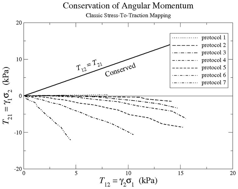
An assessment of constraint equation (14)—the solid line—for conserving angular momentum, as it applies to the experimental data of Billiar & Sacks [19] using the stress-to-traction mapping in Eq. (11). The solid line ought to be the experimental mean; obviously, it is not for these data. The magnitudes of these shear-stress components are about 10% of their associated normal-stress counterparts.

3.3 Tractions Revisited

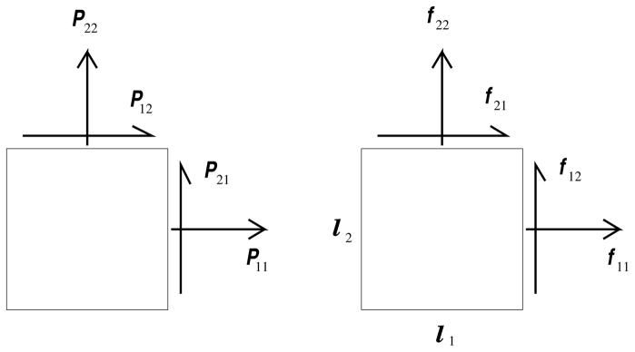
The data presented in Fig. 2 provide experimental evidence that the hypothesis that “The map given in Eq. (11) is physical.” must be rejected, being replaced by the more general map

$$\frac{\text{d}\mathbf{f}}{{\text{d}A}_0}=\left\{\begin{array}{l}{f}_{11}/{\ell }_2{\ell }_3\hfill \\ f_{12}/{\ell }_2{\ell }_3\hfill \end{array}\right\}=\left[\begin{array}{ll}{P}_{11}\hfill & P_{12}\hfill \\ P_{21}\hfill & P_{22}\hfill \end{array}\right]\left\{\begin{array}{l}1\hfill \\ 0\hfill \end{array}\right\}\text{and}\frac{\text{d}\mathbf{f}}{{\text{d}A}_0}=\left\{\begin{array}{l}{f}_{21}/{\ell }_1{\ell }_3\hfill \\ f_{22}/{\ell }_1{\ell }_3\hfill \end{array}\right\}=\left[\begin{array}{ll}{P}_{11}\hfill & P_{12}\hfill \\ P_{21}\hfill & P_{22}\hfill \end{array}\right]\left\{\begin{array}{l}0\hfill \\ 1\hfill \end{array}\right\},$$ (15)

as illustrated in Fig. 3. Here the experimentally applied tractions f₁ and f₂ have constituents

Fig. 3.

An illustration showing how the forces and gage lengths relate to the components of the first Piola-Kirchhoff stress. Notice that the corresponding shear indices are switched. For them to be the same, one would be relating the nominal stress components to the forces of traction instead of those belonging to the first Piola-Kirchhoff stress (cf. Ogden [16, pg. 153]).

$$f_1=f_{11}+f_{21}\text{and}{f}_2=f_{12}+f_{22},$$ (16)

where the i^th index of f_{i j} indicates the direction of the normal upon whose surface the traction is applied, while the j^th index indicates the direction that the force is applied.

It follows from Eq. (15) that the first Piola-Kirchhoff stress will now have components

$$\mathbf{P}=\left[\begin{array}{ll}{f}_{11}/{\ell }_2{\ell }_3\hfill & f_{21}/{\ell }_1{\ell }_3\hfill \\ f_{12}/{\ell }_2{\ell }_3\hfill & f_{22}/{\ell }_1{\ell }_3\hfill \end{array}\right],$$ (17)

allowing the Kirchhoff stress to be quantified according to

$$\mathbf{T}=\mathbf{P}{\mathbf{F}}^T=\frac{1}{V}\left[\begin{array}{ll}{\ell }_1{\lambda }_1{f}_{11}+{\ell }_2{\gamma }_1{f}_{21}\hfill & {\ell }_1{\gamma }_2{f}_{11}+{\ell }_2{\lambda }_2{f}_{21}\hfill \\ {\ell }_1{\lambda }_1{f}_{12}+{\ell }_2{\gamma }_1{f}_{22}\hfill & {\ell }_1{\gamma }_2{f}_{12}+{\ell }_2{\lambda }_2{f}_{22}\hfill \end{array}\right]\text{with}V={\ell }_1{\ell }_2{\ell }_3.$$ (18)

In simpler experiments, the independent f_{i j} forces might be known experimentally, but for the general deformation drawn in Fig. 1, this is not possible. One does not know a priori how the applied forces of traction f_j are to be split between their constituents f_{i j}. Additional information is needed.

Four equations are required to solve for the four unknown forces of traction that define stress in either Eq. (17 or 18). The first two equations are listed in Eq. (16), which relate the unknown internal forces f_{i j} with the experimentally applied tractions f _j. The third equation arises from the fact that pressure is defined by

$$p=-\frac{1}{3}\text{tr}(\mathbf{T})=-\frac{1}{3}({\lambda }_1{\sigma }_1+{\lambda }_2{\sigma }_2)=-\frac{1}{3}\left(\frac{{\lambda }_1{f}_1}{{\ell }_2{\ell }_3}+\frac{{\lambda }_2{f}_2}{{\ell }_1{\ell }_3}\right).$$ (19)

The fourth and final equation comes from the conservation of angular momentum, requiring that T₁₂ = T₂₁, as put forth in Eq. (18). These four formulæ describe the following linear system of equations

$$\left[\begin{array}{cccc}1& 0& 1& 0\\ 0& 1& 0& 1\\ {\ell }_1{\lambda }_1& {\ell }_1{\gamma }_2& {\ell }_2{\gamma }_1& {\ell }_2{\lambda }_2\\ -{\ell }_1{\gamma }_2& {\ell }_1{\lambda }_1& -{\ell }_2{\lambda }_2& {\ell }_2{\gamma }_1\end{array}\right]\left\{\begin{array}{c}{f}_{11}\\ f_{12}\\ f_{21}\\ f_{22}\end{array}\right\}=\left\{\begin{array}{c}{f}_1\\ f_2\\ {\ell }_1{\lambda }_1{f}_1+{\ell }_2{\lambda }_2{f}_2\\ 0\end{array}\right\},$$ (20)

with solution

$$f_{11}=\frac{[{({\ell }_1{\lambda }_1-{\ell }_2{\gamma }_1)}^2+{\ell }_2{\lambda }_2({\ell }_2{\lambda }_2-{\ell }_2{\gamma }_2)]f_1-{\ell }_2{\gamma }_1({\ell }_2{\lambda }_2-{\ell }_1{\gamma }_2)f_2}{{({\ell }_1{\lambda }_1-{\ell }_2{\gamma }_1)}^2+{({\ell }_2{\lambda }_2-{\ell }_1{\gamma }_2)}^2},$$ (21)

$$f_{12}=\frac{({\ell }_1{\lambda }_1-{\ell }_2{\gamma }_1)({\ell }_1{\gamma }_2{f}_1-{\ell }_2{\gamma }_1{f}_2)}{{({\ell }_1{\lambda }_1-{\ell }_2{\gamma }_1)}^2+{({\ell }_2{\lambda }_2-{\ell }_1{\gamma }_2)}^2},$$ (22)

$$f_{21}=\frac{({\ell }_2{\lambda }_2-{\ell }_1{\gamma }_2)({\ell }_2{\gamma }_1{f}_2-{\ell }_1{\gamma }_2{f}_1)}{{({\ell }_1{\lambda }_1-{\ell }_2{\gamma }_1)}^2+{({\ell }_2{\lambda }_2-{\ell }_1{\gamma }_2)}^2},$$ (23)

$$f_{22}=\frac{[{({\ell }_2{\lambda }_2-{\ell }_1{\gamma }_2)}^2+{\ell }_1{\lambda }_1({\ell }_1{\lambda }_1-{\ell }_2{\gamma }_1)]f_2-{\ell }_1{\gamma }_2({\ell }_1{\lambda }_1-{\ell }_2{\gamma }_1)f_1}{{({\ell }_1{\lambda }_1-{\ell }_2{\gamma }_1)}^2+{({\ell }_2{\lambda }_2-{\ell }_1{\gamma }_2)}^2},$$ (24)

which enable the components of stress, either the first Piola-Kirchhoff stress via Eq. (17) or the Kirchhoff stress via Eq. (18), to be experimentally quantified.

Many experimental load frames do not permit material rotation, constraining γ₁ = γ₂ = 0, in which case Eqs. (21–24) simplify to f₁₁ = f₁, f₁₂ = f₂₁ = 0 and f₂₂ = f₂, which in turn lead to

$$\mathbf{P}=\left[\begin{array}{cc}{\sigma }_1& 0\\ 0& {\sigma }_2\end{array}\right]\text{and}\mathbf{T}=\left[\begin{array}{cc}{\lambda }_1{\sigma }_1& 0\\ 0& {\lambda }_2{\sigma }_2\end{array}\right].$$ (25)

These are the historic descriptions for stress for in-plane biaxial experiments that one finds in text books.

3.4 Comment on Boundary Conditions

From finite-element technology, we know that if a uniform pressure imposed along the face of an element is to be transformed into a uniform state of stress within the element via discrete tractions applied at the nodes of the element (to create a consistent, work-equivalent, loading scheme for the element), then the forces applied at these nodes will not be weighted evenly whenever they number more than two [20]. The specifics of these load ratios will depend upon the number and location of the nodes.

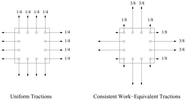
For example, elements with three evenly spaced nodes placed along the face of an element will require loading ratios of ⅙ at the corner nodes and ⅔ at the midpoint node in order to produce a state of uniform stress within the element. Elements with four evenly spaced nodes will require loading ratios of ⅛ at the two corner nodes and ⅜ at the two interior nodes, as illustrated in the right schematic of Fig. 4. These ratios follow from the Lagrange interpolation polynomials used internally by finite elements. They also associate with the weights and quadratures of two well-known integration schemes: Simpson’s rule and Kutta’s ⅜^ths rule, which the author (ADF) has combined into a single, embedded, 4(3) Runge-Kutta method for the numerical integration of non-stiff, ordinary, differential equations (ODEs) [21].

Fig. 4.

The state-of-the-art experimental loading scheme (uniform tractions—the left schematic) versus the proposed loading scheme (consistent work-equivalent tractions from finite-element technology—the right schematic) for inducing a more uniform state of stress within a specimen when subjected to four, discrete, point loads along each edge.

Current, in-plane, biaxial, load frames used to test tissues seek to apply equal tractions at all node-like attachment points along the edges of a specimen [6,7,18], counter to finite-element theory [20]. Theory suggests that the edge loads in the left-hand schematic of Fig. 4 will be too large, and are likely to produce a non-homogeneous state of stress within. Theory also suggests that the loading conditions in the right-hand schematic ought to provide a more homogeneous state of biaxial stress within a test sample.

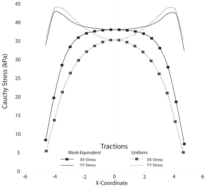
To test this hypothesis, we simulated an equi-force biaxial test of a nearly incompressible neo-Hookean membrane.³ Loads of 180 mN were distributed on a 10 mm × 10 mm, nearly-incompressible membrane 0.5 mm in thickness, having a shear modulus of 50 kPa. The geometry was discretized using an element grid of 25 × 25, linear, plane-stress, membrane elements. Load distributions were those depicted in Fig. 4: uniform tractions, and consistent work-equivalent tractions. Figure 5 plots the Cauchy stress as a function of the horizontal, or X-coordinate. Solid lines correspond to work-equivalent tractions, while dotted lines correspond to uniform tractions. Notably—confirming our hypothesis—the work-equivalent tractions produce a substantially larger region of near-uniform stress, evidenced by the plateau in both the x and y stress components. This difference becomes more marked with increased strain. For a 10 × 10 sample, uniform tractions lead to a ‘sweet area’ for making strain measurements in the middle of the sample of about 2 × 2; whereas, consistent work-equivalent tractions lead to a ‘sweet area’ of about 5 × 5.

Fig. 5.

A finite-element comparison of the loading configurations illustrated in Fig. 4.

The subject of sample conformation and loading has been the topic of previous studies. For example, the idea of using a cruciform as opposed to square samples has been investigated [22]. Our proposition, which holds from first principles, aims to similarly increase the uniformity of stress over an extended area. Furthermore, our approach has the added advantages of being both easier to implement experimentally, and of remaining practical for the smaller samples that are so commonly encountered in biological tissues.

4 Hypoelastic Models

Three, isochoric, hypoelastic, constitutive models were constructed in part I of this paper [1]. The isotropic model is summarized below. Application of the anisotropic and composite models to these data will be the topic of a future paper.

A new, symmetric, strain measure E was also derived in that manuscript. It is described by the ODE

$$\begin{array}{l}D\mathbf{E}=\mathbf{D}+\mathbf{LE}+\mathbf{E}{\mathbf{L}}^T\\ =\mathbf{D}+\mathbf{DE}+\mathbf{ED}+\mathbf{WE}-\mathbf{EW}\text{with}\text{initial}\text{condition}(\text{IC})\mathbf{E}(0)=\mathbf{0},\end{array}$$ (26)

where DE = Ė + ∇E · v is the material derivative of strain that, for the BVP of interest, becomes DE ≃ Ė because, at the center of the tissue being tested, ∇E ≃ 0 over some finite range. The symmetric part of the velocity gradient L is the rate of deformation $\mathbf{D}=\frac{1}{2}(\mathbf{L}+{\mathbf{L}}^T)$, while the skew-symmetric part $\mathbf{W}=\frac{1}{2}(\mathbf{L}-{\mathbf{L}}^T)$ is the spin with W^T = −W [17]. The convected term LE + EL^T, in the sense of Oldroyd, is required in order for E to be a viable tensor field, as established in part I [1]. Alternatively, Eq. (26) can be rewritten as either

$$\partial \mathbf{E}=\mathbf{D}\text{or}\mathring{\mathbf{E}}=\mathbf{D}+\mathbf{DE}+\mathbf{ED},$$ (27)

where ∂E = DE − LE − EL^T defines Oldroyd’s [23] upper-convected, objective, differential operator, and where E˚ = DE − WE + EW defines Jaumann’s [24] objective, differential operator. These are identical descriptions for strain rate, as defined by the author in part I. It was also shown therein that the shear response arising from this differential equation does not oscillate in simple-shear deformations; in fact, $E_{12}=\frac{1}{2}\gamma$ exactly, with no assumptions or restrictions.

The isotropic, isochoric, hypoelastic model derived from a potential function in part I [1] produced the following ODE in Kirchhoff stress

$$D\mathbf{T}+D\wp \mathbf{I}=2(\mu +\alpha \text{tr}\mathbf{T})\widehat{\mathbf{E}}+\beta (\widehat{\mathbf{E}}\mathbf{T}+\mathbf{T}\widehat{\mathbf{E}})+\mathit{\Omega }\mathbf{T}-\mathbf{T}\mathit{\Omega }\text{with}\text{IC}\mathbf{T}(0)=\mathbf{0},$$ (28)

where T̂ = DT − ΩT + TΩ defines the polar rate of stress; it is the objective rate of Green & Naghdi [25]. This rate arises from taking the material derivative DT̄ of stress T̄ residing in a stretched but unrotated frame κ̄ that is then mapped into the spatial frame κ according to the map T̂ = RDT̄R^T [26,27]. In the formula above, D℘ is a Lagrange multiplier forcing an isochoric constraint, tr L = 0. Parameter μ is the small-strain shear modulus, while parameters α and β are analogous to Fung’s coefficient, now expressed in a 3D setting. The polar rate of strain can be written in several forms, depending on how it is to be used, viz.,

$$\begin{array}{l}\widehat{\mathbf{E}}=D\mathbf{E}-\mathit{\Omega }\mathbf{E}+\mathbf{E}\mathit{\Omega }\\ =\mathring{\mathbf{E}}+(\mathbf{W}-\mathit{\Omega })\mathbf{E}-\mathbf{E}(\mathbf{W}-\mathit{\Omega })\\ =\mathbf{D}+\mathbf{DE}+\mathbf{ED}+(\mathbf{W}-\mathit{\Omega })\mathbf{E}-\mathbf{E}(\mathbf{W}-\mathit{\Omega }),\end{array}$$ (29)

where W − Ω is a difference between deformable-body and rigid-body rotation rates [28].

An objective numerical integrator is needed to solve the ODEs given in Eqs. (26 & 28) that characterize this constitutive equation. One such method, a predictor/corrector, is presented in the Appendix.

4.1 Membrane Formulation

The mathematical structure of the evolution (26) and constitutive (28) equations remains unchanged for membranes, except that their tensor fields are now characterized by 2 × 2 matrices, instead of 3 × 3 matrices. What membrane BVPs bring to bear in this construction is a means to solve for the Lagrange multiplier. From the 33-component of this constitutive equation, noting that T_i3 = T_3j = 0 ∀ i, j, because of the plane-stress assumption, one determines that

$$D\wp =2(\mu +\alpha \text{tr}\mathbf{T}){\widehat{E}}_{33}\text{or}\text{equivalently}D\wp =-2(\mu +\alpha \text{tr}\mathbf{T})\frac{\text{tr}\mathbf{D}}{{\mathrm{\Lambda }}^2},$$ (30)

which when combined with Eq. (28) produces

$$D\mathbf{T}=2(\mu +\alpha \text{tr}\mathbf{T})({\mathrm{\Lambda }}^{-2}\text{tr}(\mathbf{D})\mathbf{I}+\widehat{\mathbf{E}})+\beta (\widehat{\mathbf{E}}\mathbf{T}+\mathbf{T}\widehat{\mathbf{E}})+\mathit{\Omega }\mathbf{T}-\mathbf{T}\mathit{\Omega },$$ (31)

as the constitutive equation governing an isotropic, isochoric, hypoelastic membrane of tissue.

To demonstrate that the two equations in expression (30) are equivalent, it suffices to prove that Ê₃₃ = −Λ⁻² trD for the deformation given in Eq. (1). First, from the fact that L₃₃ = D₃₃ = λ̇₃/λ₃, which results from the isochoric constraint put forth in Eq. (2), one can separate variables in the 33-component of Eq. (26), viz., Ė₃₃ = (1 + 2E₃₃)λ̇₃/λ₃, and get its solution $E_{33}=\frac{1}{2}({\lambda }_3^2-1)$. Furthermore, from Eq. (29) and the fact that Ω_i3 = Ω_3j = 0 ∀ i, j, one determines that Ê₃₃ = Ė₃₃ which, using the above result for E₃₃, simplifies to Ė₃₃ = Ê₃₃ = λ₃λ̇₃. The remaining identity λ̇₃/λ₃ = −tr D needed to secure this proof follows from ${\stackrel{.}{\lambda }}_3/{\lambda }_3=-\overline{({\lambda }_1{\lambda }_2-{\gamma }_1{\gamma }_2)}/({\lambda }_1{\lambda }_2-{\gamma }_1{\gamma }_2)=-\stackrel{.}{\mathrm{\Lambda }}/\mathrm{\Lambda }$. To show this, recall that Λ = detF, where F is now given by Eq. (3), not Eq. (2), while noting that detF = det(RU) = det(R) det(U) = detU, recalling that detR = 1, and by making use of the identity d(detU)/dt = det(U)tr(U̇U⁻¹) = det(U)tr[R^T (ḞF⁻¹ − Ω)R] = det(U)tr(ḞF⁻¹) = det(U)tr(L) = det(U)tr(D), and therefore, tr(D) = (detU)⁻¹ d(detU)/dt = Λ̇/Λ = −λ̇₃/λ₃, recalling that Λ = 1/λ₃.

5 Modeling Pericardium

The procedure used to secure the experimental data presented below has been documented in Sun et al. [29]. Small-angle light scattering (SALS) was used to locate a region homogeneous in fiber orientation within a pericardium tissue to be tested, and to determine its dominant fiber direction, which was then aligned with the 1-direction in the author’s (MSS) biaxial test system. The experiments were run in load control at constant rates over like time intervals to targeted values of (protocol; σ₁: σ₂) 1;1:0.1, 2;1:0.3, 3;1:0.5, 4;1:0.75, 5;1:1, 6;0.75:1, 7;0.5:1 and 8;0.1:1, with the listed engineering stresses being in MPa. Only the equi-biaxial experiment (protocol 5 in this test suite) has been published elsewhere [30]. Results from a finite-element analysis done on an existing bioprosthetic heart-valve design was cited by Sellaro et al. [30] as justification for the 10-fold increase in stress imposed upon the specimen in this experiment over the physiologic stresses that were utilized in the earlier study of Billiar & Sacks [19]. Results from that finite-element study found there to be regions near the stent where stresses were an order in magnitude greater than otherwise exist over the belly region.

The raw kinematic data were smoothed using the GCV algorithm and software of Woltring [14], with a cubic B-spline being used to fit the data. An algorithmic regularization parameter that minimizes unbiased estimates of the mean-squared error was selected for filtering and, after a parametric study, was set at 0.0025 for all eight experimental protocols.

5.1 Graphically Obtained Parameter Estimates

It has been the authors’ experience that whenever material parameters can be estimated with reasonable certainty via graphical methods, then they should be so assigned. This helps reduce problems that arise through covariance between parameters during parameter estimation via optimization.

As discussed by the author (ADF) in Ref. [21], isotropic hypoelastic models can discern pressure effects, independent of the Lagrange multiplier, even though the deformation is constrained to be isochoric. Protocols 1, 5 and 8 have loading ratios of 1:0.1, 1:1 and 0.1:1, respectively, and can therefore be used to investigate this pressure effect.

The isotropic hypoelastic solid of Eq. (31) can be solved analytically for the special cases of uniaxial and equi-biaxial extensions. For uniaxial extension, $E_{11}=\frac{1}{2}({\lambda }^2-1),E_{22}=\frac{1}{2}({\lambda }^{-1}-1)$, T₁₁ = τ, and T₂₂ = 0 with stress evolving as

$$\begin{array}{l}\frac{1}{\lambda }\frac{\text{d}\tau }{\text{d}\lambda }=(2+{\lambda }^{-3})\mu +\alpha {\lambda }^{-3}\tau +2(\alpha +\beta )\tau \\ \simeq 3\mu +(3\alpha +2\beta )\tau \end{array}$$ (32)

whereas, for equi-biaxial extension, $E_{11}=E_{22}=\frac{1}{2}({\lambda }^2-1)$, and T₁₁ = T₂₂ = τ with stress evolving as

$$\begin{array}{l}\frac{1}{\lambda }\frac{\text{d}\tau }{\text{d}\lambda }=2(1+2{\lambda }^{-4})\mu +8\alpha {\lambda }^{-4}\tau +2(2\alpha +\beta )\tau \\ \simeq 6\mu +(12\alpha +2\beta )\tau \end{array}$$ (33)

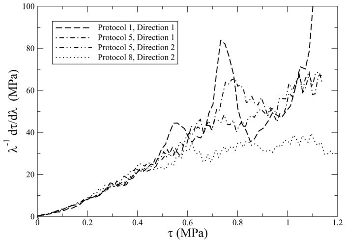
where λ is the stretch, and τ = λσ is the true stress, with these approximations holding in a neighborhood around λ = 1. Although these formulæ do not account for the shear components observed in our experiments, and certain liberties have been imposed regarding the influence of λ, much can still be learned by applying these approximate formulæ to the experimental data of protocols 1, 5 and 8, which is done in Fig. 6. The curves in this figure are analogous to the one originally drawn by Fung [13] for rabbit mesentery, from which he derived the material law that now bears his name.

Fig. 6.

These data are from a glutaraldehyde treated bovine pericardium. Protocols 1 and 8 are approximately uniaxial, while protocol 5 is equi-biaxial. Hypoelasticity predicts that their responses should be straight lines. If there is a pressure effect, accounted for by α, then the uniaxial and equi-biaxial lines will have different slopes; they have the same slope, so α ≈ 0.

The approximate formulæ in Eqs. (32 & 33) are equations for straight lines in a graph of τ vs. λ⁻¹ dτ/dλ. They have different intercepts: 3μ for the uniaxial case, and 6μ for the equi-biaxial case, in accordance with rubber elasticity [31]. They also have different slopes: 3α + 2β for the uniaxial case, and 12α + 2β for the equi-biaxial case. There is minimal scatter in the data up to stresses of about ½ MPa, which is well past the toe/heel region of their stress/strain curves (cf. Figs. 7 & 8). The response is the same for all four curves over this region: linear, except for a small dip near the origin, and they have the same slope. It is in this region that the error of approximation present in Eqs. (32 & 33) is at a minimum, so the conclusions drawn from these data are justified. Based on these data, α ≈ 0 and β ≈ 30, but there is insufficient resolution to estimate μ graphically; however, μ > 0 in order for the stress to integrate away from zero, a typical initial condition. Therefore, Eq. (31) simplifies to

Fig. 7.

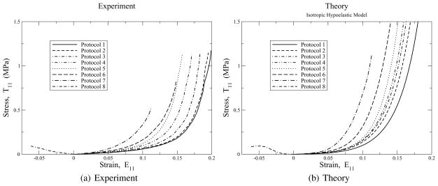
Stress/strain curves in the 1-direction for protocols 1 to 8 imposed on glutaraldehyde treated bovine pericardium. Experimental data are the left figure. Predictions of these data with the isotropic hypoelastic model of Eq. (34) are presented in the right figure. The scales of both figures are the same. Parameters are: μ = 27 kPa and β = 19.2.

Fig. 8.

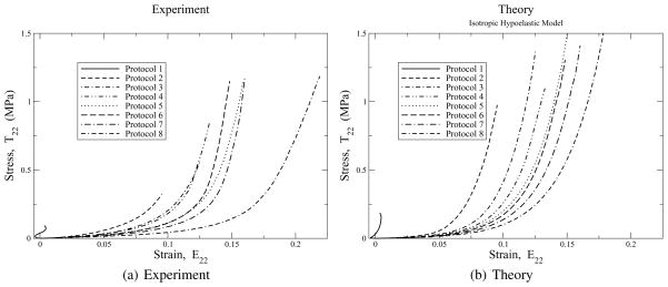
Stress/strain curves in the 2-direction for protocols 1 to 8 imposed on glutaraldehyde treated bovine pericardium. Experimental data are the left figure. Predictions of these data with the isotropic hypoelastic model of Eq. (34) are presented in the right figure. The scales of both figures are the same. Parameters are: μ = 27 kPa and β = 19.2.

$$D\mathbf{T}=2\mu ({\mathrm{\Lambda }}^{-2}\text{tr}(\mathbf{D})\mathbf{I}+\widehat{\mathbf{E}})+\beta (\widehat{\mathbf{E}}\mathbf{T}+\mathbf{T}\widehat{\mathbf{E}})+\mathit{\Omega }\mathbf{T}-\mathbf{T}\mathit{\Omega },$$ (34)

as the isotropic hypoelastic model appropriate for modeling pericardium.

Noise becomes a factor at stresses beyond about ½ MPa. This is in the so-called linear region of the stress/strain response. These data actually suggest that growth remains exponential to stresses exceeding 1 MPa, in an average sense, thereby corroborating Fung’s law, except for protocol 8 which flattens out for stresses in excess of about 0.6 MPa. This appears to be an experimental artifact associated only with protocol 8, based upon a visual inspection of all eight pairs of stress/strain curves presented in Figs. 7(a) and 8(a). Whether this is an experimental anomaly or, for example, a consequence of material anisotropy, is presently unknown.

5.2 Numerically Obtained Parameter Estimates

A genetic algorithm [32,33] was written to maximize a log-likelihood fitness function [34] to estimate parameters μ and β in accordance with the methodology put forward in the Appendix. Only the equi-biaxial experiment, protocol five, was used in the fitting process. The engineering stresses σ₁ and σ₂ were chosen to be the dependent variables of optimization. The 95% confidence intervals for these parameters were determined to be 22.0 < 27.0 < 34.7 for μ (units in kPa) and 18.7 < 19.2 < 19.6 for β, with an R² statistic of 0.909 when derived according to Buse’s [35] formula.

From Fig. 6, Fung’s β parameter was found to be about 30, but from the parameter estimation process, a value of 19.2 was determined as being its most likely value. This disparity is thought to be a byproduct of the over simplified form of the model used. With pericardium being a multi-phased anisotropic tissue, assuming it to be an isotropic continuum requires that its parameters account for more than what they ideally represent. It is expected that the composite model currently under development by the authors will correct this discrepancy.

6 Discussion

Figure 7 contrasts the experimental 7(a) and theoretical 7(b) stress/strain responses in the 1-direction for the eight protocols investigated, which is the dominant fiber direction. The ordering sequence between protocols is correctly predicted by the theory, with the heel spacing being accurately captured, where the heel region is the non-linear part of the stress/strain response separating the fairly linear responses at the two extremes. Actually, the stress/strain response is largely exponential, which is the point of Fig. 6. The theory goes non-linear slightly before what is experimentally observed, which is really its only discernible flaw in this direction. In other words, non-linearity, not anisotropy, is the cause for the translation of the heel region along the strain axis. The modeled response needs improvement in following the stress/strain transition from toe to heel more faithfully. This model is not capable of making that extra improvement. A composite model, with different shear moduli for its matrix and fiber constituents, and the capability of introducing residual stresses, should be able to address this deficiency in a straightforward manner.

Figure 8 contrasts the experimental 8(a) and theoretical 8(b) stress/strain responses in the 2-direction for the eight protocols investigated, which is normal to the fiber dominant direction. A possible influence of anisotropy is manifest in these experimental curves as a retrograde in the sequencing of curves associated with protocols 5 and 6. Then again, this may be due to experimental variability, too. The isotropic model is not capable of describing this experimental observation. However, in the overall scheme of things, this effect is much smaller than that which is due to kinematic non-linearity, which the model seems to capture quite nicely. As in the 1-direction, here too the model goes non-linear at strains earlier than the experiments do. Again, the experimental curve for protocol 8 has a different character about it, whose origin is unknown, and which now becomes more plain when contrasted with its theoretical curve.

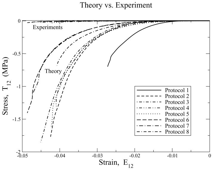
Figure 9 compares the experimental and theoretical stress/strain responses for in-plane shear. Here lies the real Achilles’ heel of this isotropic continuum model. The predicted shear stresses are about two orders in magnitude greater than what are observed experimentally. Least grievous are the uniaxial cases. This is actually not too surprising, as tissue is largely fibrous in composition, and fibers are poorly equipped to handle shears, especially transverse shears. This isotropic model has no machinery in it to allow it to address either transverse shear across the fibers, or longitudinal shear at the fiber/matrix interface, nor can it introduce a softer modulus that controls the shear response of the matrix material binding the fibers together. This model does many things very well, but it is not perfect. Further research is needed to better understand its deficiencies, their physical causes, and how they ought to be accounted for in theory.

Fig. 9.

Shear stress/strain plots for protocols 1 to 8 for glutaraldehyde treated bovine pericardium. Both experimental and theoretical data are plotted, with the experimental data hovering around the zero stress axis. Parameters are: μ =27 kPa and β = 19.2.

It is truly remarkable that any model with only two adjustable parameters can do as-well-as this model has done in describing the very complex, 2D, experimental data considered herein. This lends credence to the conjecture that hypoelasticity is a valid theory for tissues, as speculated by the author (ADF) in Refs. [1, 21, 26].

7 Summary

The paper began with a re-examination of the kinematics of planar biaxial extensions done on membranes. A polar decomposition of the deformation gradient F ensued, leading to stretch and rotation tensors whose components are expressed solely in terms of those belonging to F. When quantifying the kinematic rates, it became necessary to use a smoothing spline to be able to extract meaningful values, as the noise in the data gotten from standard differencing techniques often exceeded the measured signal when estimating the shear components of Ḟ.

For the kinetics of in-plane biaxial experiments containing shear deformations, it has been shown unequivocally that the first Piola-Kirchhoff stress must contain non-zero shear components in order to comply with the conservation of angular momentum. A corrected stress-to-traction mapping has been derived.

A novel scheme for applying tractions to planar specimens has been proposed that should lead to more uniform states of stress within the specimen. This loading mechanism can be applied to small test samples that commonly arise when testing soft tissues.

The isotropic hypoelastic model derived in part I of this manuscript [1] has been altered here for use in membrane analysis. This resulted in a slight restructuring of its constitutive expression in order to account for the influence of the Lagrange multiplier that handles the isochoric constraint.

Non-linear effects are first-order effects in soft tissues that, at least for pericardium, overwhelm the effects caused by strength of anisotropy. Hypoelasticity captures these kinematic non-linearities. Consequently, the simple, isotropic, hypoelastic model, Eq. (34), has a role to play, especially in preliminary analyses. The physical causes behind these non-linearities are varied and many, and whose proper discussion lies well beyond the scope of this paper. It is worthy of note that what one’s eye might associate with as being an anisotropic effect, when viewing an experimental data set for soft tissue, is likely to be a non-linear effect due to kinematics that is in disguise, especially if one’s eye has been trained in the field of small-strain analysis.

Appendix

A Parameter Estimation

Let there be N, experimental, data vectors y_n, n = 1,2,…,N, with components y_n = y(t_n) = {y_n1,y_n2,…,y_nR}^T evaluated at instances t_n, where R is the number of responses or dependent variables that have been measured. From these data, we seek an estimate for K parameters θ = {θ₁,θ₂,…,θ_K}^T that belong to some model (t,θ ) by first creating N residual vectors x_n with components

(35)

that are normalized by their sample standard deviates s̄_r obtained from

$${\overline{s}}_r^2=\frac{1}{N-1}\sum _{n=1}^N{(y_{rn}-{\overline{y}}_r)}^2\text{wherein}{\overline{y}}_r=\frac{1}{N}\sum _{n=1}^N{y}_{rn}.$$ (36)

In the statistical method that follows, x_n are the data, not y_n.

Next, assume that all N data points x_n distribute in accordance with the normal probability density function

$$f({\mathbf{x}}_n)=\frac{1}{{(2\pi )}^{R/2}{(det\mathbf{V})}^{1/2}}exp\left(-\frac{1}{2}{({\mathbf{x}}_n-\mathit{\mu })}^T·{\mathbf{V}}^{-1}({\mathbf{x}}_n-\mathit{\mu })\right),$$ (37)

where vector μ is its mean, and matrix V is its covariance. Finally, assume that these N data points are independent of one another, in which case the likelihood function ℒ becomes the product of its N, probability, density functions

$$\mathcal{L}(\mathit{\theta })={(2\pi )}^{-NR/2}{(det\mathbf{V})}^{-N/2}exp\left(-\frac{1}{2}\sum _{n=1}^N{({\mathbf{x}}_n-\mathit{\mu })}^T·{\mathbf{V}}^{-1}({\mathbf{x}}_n-\mathit{\mu })\right).$$ (38)

Taking the logarithm of both sides gives the well-known result [36]

$$ln(\mathcal{L}(\mathit{\theta }))=-\frac{NR}{2}ln(2\pi )-\frac{N}{2}ln(det\mathbf{V})-\frac{1}{2}\sum _{n=1}^N{({\mathbf{x}}_n-\mathit{\mu })}^T·{\mathbf{V}}^{-1}({\mathbf{x}}_n-\mathit{\mu }),$$ (39)

where μ → 0 and $\frac{1}{2}{\sum }_{n=1}^N{({\mathbf{x}}_n-\mathit{\mu })}^T·{\mathbf{V}}^{-1}({\mathbf{x}}_n-\mathit{\mu })\to NR/2$ in the asymptotic limit where θ goes to its maximum likelihood estimate (MLE) of ϑ. In a neighborhood of this limit, the second term, $\frac{N}{2}ln(det\mathbf{V})$, drives the estimator, and is the cornerstone for classic MLE algorithms [36]. It has been our experience that replacing the third term in (39) with its asymptotic limit can remove valuable information from the optimizer in its search for a MLE.

Instead of replacing the third term in (39) with its asymptotic limit NR/2 and maximizing that expression, maximums for a more complete log-likelihood function are sought; in particular,

$$ln(\mathcal{L}(\mathit{\theta }))=-\frac{NR}{2}ln(2\pi )-\frac{N}{2}ln(det\overline{\mathbf{V}}(\mathit{\theta }))-\frac{1}{2}\sum _{n=1}^N{\mathbf{x}}_n^T(\mathit{\theta })·{\overline{\mathbf{V}}}^{-1}(\mathit{\theta }){\mathbf{x}}_n(\mathit{\theta }),$$ (40)

where the third term adds a generalized least squares component to the otherwise classical likelihood method. Having two competing kernels like this in an objective function does not present a problem when used as a fitness function for a genetic algorithm, as we have done here. In (39), the statistical mean μ has been set to its asymptotic limit of 0, while the variance V has been replaced with its sample variance V̄ whose components are

$${\overline{V}}_{ij}=\frac{1}{N-1}\sum _{n=1}^N(x_{in}-{\overline{x}}_i)(x_{jn}-{\overline{x}}_j)\text{wherein}{\overline{x}}_i=\frac{1}{N}\sum _{n=1}^N{x}_{in}\text{with}i,j=1,2,\dots ,R.$$ (41)

By retaining the sample mean x̄ in the calculation for sample variance V̄, the last term in (40) helps to drive the optimizer towards a solution where the model (t_n,ϑ) becomes a mean to the experimentally measured data y_n, because this term reaches its upper bound of −NR/2 as the model becomes the mean to the data.

B Numerical Integration Method

The ordinary differential equations that present themselves in this theory have the general form

(42)

where Y is the tensor field to be solved for, is some tensor function (it is typically a constitutive equation), and Q is a skew-symmetric operator whose overall effect is to ensure that is an objective differential operator. In our theory, the strain rate employs W for Q (W is the skew-symmetric part of L, with the symmetric part due to D being absorbed into ); whereas, the hypoelastic model employs Ω for Q. There are many other objective rates in use in the literature [37,38] that utilize other definitions for Q.

To establish a numerical scheme for integrating (42), it is insightful to first rewrite this differential equation as an equivalent integral equation, and to express it at two sequential instances, say at n and n + 1, such that

(43)

(44)

wherein

$$\mathbf{G}={\mathbf{F}}_{n+1}{\mathbf{F}}_n^{-1}={\mathbf{F}}_{t_{n+1}}^1(t_n)$$ (45)

is a push-forward operator that maps tensor fields from configuration κ_n into κ_n+1, and is some function of .

To be able to solve the integral in the second line of (44), some integrators may require one to evaluate Ẏ_n in κ_n+1, which we denote as (Ẏ_n)_n+1, while Ẏ_n+1 in κ_n+1 is gotten straightaway from (42). To determine (Ẏ_n)_n+1, operate on both sides of Eq. (44) with the derivative ∂/∂t_n, such that after rearranging and gathering terms, one gets

(46)

This rate resides in κ_n+1, because the equation from which it was derived, Eq. (44), resides within κ_n+1. To arrive at the convective terms in the above equation requires one know ∂G/∂t_n. From the identity $\partial {\mathbf{F}}_n{\mathbf{F}}_n^{-1}/\partial t_n=\partial \mathbf{I}/\partial t_n=\mathbf{0}$, one determines that $\partial {\mathbf{F}}_n^{-1}/\partial t_n=-{\mathbf{F}}_n^{-1}{\mathbf{L}}_n$, so that $\partial \mathbf{G}/\partial t_n={\mathbf{F}}_{n+1}\partial {\mathbf{F}}_n^{-1}/\partial t_n=-\mathbf{G}{\mathbf{L}}_n$. This result generalizes for other objective rates where L_n can be replaced by an admissible Q_n in the last two terms.

A second-order, predictor/corrector, integration algorithm developed for the above integral equation follows.

Interface

Input: h, F_n−1, F_n, F_n+1, L_n, L_n+1, Q_n, Q_n+1, Y_n−1, Y_n and function and for heterogeneous BVPs: v_n, v_n+1 and ∇Y_n

Output: Y_n+1

Map

$$\begin{array}{l}{\mathbf{G}}_{n-1}={\mathbf{F}}_n{\mathbf{F}}_{n-1}^{-1}\\ {\mathbf{G}}_n={\mathbf{F}}_{n+1}{\mathbf{F}}_n^{-1}\end{array}$$

Predictor: midpoint integration in κ_n, where h = t_n+1 −t_n ∀ n, n = 0,1,…,N − 1

Push the required tensors forward from κ_n into κ_n+1

$$\begin{array}{l}{({\mathbf{Y}}_n)}_{n+1}={\mathbf{G}}_n{\mathbf{Y}}_n{\mathbf{G}}_n^T\\ {(\nabla {\mathbf{Y}}_n)}_{n+1}={\mathbf{G}}_n(\nabla {\mathbf{Y}}_n){\mathbf{G}}_n^T·{\mathbf{G}}_n^{-1}\\ {\mathbf{Y}}_p={\mathbf{G}}_n{({\mathbf{Y}}_p)}_n{\mathbf{G}}_n^T\end{array}$$

Corrector: trapezoidal integration in κ_n+1

These formulæ simplify for homogeneous deformation histories, like occur in most experimental BVPs done on solids, in that the spatial gradients ∇Y · v are zero valued there, or at least negligible. One can use forward Euler integration, viz., (Y_p)₀ = Y₀ + hẎ₀, to start this integrator.

At each summation configuration along the solution path, all sums of integration are done within that configuration, in accordance with our prior discussion [1]. The solution progresses along a path of configurations with a ratcheting motion of push-forward/summing operations that progresses over the entire loading history.

We have taken liberties here by replacing ∇Y_p · v_n+1 with ${(\nabla {\mathbf{Y}}_n)}_{n+1}·{\mathbf{v}}_{n+1}={\mathbf{G}}_n(\nabla {\mathbf{Y}}_n){\mathbf{G}}_n^T·{\mathbf{G}}_n^{-1}{\mathbf{v}}_{n+1}$ in the second line of the corrector in order to keep this a one-pass procedure. The first operator G_n pushes the left component of Y_n into κ_n+1. The second operator ${\mathbf{G}}_n^T$ maps the right component of Y_n. While the third operator ${\mathbf{G}}_n^{-1}$ converts ∇_n into ∇_n+1. In other words, we have pushed the gradient ∇Y_n forward into configuration κ_n+1 in place of using ∇Y_p, whose use would otherwise require that the algorithm become implicit in its spatial variables.

References

- 1.Freed AD. Hypoelastic Soft Tissues, Part I: theory. Acta Mechanica 2010 doi: 10.1007/s00707-010-0357-y. ??? [DOI] [PMC free article] [PubMed] [Google Scholar]
- 2.Hwang NHC, Nan XZ, Gross DR. Prosthetic heart valve replacements. Critical Reviews in Biomedical Engineering. 1982;9:99–132. [PubMed] [Google Scholar]
- 3.Vesely I. New concepts in the design and use of biological prosthetic valves. Cardiovascular Pathology. 1995;4:287–291. doi: 10.1016/1054-8807(95)00055-a. [DOI] [PubMed] [Google Scholar]
- 4.Sacks MS, Chuong CJ. Orthotropic mechanical properties of chemically treated bovine pericardium. Annals of Biomedical Engineering. 1998;26:892–902. doi: 10.1114/1.135. [DOI] [PubMed] [Google Scholar]
- 5.Sacks MS, Sun W. Multiaxial mechanical behavior of biological materials. Annual Review of Biomedical Engineering. 2003;5:251–284. doi: 10.1146/annurev.bioeng.5.011303.120714. [DOI] [PubMed] [Google Scholar]
- 6.Sacks MS. Biaxial mechanical evaluation of planar biological materials. Journal of Elasticity. 2000;61:199–246. [Google Scholar]
- 7.Humphrey JD. Cardiovascular Solid Mechanics; cells, tissues, and organs. Springer-Verlag; New York: 2002. [Google Scholar]
- 8.Holzapfel GA, Ogden RW. On planar biaxial tests for anisotropic nonlinearly elastic solids. A continuum mechanical framework. Mathematics and Mechanics of Solids. 2009;14:474–489. [Google Scholar]
- 9.Dokos S, Smaill BH, Young AA, LeGrice IJ. Shear properties of passive ventricular myocardium. American Journal of Physiology–Heart and Circulatory Physiology. 2002;283:H2650–H2659. doi: 10.1152/ajpheart.00111.2002. [DOI] [PubMed] [Google Scholar]
- 10.Sacks MS. A method for planar biaxial mechanical testing that includes in-plane shear. Journal of Biomechanical Engineering. 1999;121:551–555. doi: 10.1115/1.2835086. [DOI] [PubMed] [Google Scholar]
- 11.Hoffman AH, Grigg P. A method for measuring strains in soft tissue. Journal of Biomechanics. 1984;17:795–800. doi: 10.1016/0021-9290(84)90110-6. [DOI] [PubMed] [Google Scholar]
- 12.Humphrey JD, Vawter DL, Vito RP. Quantification of strains in biaxially tested soft tissues. Journal of Biomechanics. 1987;20:59–65. doi: 10.1016/0021-9290(87)90267-3. [DOI] [PubMed] [Google Scholar]
- 13.Fung YC. Elasticity of soft tissues in simple elongation. American Journal of Physiology. 1967;28:1532–1544. doi: 10.1152/ajplegacy.1967.213.6.1532. [DOI] [PubMed] [Google Scholar]
- 14.Woltring HJ. A FORTRAN package for generalized, cross-validatory spline smoothing and differentiation. Advances in Engineering Software. 1986;8:104–113. [Google Scholar]
- 15.Silverman BW. Some aspects of the spline smoothing approach to non-parametric regression curve fitting. Journal of the Royal Statistical Society, B. 1985;47:1–52. [Google Scholar]
- 16.Ogden RW. Non-Linear Elastic Deformations. John Wiley; New York: 1984. republished by Dover Publications, Mineola, NY, 1997. [Google Scholar]
- 17.Holzapfel GA. Nonlinear Solid Mechanics: A continuum approach for engineering. Wiley; Chichester: 2000. [Google Scholar]
- 18.Fung YC. Biomechanics: mechanical properties of living tissues. 2. Springer-Verlag; New York: 1993. [Google Scholar]
- 19.Billiar KL, Sacks MS. Biaxial mechanical properties of the natural and glutaraldehyde treated aortic valve cusp–part I: experimental results. Journal of Biomechanical Engineering. 2000;122:23–30. doi: 10.1115/1.429624. [DOI] [PubMed] [Google Scholar]
- 20.Cook RD, Malkus DS, Plesha ME, Witt RJ. Concepts and Applications of Finite Element Analysis. 4. Wiley; New York: 2002. [Google Scholar]
- 21.Freed AD. Anisotropy in hypoelastic soft-tissue mechanics, II: simple extensional experiments. Journal of Mechanics of Materials and Structures. 2009;4(6):1005–1025. [Google Scholar]
- 22.Waldman SD, Lee JM. Effect of sample geometry on the apparent biaxial mechanical behaviour of planar connective tissues. Biomaterials. 2005;26:7504–7513. doi: 10.1016/j.biomaterials.2005.05.056. [DOI] [PubMed] [Google Scholar]
- 23.Oldroyd JG. On the formulation of rheological equations of state. Proceedings of the Royal Society, London, A. 1950;200:523–541. [Google Scholar]
- 24.Jaumann G. Geschlossenes System physikalischer und chemischer Differential gesetze. Sitzungsberichte der Kaiserlichen Akademie der Wissenschaften: Mathematisch-naturwissenschaftliche Klasse. 1911;120:385–530. [Google Scholar]
- 25.Green AE, Naghdi PM. A general theory of an elastic-plastic continuum. Archives for Rational Mechanics and Analysis. 1965;18:251–281. [Google Scholar]
- 26.Freed AD. Anisotropy in hypoelastic soft-tissue mechanics, I: theory. Journal of Mechanics of Materials and Structures. 2008;3(5):911–928. [Google Scholar]
- 27.Dienes JK. On the analysis of rotation and stress rate in deforming bodies. Acta Mechanica. 1979;32:217–232. [Google Scholar]
- 28.Dienes JK. A discussion of material rotation and stress rate. Acta Mechanica. 1986;65:1–11. [Google Scholar]
- 29.Sun W, Sacks MS, Fulchiero G, Lovekamp J, Vyavahare N, Scott M. Response of heterograft heart valve biomaterials to moderate cyclic loading. Journal of Biomedical Materials Research. 2004;69A:658–669. doi: 10.1002/jbm.a.30031. [DOI] [PubMed] [Google Scholar]
- 30.Sellaro TL, Hildebrand D, Lu Q, Vyavahare N, Scott M, Sacks MS. Effects of collagen fiber orientation on the response of biologically derived soft tissue biomaterials to cyclic loading. Journal of Biomedical Materials Research. 2007;80A:194–205. doi: 10.1002/jbm.a.30871. [DOI] [PubMed] [Google Scholar]
- 31.Treloar LRG. The Physics of Rubber Elasticity. 3. Clarendon Press; Oxford: 1975. [Google Scholar]
- 32.Goldberg DE. Genetic Algorithms in Search, Optimization, and Machine Learning. Addison-Wesley; Boston: 1989. [Google Scholar]
- 33.Goldberg DE. Genetic Algorithms and Evolutionary Computation. Vol. 7. Kluwer; Boston: 2002. The Design of Innovation: Lessons learned from and for Competent Genetic Algorithms. [Google Scholar]
- 34.Sharman KC, McClurkin GD. Genetic algorithms for maximum likelihood parameter estimation. 1989 International Conference on Acoustics, Speech and Signal Processing; Glosgow, Scotland: IEEE; 1989. pp. 2716–2719. [Google Scholar]
- 35.Buse A. Goodness of fit in generalized least squares estimation. American Statistician. 1973;27:106–108. [Google Scholar]
- 36.Bard Y. Nonlinear Parameter Estimation. Academic Press; New York: 1974. [Google Scholar]
- 37.Meyers A, Schieße P, Bruhns OT. Some comments on objective rates of symmetric Eulerian tensors with applications to Eulerian strain rates. Acta Mechanica. 2000;139:91–103. [Google Scholar]
- 38.Szabó L, Balla M. Comparison of some stress rates. International Journal of Solids and Structures. 1989;25:279–297. [Google Scholar]