Abstract
Graphical analysis (GA) is an efficient method for estimating total tissue distribution volume (VT) from positron emission tomography (PET) uptake data. The original GA produces a negative bias in VT in the presence of noise. Estimates of VT using other GA forms have less bias but less precision. Here, we show how the bias terms are related between the GA methods and how using an instrumental variable (IV) can also reduce bias. Results are based on simulations of a two-compartment model with VT's ranging from 10.5 to 64 mL/cm3 and from PET image data with the tracer [11C]DASB ([11C]-3-amino-4-(2-dimethylaminomethyl-phenylsulfanyl) benzonitrile). Four estimates of VT (or distribution volume ratio (DVR) using a reference tissue) can be easily computed from different formulations of GA including the IV. As noise affects the estimates from all four differently, they generally do not provide the same estimates. By taking the median value of the four estimates, we can decrease the bias and reduce the effect of large values contributing to noisy images. The variance of the four estimates can serve as a guide to the reliability of the median estimate. This may provide a general method for the generation of parametric images with little bias and good precision.
Keywords: distribution volume, distribution volume ratio, graphical analysis, instrumental variable, modeling, positron emission tomography
Introduction
Positron emission tomography (PET) provides images of the distribution time course of radiotracers in tissue. Physiological information can be extracted from this data by the application of compartment models using an arterial plasma input function that consists of the concentration (radioactivity) of the tracer versus time. The direct application of compartment models requires a nonlinear estimation technique to obtain the kinetic parameters associated with the model (Carson, 1980). Patlak et al (1983) introduced a transformation of the compartmental equations for irreversible systems such that ordinary least squares could be applied to the transformed equations to obtain a physiological measure designated as the influx constant, which is a composite of the model parameters. This technique is referred to as graphical analysis (GA). An extension to reversibly binding tracers provides an estimate of the total tissue distribution volume (VT) (Logan et al, 1990). As most PET radiotracers bind reversibly, the latter technique has been used more extensively. Graphical analysis has important advantages, it is simple to implement and does not require that a particular model structure be adopted for the analysis, which makes it desirable for use in voxel wise image analysis. However, the original version used for reversible radiotracers suffers from a noise-dependent bias, which results in the underestimation of the distribution volume (Carson, 1993; Slifstein and Laruelle, 2000).
The utility of the GA approach has led to a number of papers suggesting modifications to reduce the bias. Varga and Szabo (2002) proposed the total least squares estimation referred to as the ‘perpendicular linear regression model' however, this only partially removes the bias. Ichise et al (2002) proposed a rearrangement of the GA equation (referred to as MA1) that resulted in reduced bias. Ogden (2003) introduced the likelihood estimation in graphical analysis (LEGA) method for estimating the parameters in the linear portion of the GA equation. This involves estimation through an iterative minimization process using a recursive relation for radiotracer concentration and its numerical integral in the GA equation. An improvement on LEGA that reduced the variance of VT using a maximum a posteriori-based estimation was introduced by Shidahara et al (2009). The approach taken by Joshi et al (2008) is a principal component analysis that is applied to image data before the analysis step. This reduces the noise and increases precision compared with other noise removal processes but requires the preprocessing step, which must be optimized with respect to the number of principal components used. However, too many principal components reintroduces the bias. The most recent contribution to this literature is Zhou et al (2009), who propose using the plasma radioactivity in the denominator of the GA plot. This was also extended to a reference tissue (RT) method. This, however, requires that the tissue to plasma ratio be constant, limiting the application to certain tracers. Ito et al (2010) introduced an unrelated graphic method specific for a two-compartment model, which provided unbiased estimates of VT but the estimates are subject to variation with noise.
In this paper, we compare several arrangements of the GA equation as well as an instrumental variable (IV) method for reducing bias in least squares estimation. The IV approach was introduced by Young (1970) and Stoica and Soderstrom (1983). Minchin (1978) applied the IV approach of Young to tracer experiments of phloem translocation in plants. We tested the IV method using the iterative approach used by Minchin as well as an alternative method in which the IV is constructed from a smooth time–activity curve (TAC). These methods were applied to simulations of a two-tissue compartment model, with total distribution volumes ranging from 10.5 to 64 (mL/cm3) and to voxel image data from PET studies with the serotonin transporter tracer [11C]DASB ([11C]-3-amino-4-(2-dimethylaminomethyl-phenylsulfanyl) benzonitrile).
Theoretical Background
Formulations of the Graphical Analysis Method
The original equation for the graphical analysis of reversible PET radiotracers is given in equation (1a) (designated GA)
 |
where ROI(t) is the radioactivity in tissue at time t after injection and Cp(t) is the plasma radioactivity corrected for the presence of labeled metabolites at time t (Logan et al, 1990). For some time after injection, that is for t>t* a plot of equation (1a) becomes linear with slope β1, the total tissue distribution volume, VT. β2, the intercept, is a function of model parameters. A noise-dependent bias results in the underestimation of the distribution volume β1. If the tissue radioactivity measure at time t contains noise, there is an error term at each time point. Writing equation (1a) in terms of the ‘true' parameter vector  , an error term at time tn (where n designates a particular time frame), ɛ(n), can be defined in equation (1b) as (Soderstrom and Stoica, 2002)
 |
In the absence of noise ɛ(n) is zero. Rewriting equation (1a) in a matrix form gives
where YT=[y(k)…y(N)] and ΘT=[ϑT(k)…ϑT(N)], with k being the index of t* (at which linearity is observed) and N the index of the last frame. The components of Y and Θ are given by  ,
,  , 1] respectively, and the error is E=Y−Θ
 where ET=[ɛ(k)…ɛ(N)].
The vectors β and  are
are 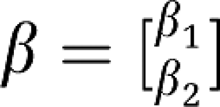 and
and 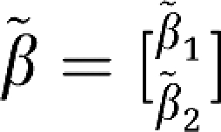 .
.
The estimation error in β, becomes (Soderstrom and Stoica, 2002)
 |
where
and
β is unbiased if the second term on the right-hand side is zero.
Equation (1a) can be rearranged into an alternative form shown in equation (3a) (designated GA1),
 |
Equation (1b) can be rearranged to give the error term for GA1 in terms of the error term for GA
 |
Therefore, the magnitude of the bias error term for GA1 is reduced compared with that for GA (equation (1b) if  1>1. Converting equation (1c) to a bilinear form where
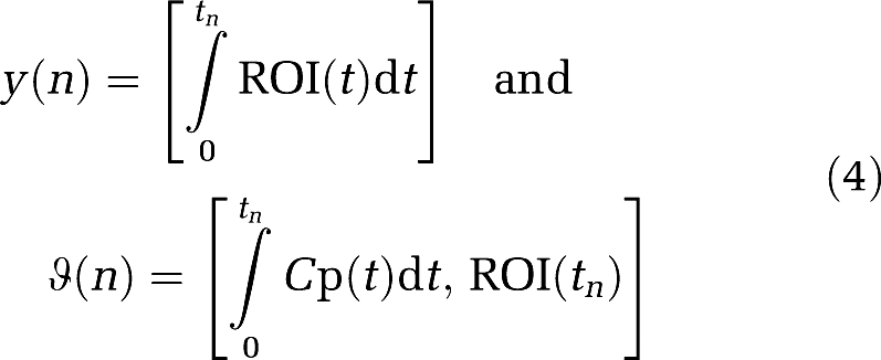 |
gives
 |
Using  1 and
1 and  2 as the true values, the bias error term equation (5b) is
 |
Equations (5a) and (5b) can be rearranged into equations (6a) and (6b)
 |
 |
so that the magnitude of the bias for Equation (6a) is less than that of equation (5a) if  1>1. The ROI(tn) term does not contribute to the bias error in the estimation of β in equations (5b) and (6b), that is β−
 =(ΘTΘ)−1ΘTE is the same if the elements of E are replaced by E(tn)ROI(tn) and the elements of Θ are defined as in equation (4).
The bilinear version MA1 (Ichise et al, 2002) is given by
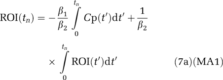 |
with
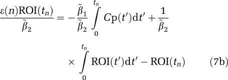 |
Therefore, the magnitude of the bias in the estimation of β using equation (7a) would be expected to be less than that using equation (6a) if ∣ 2∣>∣
2∣>∣ 1∣ and less than equation (5a) for ∣
 2∣>1. We will use simulations to investigate the influence of the error term on the estimation of β1 for these different formulations of GA.
Instrumental Variable
An alternative method for reducing bias is the use of an IV. The IV methods have been used to eliminate the bias in the estimation of parameters from a set of linear algebraic equations when the independent variable contains noise as it does in the GA equations, particularly equation (1a). The degree of bias is dependent upon the noise/signal ratio (Young, 1970).
The IV method is an extension of the least squares method. Starting with the general equation in matrix form including the noise term E (Soderstrom and Stoica, 2002).
we can solve for β in a manner similar to the least squares method using an IV  ,
,
 |
If  T and E are independent and the distribution of E is mean zero the expected value of the last term is zero and the estimation of β (Young, 1970) is
 |
.
When  =Θ equations (9) and (10) reduce to the normal equations. The problem lies in determining the IV. It is necessary that the inverse matrix in equation (10) be nonsingular, that the true value for β be recovered from equation (10) using
  (t) when Y(t) and Θ(t) are noise free and that IV be uncorrelated with E (or that (
 TΘ)−1
TΘ)−1 TE → 0). Two alternative methods for constructing an IV for the GA of PET data are considered. For the first case an iterative method is used for generating an IV. This has been proposed by Minchin (1978) based on the work of Young (1970). The steps adapted to the GA problem for generating
  are:
are:
(1) Make an initial estimate of the parameters β1 and β2 using the GA formulation (the other forms have less bias and do not need the IV intervention).
(2) Use β1 and β2 to generate estimated values of  (n), designated
  (n) (by estimating values of ROI(tn)). For example,
  (n) from equation (1c) becomes
 |
where Z*(t) is the estimated ROI(t) evaluated using the recursion relation developed by Ogden (equation (12) below) and the estimated vector β. Y remains the same.
(3) Using  (with elements
  (n)) as the IV a new estimate of β is obtained.
This can be repeated until β converges.
The recursion formula introduced by (Ogden, 2003) relates the estimated ROI(ti) designated Zi*
 |
to Zi−1* where ti is the midpoint of scan i, si is the end point of scan i, and (si−si−1) is the length of scan i. This relationship is derived from equation (1a) by using the trapezoidal rule for the integral of the scan from the beginning of i to the midpoint at ti where the integral from 0 to the end of scan i−1 (which corresponds to si−1), is
 |
For times before the linear part measured ROI values are used.
A second method for the IV is much simpler to apply and does not require multiple determinations as in the iterative method described above. For this we propose to use a ‘noise-free' TAC generated from a region of interest with sufficient voxels that the curve is smooth to form  . In addition to requiring that (
 TΘ)−1
TΘ)−1 TE → 0, the IV must also produce the ‘true' value of β1 when Θ and Y are the noise-free ‘true' data. This is obviously achieved when
  is formed from the ‘true' noise-free data. As this will usually not be available, another potential choice for a TAC with which to construct
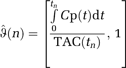
  would be to use the reference region or a global region. In this case, the IV components of
  are
are
 |
Both of these IV methods were tested with simulations described below.
Extension to Reference Tissue (RT) Analysis
The extension of equation (1a) to a RT model is given by (Logan et al, 1996)
 |
Substituting for Cp(t)
 |
where Ψ1 is the distribution volume ratio (DVR) of the region of interest to the reference tissue (REF). (The DVR is related to the nondisplaceable-binding potential, BPND, as DVR=1+BPND.) β2=−(1/k2), k2 is the tissue to plasma efflux constant for the RT, taken to be a population average. An alternative version (Ichise and Ballinger, 1996) is
 |
which allows the determination of k2 directly from Ψ′2. Equations (12) and (13) can be rearranged into alternative forms based on those using plasma input. Corresponding to equation (3a)
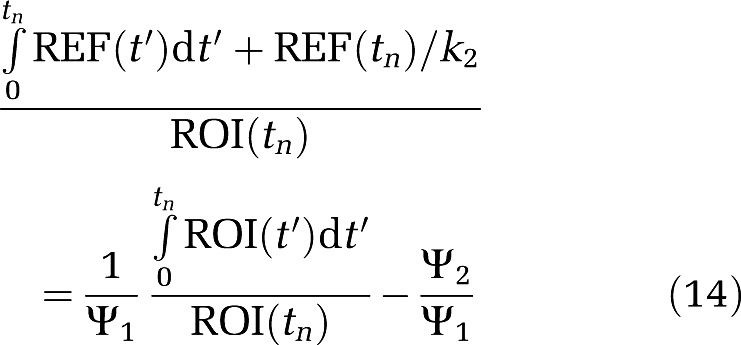 |
and from equation (8a) (Ichise et al, 2003), MRTM2
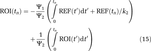 |
The strategy (Ichise et al, 2003) is to evaluate k2 from equation (13) using regions of interest from the RT and from a receptor region that contain a sufficient number of voxels that noise is not an important factor. This value can then be used in linear models of equations (12), (14), and (15).
The IV methods can also be applied to the RT equations to remove bias. For equation (12), (DVR(GA)) the  (n) are given by
 |
Materials and methods
Generation of Simulated Data
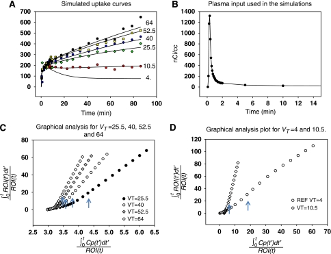
A two-compartment model was used to generate the simulation data. Model parameters K1=0.35 mL/min/cm3 and k2=0.086 min−1 were used for the transfer constants between blood and tissue (and to generate data simulating RT). The value for k4 was fixed (k4=0.0475 min−1) and five values of k3 (0.075, 0.25, 0.42, 0.565 and 0.7 min−1) were used giving for β1 (VT) 10.5, 25.5, 40.05, 52.5 and 64.05 mL/cm3 respectively. (The units for VT are always mL/cm3.) Corresponding values for β2 are −42.88, −90.52, −133.4, −169.4 and −202.7 (min) (  ). The scanning protocol consisted of 24 frames: 4 (30 seconds), 8 (1 minute), 4 (5 minutes), 8 (7.5 minutes) for a total of 90 minutes. Uptake curves for this data are shown in Figure 1A. The solid lines represent the noise-free data and the symbols correspond to examples from each noisy data set. A measured plasma input function was used (injected dose 7.1 mCi) (Figure 1B). Gaussian noise was added to each error-free simulated time frame (
  ) as
) as  where
where
Figure 1.
(A) Simulated uptake data for six values of the total distribution volume. The ‘reference region' VT=4 is based on a one-compartment model using only K1 and k2. The other curves are two-compartment model simulations with k4=0.0475 min−1 and k3 values of 0.075, 0.25, 0.42. 0.565, and 0.7 min−1 corresponding to VT=10.5, 25.5, 40, 52.5, and 64 mL/cm3, respectively. The solid lines are the noise-free data, and the symbols correspond to selected time–activity curves (TACs) with noise. (B) Plasma input used in the simulations was taken from a human study with 7.1 mCi injected dose. Only the first 15 minutes are shown but the input function extends to 100 minutes. (C) Plots of graphical analysis (GA) using equation (1a) for VT=25.5, 40, 52.5, and 64. In all cases, linearity was achieved by 22 minutes indicated with arrows. (D) Plots of GA using equation (1a) for VT=4 mL/cm3 (reference tissue) and VT=10.5 mL/cm3. VT, total tissue distribution volume.
 |
SD is the standard deviation approximation for decay-corrected radioactivity counts (Vesa Oikonen Turku PET Centre Modelling report TPCMOD0008 2003-01-19). G(0,1) is a pseudo-random number from a Gaussian distribution generated in IDL (http://www.ittvis.com/idl). The decay constant of the isotope (11C with a half-life of 20.4 minutes) is λ. At each noise level, 1000 data sets were generated for each example. Only one value of Sc (Sc=1) was used to set the noise level. However, as the VT was varied from 10.5 to 64 mL/cm3, the effects of noise while small for VT=10.5 were much greater for 52.5 and 64.5 mL/cm3.
Times for the linear portion were taken to be between 22 and 90 minutes. Plots of the GA using equation (1a) for the noise-free simulated data are shown in Figures 1C and 1D.
The four versions of the graphical analysis equation, equations (1a) and (3a) and the bilinear versions, equations (5a) and (6a) and MA1 (equation (7a)) as well as the IV methods were used to test the effect of noise on the estimation of the total distribution volume, β1. For the noniterative IV method, three different TACs were used: (1) a noise-free version of the data set being tested, (2) a noise-free RT ROI, and (3) as a test, an ROI formed by placing 1's for each time point in the ROI. All of these functions returned the true value of β1 when noise-free data were used. Results are only reported for the RT ROI as in a practical situation the true noise-free data would not be known.
Besides the mean, s.d. and bias, results are presented in terms of box plots and distributions (SigmaPlot 9) of parameter estimates from selected simulations. For each box in a box plot, the upper and lower edges are determined by the 75th and 25th percentile of the data and the line in between is the median. The error bars indicate 90th and 10th percentile. The open or closed circles indicate values at 95th and 5th percentile. For the distribution plots, the histogram function of SigmaPlot 9 was used within a user-defined function transform.
Application to Image Data
Image data from five studies with the serotonin transporter ligand, [11C]DASB, synthesized according to the method developed by Wilson et al (2000) were used. The PET data were acquired over a 90-minute period using a whole body, high-resolution positron emission tomograph (Siemen's HR+ 4.5 × 4.5 × 4.8 mm3 at the center of field of view) in 3D dynamic acquisition mode. An arterial plasma input function for [11C]DASB was obtained, samples were drawn every 2.5 seconds for the first 2 minutes (Ole Dich automatic blood sampler), then at 3, 4, 5, 6, 8, 10, 15, 20, 30, 45, 60, and up to 90 minutes. All samples were centrifuged to obtain plasma and selected samples are assayed for the presence of unchanged [11C]DASB. The average injected dose was 8.71±0.32 mCi. The scanning protocol (number of scans and scan length) was 3 × 20 seconds, 3 × 1 minute, 3 × 2 minutes, 2 × 5 minutes, and 7 × 10 minutes. Voxels for analysis were selected from three adjacent planes containing maximum uptake as determined by the integrated radioactivity over 90 minutes. Voxels of low, intermediate, and high uptake were separated based on the value of the integrated image (maximum=100). Voxels of low uptake were taken as those between 22% and 25% of the maximum. Intermediate values were 40% to 42.5% and high values were 80% to 100%. The analyses were performed on each voxel within the group, and the VT estimates averaged over all voxels in each group were compared with the VT estimated from the ROI formed using all voxels. Because of the high noise level in individual voxels, it is necessary to have a scheme for minimizing the effect of outliers. To do this, we defined a maximum value so that if any estimated VT exceeded that value it was eliminated before forming the median. In the DASB calculations, the maximum value was set to 100 (two times the maximum ROI value for these data sets). Negative values were also eliminated. However, a number of outliers remained. If the voxel noise level is great, the VT estimates will differ considerably. We hypothesized that if the variance of the estimates exceeds a certain value, none of them will be reliable. This was validated by comparing VT estimates of the DASB data that exhibited high variance to the estimates of lower variance.
Proposed Method
The estimation of VT (or DVR) using the four methods GA, GA1, MA1, and IV (GA with IV using a smooth TAC for the IV) does not present a computational burden in parametric image generation, as these are all linear equations. These estimations generally provide different values because of the different effect of noise in the formulation of each one. We have tried to define a simple procedure for increasing the precision of the VT estimate for images. The methods GA1, MA1, and IV all have less bias than GA equation (1a) but are subject to outliers (values that can be considerably larger than the true value) with increasing noise. To reduce the effect of these outliers and obtain reliable estimates of VT, we propose to take the median value of the four estimates as the best estimate of the VT. This eliminates the highest and lowest value and uses the average of the middle two. In some cases, the median may be formed by fewer estimates if one was eliminated by exceeding a preset threshold. In the presence of low noise, the four estimates should be fairly close with a low variance. With increasing noise, the variance of the estimates for each voxel increases. By defining a maximum allowed variance those voxels can be identified for which accurate estimates cannot be obtained. In such cases, some smoothing (i.e., combining voxels or clustering) can be performed.
Results
Error in Estimate of β1 for the Five Forms of Graphical Analysis
In Table 1, the difference of β1− 1 averaged over all data sets for each value of VT are given for methods GA, GA1, MA1, GAbi, and GA1bi. The first entry is the mean of β1−
 1 for that value of VT (
 1=true VT value). The average difference β1−
 1 for GA and GAbi are very close as is the average for GA1 and GA1bi. The method MA1 has the least bias of all GA forms. The entries in parentheses are the averages over all data sets of the error terms summed over all time points included in the linear estimation. For each data set, the error term for GA is the sum of ɛ(n)
Table 1. Bias and ERR for five arrangements of the graphical analysis equation.
| VT | GA | GA1 | GAbi | GA1bi | MA1 |
|---|---|---|---|---|---|
| 10.5 | −0.57 (0.098) | −0.39 (0.0094) | −0.51 (466) | −0.30 (42) | −0.02 (10.9) |
| 25.5 | −2.74 (5.2) | −1.09 (0.2) | −2.9 (754) | −0.92 (29.5) | 0.31 (8.3) |
| 40 | −6.8 (0.384) | −1.7 (0.0096) | −7.5 (1100) | −1.4 (27.5) | 1.6 (8.25) |
| 52.5 | −12.1 (1.7) | −2.16 (0.032) | −13.6 (874) | −1.6 (16.6) | 4.2 (5.2) |
| 64 | −18.5 (2.5) | −2.24 (0.039) | −20.9 (771.5) | −0.91 (12.05) | 14.8 (3.81) |
VT, total tissue distribution volume.
The first entry is the error term for β1 (VT) calculated for the five graphical analysis methods as the average (β1− 1) over all data sets (N=1000) for each VT value.
  1 is the ‘true' value and β1 is the value estimated from the individual data set. The number in parentheses refers to the error term (ERR) calculated as equations (17) and (18) for GA and GA1. The extension to the other forms uses the absolute value of the sum of time points for equations (5b), (6b), and (7b) averaged over all data sets. For each VT (
 ) value, ERR for GA1 is equal to the value for ERR(GA)/VT and also ERR(biGA1)=ERR(GAbi)/
 1 while ERR(MA1)=ERR(GAbi)/∣
 2∣.
2∣.
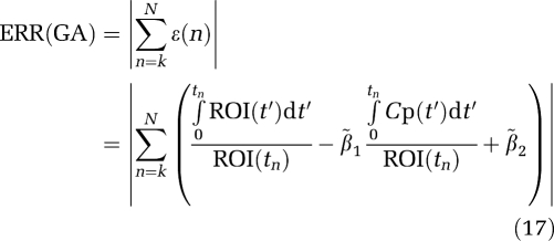 |
and for GA1
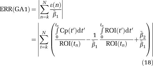 |
Similarly the error terms for GAbi, GA1bi, and MA1 can be found by summing ɛ(n) in equations (5b), (6b), and (7b), respectively. From Table 1, the error for GA1 is less than GA for VT=40, ERR(GA) is 0.384 and for GA1 it is 0.384/40=0.0096 and similarly for VT=52.5 the ratio 1.7/52.5=0.032 gives ERR (GA1). Therefore, the bias in the estimation of β1 is less for GA1 than for GA in all examples. The error terms for the bilinear formulations are larger than those for GA and GA1 because of the presence of ROI(t) in equations (6b), (7b), and (8b). From Table 1, the error for MA1 which is 5.2 for VT=52.5 is related to that of GAbi as 874/169.4=5.2. The biases for GA and GAbi (and GA1 and GA1bi) are essentially the same. Of the bilinear forms MA1 has the smallest error of all three and the least bias for the lowest VT values but is subject to large outliers with increasing noise so that for these simulations the average of β1− 1 becomes larger for the higher values of β1. Apparently, the presence of the ROI term while not contributing to bias contributes to loss of precision because of an increase in the number of independent variables compared with GA (Shidahara et al, 2009).
Comparison of Simulation Results for Graphical Analysis Using the Five Equation Forms and the Instrumental Variable Calculations of VT
Table 2 presents the mean±s.d. (percent bias) for VT over all data sets using the methods, GA, GA1, GAbi GA1bi, and MA1 as well as the two IV methods and the median. (In this table, bias is reported as percent of the true value.) Consistent with the results in Table 1, the mean for VT is less biased for GA1 and GA1bi than for GA or GAbi. The method MA1 is the least biased but produces more outliers (defined here as values >100) for the higher VT values. For VT=64, MA1 produced 100 values >100. The GA1bi produced the second most outliers (50 values >100 for VT=64). The method MA1 has the largest s.d. and is the estimation method with the least precision. For VT=52.5 and 64, results are reported using all data and replacing values >100 with the GA value. For VT=64, that last entry in the median column eliminates VT estimates with variances >400 (99/1000). This reduces the average to 59.8 but the s.d. is also less so that the coefficient of variation is the same as for the GA estimates. The differences between the methods are less for the smaller values of VT (a result of the using the same noise scale factor for all simulations) for VT=10.5, the bias is −5% for GA and ∼−4% for GA1. For VT=40, this becomes −20% for GA and −5% for GA1.
Table 2. Mean±s.d. (% bias) for VT (mL/cm3) for all data sets (N=1000) for five graphical analysis methods and two IV methods and the median.
| VT | GA | GA1 | GAbi | GA1bi | MA1 | IV (Iterative) | IV (TAC=REF) | Median of (GA, GA1, MA1, IVRT) |
|---|---|---|---|---|---|---|---|---|
| 10.5 | 9.93±0.66 (−5.4) | 10.1±0.70 (−3.7) | 9.99±0.64 (−5) | 10.20±0.64 (−2.8) | 10.5±0.79 (0.2) | 10.40±0.75 (−0.95) | 10.4±0.7 (−1) | 10.24±0.7 (−2.4) |
| 25.5 | 22.8±2.4 (−10.7) | 24.4±2.9 (−4.2) | 22.6±2.5 (−11) | 24.6±3.2 (−3.6) | 25.8±3.79 (1.3) | 25.5±3.2 (−0.17) | 25.4±3 (−0.3) | 24.8±3.0 (−2.6) |
| 40 | 32.9±4.5 (−20) | 38.3±6.2 (−4.3) | 32.2±4.6 (−19) | 38.3±6.6 (−4.2) | 41.6±9.9 (4) | 40.3±7.0 (1.0) | 40.4±6.9 (1) | 39.0±6.5 (−2.3) |
| 52.5 | 40.4±6.5 (−23) | 50.3±11 (−4) | 38.8±7 (−26) | 50.9±13.6 (−3) | 56.6±23 (8) | 53.6±14.5 (3) | 53.9±13 (2.8) | 51.5±11 (−2) |
| 52.5 | 50.0±11 (−4) | 53±12 (1) | 53.6±13 (2) | 53.2±11.3 (1.3) | 49.5±8.5 (−3) | |||
| 64 | 45.6±8.3 (−28) | 61.8±18 (−2.7) | 43.3±9.3 (−32) | 62±22 (−3) | 70.7±29.8 (10) | 66.5±18 (4) | 65.±15.2 (1.8) | 62.7±16 (−2.4) |
| 64 | 59.8±12.5 (−6.5) | 59.4±13.8 (−7.1) | 61.5±14.9 (−3.9) | 63.5±14.4 (−0.7) | 62.3±12.7 (−2) | 60.1±12 (−5) | ||
| 64 | 59.8±10.6 (−6.5)a |
IV, instrumental variable; TAC, time–activity curve; VT, total tissue distribution volume; REF, reference tissue.
The second entry for VT=52.5 and 64 replaces values >100 with the GA value. The IV methods use the GA formulation. The column labeled IV (TAC=ref) refers to results using the reference tissue for TAC in  (t) in equation (13). The last column is the median of the four values where IV refers to the method using TAC.
Uses median filtering to eliminate median estimates in which the variance exceeded 400.
Results using the iterative IV method are given in column labeled IV (iterative). There is a general reduction in bias with an increase in s.d. compared with GA. The coefficient of variation (s.d./mean) is 0.17 for VT=40 and 0.12 for VT=25.5. There were very few outliers found for the lower VT values. For VT=64, however, the number of outliers was greater. Although calculations were performed for all three of the TACs described previously, results are reported for TAC using RT for TAC in the GA form, equation (13). There was little difference in results using the other two TACs; however, ROI1 produced a few more outliers. The IV calculated with the smooth TAC's was found to be preferred over the iterative method as only one calculation was involved (although the iterative method generally requires only a few interations) and also because it was more stable. The iterative method failed for a number of voxels particularly in conditions of high noise.
According to Young (1970), the IV reduces bias in the parameter estimate by virtue of the fact that it is uncorrelated with the error. However, with the use of TACs other than the ‘true ROI' to form the IV, this condition will not necessarily hold. Comparing the first element of the vector  TE with ΘTE, where E=Y−Θ
 and
and
the average of  TE is −69 compared with −26.9 (average using simulated data sets for VT=52.5). However, we also find that
 |
(N is the number of simulated data sets and i is the index for each data set). This inequality gives 1.45 for left side of equation (19) versus 12.8 for the right side. The condition for the IV to remove bias is then that ( TΘi)−1
 T is uncorrelated with E.
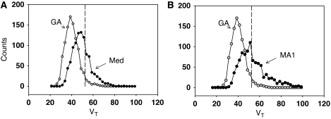
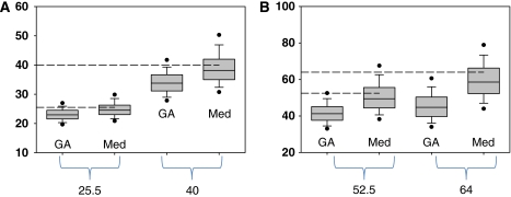
The last column in Table 2 reports the average (over all data sets) of the median value of GA, GA1, MA1, and IV. There is a small bias of 5% to 6% at the highest value. Figure 2A is a plot of the distribution of the VT estimates for VT=52.5 using GA (equation (1a)) and of the median of the four estimates for VT=52.5 (N=1000). There is less bias for the median than for GA; however, the distribution for the median is broader. Figure 2B compares the same GA distribution for VT=52.5 mL/cm3 with that of the MA1 estimates. There is a substantial number of values in the tail of the distribution such that 17% of the estimated values are >20% above the true value. Although less than MA1, distribution plots of methods GA1 and IV (not shown) also exhibit a significant number of values in this region. Figure 3 presents box plots of VT of the median and of GA estimates for VT=25.5 and 40 (Figure 3A) and VT=52.5 and 64 (Figure 3B). The spread in values is somewhat larger for the median than for GA and the presence of a greater number of large values is indicated by the 5% and 95% circles. For all values of VT, the median represents less bias with an increase in spread of values. For VT=64, the median value with the variance filtering (eliminating ∼10% of the values) was used, which reduced the spread in VT estimates from that of the unfiltered median. The presence of a larger spread of values will contribute to image noise.
Figure 2.
(A) Histogram plot (bin size 2.5 VT units) illustrating the distribution of VT estimates for GA and the median value for VT=52.5 mL/cm3 (dashed line). In all, 3% of estimated values were above 67.4, which is 20% above the true value. (B) Histogram plot illustrating the distribution of VT estimates for GA and MA1 for VT=52.5 (same bin size as A). In all, 17% of estimated values were above 67.4% or 20% above the true value. VT, total tissue distribution volume.
Figure 3.
Box plots comparing GA and the median (Med) of the four estimates for VT=25.5 and 40 mL/cm3 (A) and) VT=52.5 and 64 mL/cm3. (B). For VT=64, the median value with the variance filtering was used (this eliminates about 10% of the values, reducing the spread in estimates). The ‘true' values are indicated with dashed lines. VT, total tissue distribution volume.
Comparison of Simulation Results for Distribution Volume Ratio Determined by Graphical Analysis
The DVR calculations corresponding to equations (12), (14), and (15), designated DVR(GA), DVR(GA1), and MRTM2 for the five data sets are given in Table 3. Here, it was assumed that an accurate k2 was previously calculated from the noise-free ROI according to equation (13). The IV calculation using the RT to form  in equation (16) is also reported. The MRTM2 generated a few values outside the realm of possibility, some <0 and some >100. These values were set to the corresponding DVR(GA) for the statistics given in Table 3 under MRTM2 for the first entry for 12.89 and 15.74. The second entry for 12.89 and 15.74 in Table 3 replaces values >30 with the DVR(GA) value. The first entry for GA1 under 15.74 was without filtering. No filtering was performed on the other estimations. The DVR estimation using MRTM2 was unbiased after the filtering described but with greater variability than the other methods. The median is given in the last column and is less biased than DVR(GA) and has less variability than any one individual method except GA.
Table 3. DVR for GA, GA1, MRTM2, IV, and the median as mean±s.d. (% bias).
| DVR | GA | GA1 | MRTM2 | IV | Median (GA, GA1, MA1, IV) |
|---|---|---|---|---|---|
| 2.58 | 2.43±0.16 (−5.7) | 2.48±0.17 (−3.8) | 2.57±0.19 (−0.3) | 2.55±0.18 (−1) | 2.50±0.17 (−3.1) |
| 6.26 | 5.58±0.6 (−10.8) | 5.99±0.7 (−4.4) | 6.33±0.93 (1.1) | 6.28±0.94 (0.4) | 6.09±0.77 (−2.8) |
| 9.84 | 8.15±1.1 (−17) | 9.39±1.6 (−4.5) | 10.2±2.4 (3.7) | 10.05±2.3 (2.5) | 9.61±1.8 (−2.3) |
| 12.89 | 9.47±1.7 (−26) | 12.36±3.4 (−4.2) | 14.2±6.4 (10.6) | 13.2±3.1 (2.5) | 12.5±2.2 (−3) |
| 12.89 | 12.15±3.3 (−6) | 13.1±3 (2.1) | |||
| 15.74 | 11.2±2.0 (−29) | 15.1±4.2 (−4) | 17.4±7.4 (10) | 16.5±5.2 (4.6) | 15.5±4.2 (−1) |
| 15.74 | 14.9±3.6 (−5.4) | 15.9±4.5 (1.0) | 15.9±3.9 (0.8) | 15.2±3.6 (−3) |
DVR, distribution volume ratio; IV, instrumental variable; TAC, time–activity curve.
The IV calculation used the GA form (equation (12)) with Θ (t) defined as in equation (16) with reference tissue as TAC. In the second entries for 12.895 and 15.74 values of MRTM2>30 were replaced with the GA value.
Comparison of Results for Alternative Forms of Graphical Analysis Using Image Data from Studies with the Positron Emission Tomography Ligand [11C]DASB
Results from the four graphical methods applied to [11C]DASB data are reported in Table 4. The last column (ROI) is the VT estimated using the voxel average at each time point to generate a ‘ROI'. As this involves a fairly large number of voxels, this is taken to be the ‘true' value for comparison. For columns labeled GA, GA1, GAIV, and MA1, the VT estimates are performed for each voxel and the results are averaged. The VT values <0 were eliminated from the statistical computations. These were only a few. The total numbers of voxels are given in parentheses in column GA. Results in column 7 (median) are given as the median and the median for which voxels with a variance >50 were excluded. In two cases, there were a significant number of voxels with variances exceeding 50, study 603BH (particularly Med) and study 516BH. The average percent bias over all five studies for GA was −12.4±4.9, −6.3±4.7, and −3.57±3.8 for low, intermediate, (Med) and high uptake, respectively. Using the median (with the variance filter) gave biases of 0.97±0.57, 1.57±0.96, and 0.50±3.0 for low, intermediate, and high uptake, respectively. The greatest bias and the greatest variance in the graphical estimates occurred for the lowest VT estimates, most likely related to the lower counts and therefore greater noise.
Table 4. Comparison of GA, GA1, GAIV, MA1, and median VT values (mean±s.d.) (no. of voxels) averaged over voxels selected from three planes of five DASB dynamic images.
| Study | Uptake | GA | GA1 | IV | MA1 | Median | ROI |
|---|---|---|---|---|---|---|---|
| 280DH (9.0 mCi) | Low | 6.7±1.42 (733) | 7.03±1.82 | 7.37±2.08 | 7.50±2.21 | 7.17±1.86 (733) | 7.2 |
| Med | 10.2±1.82 (2133) | 10.3±2.26 | 10.5±2.51 | 10.5±2.68 | 10.4±2.19 (2129) | 10.5 | |
| High | 26.8±2.31 (183) | 27.0±2.53 | 27.2±2.53 | 27.3±2.60 | 27.1±2.48 (183) | 28.0 | |
| 491AH (8.81 mCi) | Low | 6.70±1.42 (555) | 7.23±1.82 | 7.64±2.35 | 7.90±4.64 | 7.38±1.95 (553) | 7.45 |
| Med | 12.2±1.87 (1244) | 12.6±2.43 | 13.0±2.88 | 13.1±3.36 | 12.7±2.4 (1244) | 12.9 | |
| High | 31.9±4.95 (528) | 32.3±5.26 | 32.7±5.42 | 32.7±5.51 | 32.5±5.3 (528) | 32.7 | |
| 603CH (8.51 mCi) | Low | 4.50±0.95 (525) | 5.28±2.55 | 6.24±4.63 | 6.82±13.3 | 5.59±2.91 (525) | 5.32 |
| 5.25±1.62 (507)* | |||||||
| Med | 8.43±1.95 (749) | 11.1±9.6 | 13.7±22 | 14.2±26 | 10.9±6.50 (748) | 9.84 | |
| 9.57±2.89 (690)* | |||||||
| High | 25.6±4.83 (638) | 27.9±7.3 | 29.1±8.5 | 29.2±8.2 | 28.3±7.6 (638) | 27.45 | |
| 27.3±5.74 (603)* | |||||||
| 513CH (9.11 mCi) | Low | 7.28±1.71 (963) | 9.37±5.25 | 10.8±9.2 | 10.8±8.8 | 9.74±5.28 (963) | 8.84 |
| 8.80±2.75 (895)* | |||||||
| Med | 11.2±1.75 (1548) | 11.6±2.66 | 12.1±3.20 | 12.1±2.74 | 11.8±2.72 (1548) | 11.8 | |
| 11.7±2.33 (1536)* | |||||||
| High | 30.6±4.22 (133) | 31.1±4.50 | 31.5±4.54 | 31.5±4.49 | 31.2±4.49 (133) | 29.9 | |
| 516BH(8.25 mCi) | Low | 9.91±2.65 (894) | 12.8±8.1 | 16.5±44 | 16.0±31 | 13.0±7.7 (894) | 11.5 |
| 11.3±3.43 (819)* | |||||||
| Med | 17.7±4.06 (1196) | 19.2±7.5 | 20.2±9.1 | 20.5±11.0 | 19.54±7.7 (1194) | 18.3 | |
| 18.4±4.5 (1147)* | |||||||
| High | 46.5±4.66 (327) | 47.7±5.3 | 48.3±5.54 | 48.3±5.6 | 47.8±5.2 (327) | 48.9 |
DASB, 3-amino-4-(2-dimethylaminomethyl-phenylsulfanyl) benzonitrile; IV, instrumental variable; ROI, region of interest; VT, total tissue distribution volume.
Voxels in the low uptake category corresponded to the fraction of the integrated image that ranged from 22% to 25% of the maximum, the intermediate category (Med) corresponded to between 40% and 42.5%, and the high was 80% to 100%. The numbers of voxels used in the average are given in parentheses. For the median calculation, average estimates labeled with * were calculated by excluding voxels for which the variance was >50. The last column is the VT calculated from the average over all voxels.
Data from studies 516BH and 603CH were used to test whether the variance of the four graphical estimates represents a good measure of noise and therefore reliability of the median. After eliminating estimates <0 and >100, the average of estimates for which the variance exceeded 50 were 8.99±4.36 (GA), 32.9±17 (GA1), 40±16 (IV), and 42.7±24 (MA1) compared with the ROI value of 11.5 (516BH low). The GA estimates were closest but biased. Restricting the average to estimates with variance <10 gave 9.9±2.16 (GA), 10.6±2.89 (GA1), 11.2±3.2 (IV), and 11.3±3.1 (MA1), which compare more favorably to the ROI value. For study 603CH, the average VT estimates with variances exceeding 50 were 8.1±3.4 (GA), 29.1±13.7 (GA1), 38.7±13.8 (IV), 42.9±19.4 (MA1) compared with the ROI value 9.84. For variances <10, the averages were 8.38±1.72 (GA), 8.97±2.37 (GA1), 9.57±2.69 (IV), and 9.75±2.72 (MA1). We conclude that the variance of the individual estimates is a reasonable way to determine if the noise level is too high to give a good estimate of VT using graphical methods.
Discussion
The construction of PET brain images of receptor binding is complicated by noise at the voxel level as well as the large number of voxels in an image. The nonlinear estimation techniques used for estimating the kinetic constants associated with a compartment model are not appropriate for use in image-wide analysis. If the data conform to a one-compartment model and a RT exists, the simplified RT models can be used (Gunn et al, 1997; Wu and Carson, 2002). However, in many cases, these conditions are not met or only partially met if the data does not quite conform to a one-compartment model. An alternative and more general method is graphical analysis that transforms the differential equations of compartmental analysis into a least squares form that gives the VT without having to specify a particular model structure. This is an advantage when working with images as the model may change in moving from one region of an image to another. There are a number of versions of the graphical analysis equation. Using a measured plasma input function these versions are GA (equation (1)), GA1 (equation (4a)), GAbi (equation (6a)), GA1bi (equation (7a)), and MA1 (equation (8a)). We have compared the bias and precision effects of the estimations of VT for simulated data sets as well as image voxel data for low, intermediate, and high uptake. As a constant noise factor was used in the simulations, the simulations with higher VT had greater noise and bias in the GA estimate, whereas the image data did well at the high VT levels and more poorly at the low values because of the lower count rate.
Using the simulation data, we have shown that the bias in the estimation of VT is related to the error terms defined in equations (17) and (18) for GA and GA1 and by summing over the time points in equations (5b), (6b), and (7b) for MA1, GAbi, and GA1bi. The negative bias in GA is substantially removed by rearrangements GA1 and GA1bi (as  1>1) and for MA1 (as ∣
 2∣>1) The bias for GA1 ∼4% to 6% for all VTs and for MA1 it is even less for the smaller VTs. For GA, the bias increased with VT from 11% for VT=25.5% to 30% for VT=64. Similar results were found for the RT methods.
We have shown that IV methods also reduce bias. Using simulation data, the iterative method of Minchin that we adapted to PET data using the recursive relation given by Ogden produced estimates with much less bias than GA. However, it is an iterative process somewhat time consuming and more prone to outliers than using a noise-free TAC, which we found gave the same results. It made no difference if this was the ‘true' TAC from which the simulated data was derived or the TAC representing a ‘reference' tissue. The IV method reported in Table 2 appeared to perform better than MA1 in that the bias was substantially removed with less loss of precision. A reasonable choice for a TAC to use in forming the IV is either a RT or a global TAC, which includes a large number of voxels from the image. It appears that the condition for the success in the IV method using the TACs other than the ‘true' TAC is due to equation (19) rather than that the IV itself is uncorrelated with the noise vector.
The reduction in bias of these alternative graphical methods comes with a price, and that is loss of precision compared with GA. This problem is common to other methods proposed for reducing bias and results in noisy parametric images (Joshi et al, 2008). The loss of precision is related to the noise level. In the actual image data in Table 4, loss of precision occurred for the lower uptake voxels, particularly for studies 603CH and 516BH. The presence of these large values can be the source of significant image noise as seen in Joshi et al (2008) and will affect image quantitation. The variance of the four graphical estimates appears to provide a useful way to identify whether the median estimate of VT is reliable. Alternative measure can be taken when this is found to be the case. In such cases, a clustering of local voxels can be used or the GA value can be substituted, although it tends to be biased, it is less likely to contribute a large value to the image. Alternatively a principal component analysis could be applied.
In summary, there are essentially four graphical type methods related to equation (1a) that provide estimates of VT with somewhat different biases and precision. These are GA, GA1, MA1, and IV, the methods labeled GAbi and GA1bi were not included as they produce essentially the same bias as GA and GA1. The estimation of VT (or DVR using DVR(GA), DVR(GA1), MRTM2, and DVR(IV)) using all four methods is not computationally expensive as they are all linear methods. As they all provide estimates of VT but with different sensitivities to noise, we propose that the best estimate may be to take the median value of the four estimates. It may first be necessary to remove or replace any values that are outside a specified expected range as MA1 in particular can generate some unrealistic values. Using a variance filter on the median, most outliers can be identified for further processing. The proposed method offers a possibility of balancing the bias versus precision effects in the generation of parametric images.
The authors declare no conflict of interest.
Footnotes
This study was performed at Brookhaven National Laboratory under contract DE-AC02-98CH10886.
References
- Carson R.1980Parameter estimation in positron emission tomography Positron Emission Tomography and Autoradiography: Principles and Applications for Brain and Heart(Phelps ME, Mazziotta J, Schelbert H, eds)New York: Raven Press; 347–390. [Google Scholar]
- Carson R.1993PET parameter estimation using linear integration methods: bias and variability consideration Quantification of Brain Function: Tracer Kinetics and Image Analysis in Brain PET(Uemura K, Lassen NA, Jones T et al (eds))Amsterdam: Elsevier Science Publishers B.V.499–507. [Google Scholar]
- Gunn R, Lammertsma A, Hume S, Cunningham V. Parametric imaging of ligand-receptor binding in PET using a simplified reference region model. Neuroimage. 1997;6:279–287. doi: 10.1006/nimg.1997.0303. [DOI] [PubMed] [Google Scholar]
- Ichise M, Ballinger J. From graphical analysis to multilinear regression analysis of reversible radioligand binding. J Cereb Blood Flow Metab. 1996;16:750–752. doi: 10.1097/00004647-199607000-00028. [DOI] [PubMed] [Google Scholar]
- Ichise M, Liow JS, Lu JQ, Takano T, Model K, Toyama H, Suhara T, Suzuki T, Innis RB, Carson TE. Linearized reference tissue parametric imaging methods: application to C-11 DASB positron emission tomography studies of the serotonin transporter in human brain. J Cereb Blood Flow Metab. 2003;23:1096–1112. doi: 10.1097/01.WCB.0000085441.37552.CA. [DOI] [PubMed] [Google Scholar]
- Ichise M, Toyama H, Innis R, Carson R. Strategies to improve neuroreceptor parameter estimation by linear regression analysis. J Cereb Blood Flow Metab. 2002;22:1271–1281. doi: 10.1097/01.WCB.0000038000.34930.4E. [DOI] [PubMed] [Google Scholar]
- Ito H, Yokoi T, Ikoma Y, Shidahara M, Seki C, Naganawa M, Takahashi H, Takano H, Kimura Y, Ichise M, Suhara T. A new graphic plot analysis for determination of neuroreceptor binding in positron emission tomography studies. Neuroimage. 2010;49:578–586. doi: 10.1016/j.neuroimage.2009.07.021. [DOI] [PubMed] [Google Scholar]
- Joshi AD, Fessler JA, Koeppe RA. Improving PET receptor binding estimates from Logan plots using principal component analysis. J Cereb Blood Flow Metab. 2008;28:852–865. doi: 10.1038/sj.jcbfm.9600584. [DOI] [PMC free article] [PubMed] [Google Scholar]
- Logan J, Fowler J, Volkow N, Wang G, Ding Y, Alexoff D. Distribution volume ratios without blood sampling from graphical analysis of PET data. J Cereb Blood Flow Metab. 1996;16:834–840. doi: 10.1097/00004647-199609000-00008. [DOI] [PubMed] [Google Scholar]
- Logan J, Fowler J, Volkow N, Wolf A, Dewey S, Schlyer D, MacGregor R, Hitzemann R, Bendriem B, Gatley S. Graphical analysis of reversible radioligand binding from time-activity measurements applied to [N-11C-methyl]-(−)-cocaine PET studies in human subjects. J Cereb Blood Flow Metab. 1990;10:740–747. doi: 10.1038/jcbfm.1990.127. [DOI] [PubMed] [Google Scholar]
- Minchin PEH. Analysis of tracer profiles with applications to phloem transport. J Exp Bot. 1978;29:1441–1450. [Google Scholar]
- Ogden R. Estimation of kinetic parameters in graphical analysis of PET imaging data. Stat Med. 2003;22:3557–3568. doi: 10.1002/sim.1562. [DOI] [PubMed] [Google Scholar]
- Patlak C, Blasberg R, Fenstermacher J. Graphical evaluation of blood-to-brain transfer constants from multiple-time uptake data. J Cereb Blood Flow Metab. 1983;3:1–7. doi: 10.1038/jcbfm.1983.1. [DOI] [PubMed] [Google Scholar]
- Shidahara M, Seki C, Naganawa M, Sakata M, Ishikawa M, Ito H, Kanno I, Ishiwata K, Kimura Y. Improvement of likelihood estimation in Logan graphical analysis using maximum a posteriori for neuroreceptor PET imaging. J Cereb Blood Flow Metab. 2009;23:163–171. doi: 10.1007/s12149-008-0226-0. [DOI] [PubMed] [Google Scholar]
- Slifstein M, Laruelle M. Effects of statistical noise on graphic analysis of PET neuroreceptor studies. J Nuclear Med. 2000;41:2083–2088. [PubMed] [Google Scholar]
- Soderstrom T, Stoica P. Instrumental variable methods for system identification. Circuits Syst Signal Process. 2002;21:1–9. [Google Scholar]
- Stoica P, Soderstrom T. Optimal instrumental variable estimation and approximate implementations. IEEE Trans Automat Control. 1983;28:757–772. [Google Scholar]
- Varga J, Szabo Z. Modified regression model for the Logan plot. J Cereb Blood Flow Metab. 2002;22:240–244. doi: 10.1097/00004647-200202000-00012. [DOI] [PMC free article] [PubMed] [Google Scholar]
- Wilson AA, Ginovart N, Schmidt M, Meyer JH. Novel radiotracers for imaging the serotonin transporter by positron emission tomography: synthesis, radio synthesis, and in vitro and ex vivo evaluation of 11C-labeled 2-(Phenylthio)araalkylamines. J Med Chem. 2000;43:3103–3110. doi: 10.1021/jm000079i. [DOI] [PubMed] [Google Scholar]
- Wu Y, Carson R. Noise reduction in the simplified reference tissue model for neuroreceptor functional imaging. J Cereb Blood Flow Metab. 2002;22:1440–1452. doi: 10.1097/01.WCB.0000033967.83623.34. [DOI] [PubMed] [Google Scholar]
- Young P. An instrumental variable method for real-time identification of a noisy process. Automatica. 1970;6:271–287. [Google Scholar]
- Zhou Y, Ye WG, Brasic JR, Crabb AH, Hilton J, Wong DF. A consistent and efficient graphical analysis method to improve the quantification of reversible tracer binding in radioligand receptor dynamic PET studies. Neuroimage. 2009;44:661–670. doi: 10.1016/j.neuroimage.2008.09.021. [DOI] [PMC free article] [PubMed] [Google Scholar]


