Semi-supervised Pattern Classification of Medical Images: Application to Mild Cognitive Impairment (MCI)

Abstract

Many progressive disorders are characterized by unclear or transient diagnoses for specific subgroups of patients. Commonly used supervised pattern recognition methodology may not be the most suitable approach to deriving image-based biomarkers in such cases, as it relies on the availability of categorically labeled data (e.g., patients and controls). In this paper, we explore the potential of semi-supervised pattern classification to provide image-based biomarkers in the absence of precise diagnostic information for some individuals. We employ semi-supervised support vector machines (SVM) and apply them to the problem of classifying MR brain images of patients with uncertain diagnoses. We examine patterns in serial scans of ADNI participants with mild cognitive impairment (MCI), and propose that in the absence of sufficient follow-up evaluations of individuals with MCI, semi-supervised strategy is potentially more appropriate than the fully-supervised paradigm employed up to date.

1. Introduction

High-dimensional pattern classification has gained significant attention in recent years, and has been found to be a promising technique for capturing complex spatial patterns of pathological brain changes (Davatzikos et al., 2009; Fan et al., 2008c; Vemuri et al., 2009; McEvoy et al., 2009; Hinrichs et al., 2009; Duchesne et al., 2008b; Kloppel et al., 2008). Importantly, pattern classification methods have begun to provide tests of high sensitivity and specificity on an individual patient basis, in addition to characterizing group differences. As the result, these methods can potentially be used as diagnostic and prognostic tools. Pattern classification approaches were shown to work particularly well in the task of classifying patient populations from normal cohort in various clinical studies (e.g., Alzheimer’s (Duchesne et al., 2008a; Fan et al., 2008a; Kloppel et al., 2008; Misra et al., 2009), autism (Ecker et al., 2010), schizophrenia (Fan et al., 2008b), etc.).

The state-of-the-art brain image classification methods work by learning a classification function from a set of labeled training examples, and then apply the learned classifier to predict labels of the test data. These methods belong to the family of supervised classification approaches and assume that the labels for all training data are available. Depending on the machine learning method applied, there are many different classification functions that separate a given pair of classes. Support vector machines (SVM) have been shown to provide high classification accuracy, and are among the most widely used classification algorithms in the brain MRI classification literature (Fan et al., 2008a; Kloppel et al., 2008; Misra et al., 2009; Ecker et al., 2010; Fan et al., 2008b). However, many disorders, especially progressive ones, are characterized by uncertain or transient diagnoses for specific subgroups of patients. For example, one might be interested in classifying subjects with mild cognitive impairment (MCI) into classes that either exhibit or do not exhibit future convergence to Alzheimer’s disease (AD). Unfortunately, many subjects are likely to have insufficient follow-up studies to be called converters or non-converters with high confidence. Training a supervised classifier in the scenarios where diagnoses (i.e., labels) are uncertain or unavailable may not be appropriate. Semi-supervised classification approaches are specifically designed to handle cases where only part of the data is labeled. These approaches simultaneously use both labeled and unlabeled data to infer a classifier that provides good classification of the unlabeled data into the two classes.

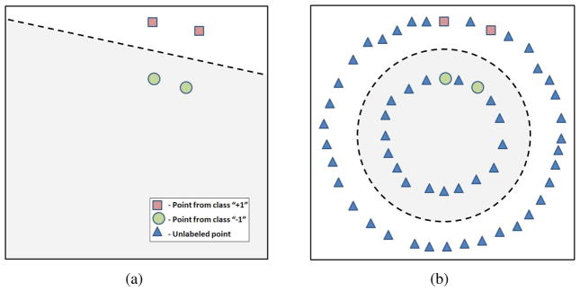
Semi-supervised SVM (Vapnik, 1998) extend the theory of traditional SVM to the case of partially labeled datasets, and offer both the accuracy of traditional SVM, and the ability to use unlabeled data to learn more reliable classification functions. Additionally, semi-supervised SVM have been shown to be more efficient than the traditional SVM in problems with a small number of labeled examples (Joachims, 1999). One of the reasons why semi-supervised SVM learning can benefit from unlabeled data is that unlabeled data can help the classifier better learn the structure of the manifold on which image samples lie. A schematic example of one of the benefits that consideration of unlabeled data provides is depicted in Figure 1. While a fully-supervised classifier can be constructed to separate labeled points as in Figure 1(a), it fails to generalize well if the actual distribution is more complex than the distribution of the labeled instances (i.e., Figure 1(b)). In contrast, semi-supervised SVM considers both labeled and unlabeled data, and may be more appropriate in the scenario where the labeled population does not entirely reflect the structure of the data.

Figure 1.

Benefits of semi-supervised SVM. (a) Fully supervised classifier (represented by a dashed line) does not consider unlabeled data, and separates only the labeled points. (b) Semi-supervised classifier (represented by a dashed circle) considers unlabeled data points, and may have a better generalization ability.

The application focus of this paper is on Alzheimer’s Disease (AD). The incidence of Alzheimers disease (AD) doubles every 5 years after the age of 65, rendering the disease the major cause for dementia, as well as a very important health and socioecomic issue, particularly in view of increasing life expectancy (Bain et al., 2008; Hebert et al., 2001). Although most currently approved treatments are symptomatic and do not directly slow AD pathology progression, it is anticipated that new disease modifying treatments will be available in the near future. It is also expected that treatment decisions will greatly benefit from diagnostic and prognostic tools that identify individuals likely to progress to dementia sooner. This is especially important in individuals with mild cognitive impairment (MCI), who present a conversion rate of approximately 15% per year.

The task of predicting short term conversion to AD from MCI has been addressed in the past with the help of fully supervised techniques that aim at deducing a decision function from a set of labeled images (e.g., normal control, AD, MCI-Converters, etc.) (Duchesne et al., 2008a; Fan et al., 2008a; Kloppel et al., 2008; Misra et al., 2009). However populations of individuals with MCI are highly heterogeneous. Previous studies suggest that some MCIs are close to AD and will convert soon, whereas some will remain stable for over a decade. Moreover, while some individuals with MCI may convert at a faster rate than others to AD, some will never develop AD and others may develop other forms of dementia. At the same time, some individuals might be labeled with relatively higher reliability. For example, AD patients are undoubtedly converters, as well as normal control subjects are non-converters. Semi-supervised SVM do not make use of uncertain labels when building a classification function, but rather attempt to separate unlabeled data into two classes in such a way that the heterogeneity of the data is disentangled, and that the classifier agrees with the reliably labeled part of the data. As the result, classification of MCI populations is likely to benefit from the semi-supervised SVM.

In this paper, we explore the potential of semi-supervised pattern classification to provide image-based biomarkers of progressive disorders in the absence of certain diagnostic information for some patients. We present a general framework that allows to detect patterns of brain pathology using a high-dimensional semi-supervised pattern classification method that is not biased by the uncertain information about subjects’ current diagnoses. We apply our approach in the ADNI study, and investigate patterns of brain atrophy that are characteristic of AD-like MCI, and which often predict conversion to AD.

2. Methods and Materials

2.1. Methods

2.1.1. Semi-supervised SVM

In the two-class classification scenario, the task of classifying images into two classes (e.g., patients vs. controls) can be viewed as the task of finding a decision function that separates the two classes in a high-dimensional space. Traditional linear SVM algorithm (Vapnik, 1995) finds this decision function as the separating hyperplane with the largest margin, where the margin is the distance from the separating hyperplane to the closest training examples. Given a set of points (i.e., images) = {x₁, …, x_n}, and their respective labels {y₁, …, y_n}, the task of finding a separating, i.e., classification, function f(x) = w^Tx + b within the framework of traditional linear SVM could be formulated as the following optimization problem:

$$\begin{array}{l}\underset{\mathbf{w},b,\xi }{min}\frac{1}{2}{\mathbf{w}}^T\mathbf{w}+\beta \sum _{i=1}^n{\xi }_i\\ \mathbf{s}.\mathbf{t}.y_i({\mathbf{w}}^T{\mathbf{x}}_i+b)\ge 1-{\xi }_i,\forall i=1,\dots ,n\\ {\xi }_i\ge 0,\forall i=1,\dots ,n\end{array}$$ (1)

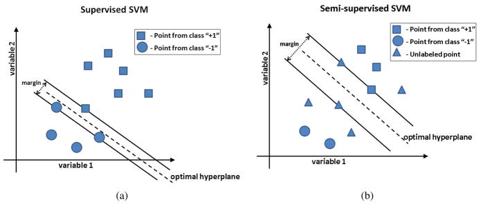
where the slack variables ξ_i are introduced to allow some amount of misclassification in the case of non-separable classes, and constant β implicitly controls the tolerable misclassification error. Figure 2(a) shows a simplified example of the supervised SVM for a two-dimensional problem. Training examples that lie on the margin define the decision boundary and are called support vectors. A more detailed description of the SVM can be found in (Burges, 1998). Notice, that the supervised SVM formulation assumes that labels for all training points are available during training.

Figure 2.

Supervised and semi-supervised SVM. (a) Traditional supervised SVM classification for the simplified case of only two variables. Each symbol represents a brain image. The dashed line represents the hyperplane that correctly classifies the two classes and has the largest margin. All training points must have associated labels; (b) In the semi-supervised SVM, part of the data is unlabeled. The task of semi-supervised SVM is to assign unlabeled points into one of the two classes in such a way, that the resulting classes can be separated by a hyperplane with a large margin.

Semi-supervised SVM, originally introduced as Transductive SVM (TSVM) (Vapnik, 1998), build upon the theory of SVM and consider partially labeled datasets. Given a set of points = {x₁, …, x_l, x_l+1, …, x_n}, where the first l points in are labeled as y_i ∈ {−1, +1} and the labels y_j ∈ {−1, +1} of the remaining u = n − l points are unknown, the task of finding a separating function within the framework of semi-supervised SVM could be formulated as follows:

$$\begin{array}{l}\underset{y_{l+1},\dots ,y_n}{min}\underset{\mathbf{w},b,\xi }{min}\frac{1}{2}{\mathbf{w}}^T\mathbf{w}+{\beta }_l\sum _{i=1}^l{\xi }_i+{\beta }_u\sum _{j=l+1}^n{\xi }_j\\ \mathbf{s}.\mathbf{t}.y_i({\mathbf{w}}^T{\mathbf{x}}_i+b)\ge 1-{\xi }_i,\forall i=1,\dots ,l\\ y_j({\mathbf{w}}^T{\mathbf{x}}_j+b)\ge 1-{\xi }_j,\forall j=l+1,\dots ,n\\ {\xi }_i\ge 0,{\xi }_j\ge 0,\forall i=1,\dots ,l,\forall j=l+1,\dots ,n\end{array}$$ (2)

where constants β_l and β_u reflect prior confidence in labels (y₁, …, y_l) and in the separability of the unlabeled data points, respectively. A simplified example of the semi-supervised SVM is shown in Figure 2(b). In the figure, both labeled and unlabeled data points take part in estimating the optimal separating hyperplane. In the context of semi-supervised SVM, the optimal hyperplane has to both separate the labeled points, as well as to separate unlabeled points into the two classes with a large margin. In our experiments, the two labeled subsets were represented by normal and AD subjects, while MCI subjects were considered to be unlabeled, as they cannot be clearly categorized into “healthy” or “diseased”, and in addition they represent a highly heterogeneous and mixed population. Next, we describe a framework that utilizes semi-supervised SVM to classify patients with MCI.

2.1.2. Semi-supervised pattern classification: Case of MCI

Follow-up evaluations of patients with MCI indicate that a number of them may convert to AD shortly after the baseline evaluation took place. Participants that have not yet converted to AD are usually labeled as non-converters. A classifier can potentially be constructed to classify converters and non-converters using the conversion information as it was done in (Misra et al., 2009). A significant drawback of such approach lies in the fact that a large number of subjects that have not converted to AD at the time of most recent evaluation may convert in the future. Under these circumstances, a semi-supervised approach is more appropriate, as it is designed to handle cases where labels are provided for only part of the data. In our approach, brain MRI images of normal and AD subjects serve as labeled information, and MCI subjects are unlabeled. The task of semi-supervised SVM is then to find a classifying function that both separates AD patients from normal subjects, and provides grouping of MCI patients into normal-like and AD-like.

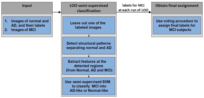
The main steps of our approach are summarized in Figure 3 and are as follows:

Figure 3.

Flowchart of our approach: case of MCI. The input consists of images of normal and AD subjects with their respective labels, and of unlabeled images of MCI subjects. A leave-one-out (LOO) scheme is employed to obtain labels of MCI subjects cross-validated with respect to the labeled data. At each run of the LOO procedure, all but one labeled images are used to detect regions that provide good separation between normal and AD subjects. These regions are used to obtain feature-vector representation of images of normal, AD, and MCI subjects. A linear version of semi-supervised algorithm is then used to obtain labels of the MCI subjects. Finally, a voting scheme is employed to obtain labels for MCI subjects aggregated over all runs of the LOO procedure.

1. Input. The input to the semi-supervised pattern classification approach consists in part of the base-line images of normal and AD subjects with their respective labels. Additionally, base-line images of MCI subjects are considered to be unlabeled and constitute another part of the input. All images were processed as described below in the Materials section of this paper.

2. Leave-one-out semi-supervised classification. We employed a leave-one-out (LOO) scheme for classifying MCI subjects into AD-like and normal-like classes. LOO cross-validation allows to obtain a prediction result that is likely to generalize to an independent data set. The LOO semi-supervised classification procedure of our method has the following components:

   • At every run of leave-one-out procedure we remove one subject from the labeled population (i.e., AD or normal).

   • In order to reduce the dimensionally of the data, we employ the interest region detection approach developed by Fan et al. (Fan et al., 2007). Their method constructs spatial patterns of brain regions that are good discriminators between AD and normal populations. The interest region detection method works by extracting a set of candidate features, and by employing a Support Vector Machine-Recursive Feature Elimination (SVM-RFE) technique to rank computed features according to their effect on the leave-one-out error bound. The procedure in (Fan et al., 2007) accepts images of normal and AD subjects together with their respective labels, and estimates a set of brain regions that are discriminative of AD.

   • With discriminative regions at hand, we extract features at the detected regions from the images of normal, AD and MCI subjects. For a given region, a feature descriptor is extracted by calculating the mean tissue density value in that region. This procedure allows to obtain feature-vector representation of original images, and to reduce the dimensionality of the data to about a hundred dimensions.

   • Finally, during a given run of leave-one-out procedure, the feature-vectors extracted from the images together with the labels of the respective AD and normal subjects serve as the input to the linear semi-supervised SVM algorithm. We implemented the semi-supervised SVM learning procedure described in (Zhao et al., 2008). The learning algorithm in (Zhao et al., 2008) represents the original non-convex problem (2) with a set of nested convex subproblems, and in this way allows for an efficient approximation of the solution to the semi-supervised SVM. MCI subjects that are classified into the same class as the majority of labeled AD patients (i.e., have positive labels) are deemed to be AD-like. Similarly, MCI subjects that are classified into the same class as the majority of normal subjects (i.e., have negative labels) are deemed to be normal-like.

3. Obtain final assignment. At every run of the leave-one-out procedure we obtain labels that may be slightly different for different runs. In order to obtain reliable labels for the MCI subjects we employ the following voting procedure: The final label for a given subject is assigned to be the one that corresponds to the majority of the labels obtained for the subject during all runs of leave-one-out procedure. For a given subject, this final label indicates whether the subject’s brain has AD-like or normal-like structure.

In addition to the labels for the MCI subjects, each run of the leave-one-out procedure allows to obtain the value of the classification function for every MCI patient. This score is equal to the value of the classification function for the specific patient and serves as a biomarker of AD-like brain atrophy patterns. A larger value of the classification function indicates higher similarity to AD for the respective brain’s structure. Averaging values of the classification function over all runs of LOO allows to obtain a stable value of the biomarker of AD for each MCI patient.

Note that, special care may need to be taken in order to reduce the effect of potentially mis-calibrated values of the classification function between cross-validation folds, which can be addressed by converting the classification values to pseudo-probabilities as in (Platt, 1999). We analyzed if assigning final labels based on the sign of the average value of the classification function has different result than the label-voting performed across cross-validation folds. There was no significant difference in the final labels obtained with any of the two approaches, with only 3% of the final labels being different.

Finally, while the above semi-supervised procedure is provided for the problem of classifying MCI subjects, it is in fact general, and can be applied to other studies where there is uncertainty in diagnoses for some individuals.

2.2. Materials

2.2.1. Alzheimer’s Disease Neuroimaging Initiative (ADNI)

Data used in the preparation of this paper was obtained from the ADNI database (www.loni.ucla.edu\ADNI). The goal of ADNI is to recruit 800 adults, ages 55 to 90, to participate in the research – approximately 200 normal control older individuals to be followed for 3 years, 400 people with MCI to be followed for 3 years, and 200 people with early AD to be followed for 2 years. For up-to-date information see www.adni-info.org.

2.2.2. Participants

ADNI participants with structural MR images were part of this analysis. The AD and normal control individuals were exactly the same as in (Fan et al., 2008a), and the MCI individuals as in (Davatzikos et al., 2010), but with the addition of another three MCI subjects. This included 63 control normal (CN) individuals (age range: 75.18 ± 5.39), 54 AD patients (77.407.02), and 242 MCI participants (age range: 74.99 ± 7.38), of which 68 (MCI-C, 76.22 ± 7.20) were classified as having undergone conversion to AD based on changes in Global CDR from 0.5 to 1. The remaining 174 MCI participants (MCI-NC: 74.49 ± 7.41) were classified as non-converters. The MMSE scores (mean ± std. deviation) of MCI-NC and MCI-C at baseline were 27.15 ± 1.93 and 25.75 ± 2.32, respectively. The average time interval between the baseline and the last follow-up scans was 1.95 years. The MMSE scores (mean ± std. deviation) of MCI-NC and MCI-C at baseline were 27.15 ± 1.93 and 25.75 ± 2.32, respectively. 44.12% of MCI-C and 14.71% of MCI-NC had 1 APOE4 (apolipoprotein E) allele, while 37.93% of MCI-C and 9.20% of MCI-NC had 2 APOE4 alleles, respectively. We include the list of ADNI subjects used in our experiments in the supplemental materials.

2.2.3. Images

The dataset included standard T1-weighted images obtained using volumetric 3D MPRAGE or equivalent protocols with varying resolutions (typically 1.25 × 1.25 mm in-plane spatial resolution and 1.2 mm thick sagittal slices). Only images obtained using 1.5 T scanners were used in this study. The sagittal images were preprocessed according to a number of steps detailed under the ADNI website, which corrected for field inhomogeneities and image distortion, and were resliced to axial orientation.

2.2.4. Image analysis

Images were preprocessed according to previously validated and published techniques (Goldszal et al., 1998). The pre-processing steps included: 1) Alignment to the ACPC plane; 2) removal of extra-cranial material (skull-stripping); 3) Tissue segmentation into gray matter (GM), white matter (WM), and cerebrospinal fluid (CSF), using a brain tissue segmentation method proposed in (Pham and Prince, 1999); 5) Formation of regional volumetric maps, named RAVENS maps (Goldszal et al., 1998; Davatzikos et al., 2001; Shen and Davatzikos, 2003), using tissue-preserving image warping (Goldszal et al., 1998). RAVENS maps quantify the regional distribution of GM, WM, and CSF, since one RAVENS map is formed for each tissue type. In particular, if the image warping transformation that registers an individual scan with the template applies an expansion to a GM structure, the GM density of the structure decreases accordingly to insure that the total amount of GM is preserved. Conversely, a RAVENS value increases during contraction, if tissue from a relatively larger region is compressed to fit a smaller region in the template.

Consequently, RAVENS values in the template’s (stereotaxic) space are directly proportional to the volume of the respective structures in the original brain scan. Therefore, regional volumetric measurements and comparisons are performed via measurements and comparisons of the respective RAVENS maps. For example, patterns of GM atrophy in the temporal lobe are quantified by patterns of RAVENS decrease in the temporal lobe in the stereotaxic space. The RAVENS approach has been extensively validated (Goldszal et al., 1998; Davatzikos et al., 2001) and applied to a variety of studies (Resnick et al., 2000, 2003; Beresford et al., 2006a,b; Gur et al., 2005; Stewart et al., 2006). It uses a highly conforming high-dimensional image warping algorithm that captures fine structural details. Moreover, it uses tissue-preserving transformations, which ensures that image warping absolutely preserves the amount of GM, WM and CSF tissue present in an individual’s scan, thereby allowing for local volumetric analysis. In order to minimize longitudinal jitter noise that can be introduced by independently warping each person’s image to the atlas, we first aligned all scans of each individual to his/her baseline scan, via rigid registration based on mutual information. We also minimized the potential biases that can be introduced by reslicing and interpolation, by reslicing each scan exactly one time. The baseline scans were resliced to be parallel to the ACPC plane, and each follow-up was resliced in co-registration with the ACPC aligned baseline scan of the respective participant. Only GM RAVENS maps were used in our experiments.

3. Results

3.1. Effect of unlabeled data

The aim of our first set of experiments is to assess how the presence of unlabeled data affects the classification performance of semi-supervised SVM.

3.1.1. Effect on classification of AD and normal controls

As the diagnostic information for MCI subjects is not reliable in the absence of long-term follow-up evaluations, the classification results obtained for MCI cohort may be difficult to interpret. We therefore started by analyzing the effect of unlabeled data on classification of AD and normal controls if part of AD and control subjects are unlabeled. No MCI subjects were considered at this point of our analysis.

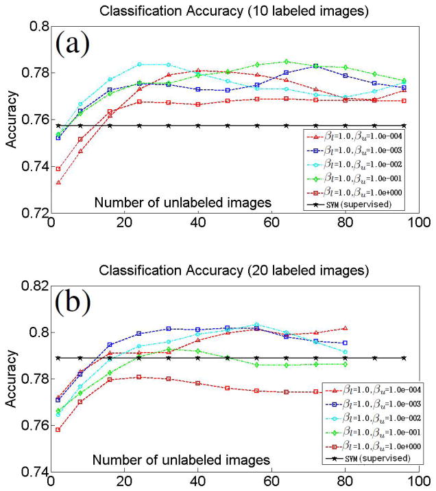
Equal number of AD and control subjects were randomly assigned into the labeled set. Similarly, equal numbers of AD and control subjects were randomly assigned into the unlabeled set. The selected labeled and the unlabeled subsets were disjoint. The plots in Figure 4 display the evolution of leave-one-out classification accuracy for fixed number of labeled images and with increasing number of unlabeled images. The results are averaged for 50 different samplings of labeled and unlabeled subsets. Plots are also shown for different combinations of the semi-supervised SVM parameters β_l and β_u. Additionally, the classification accuracy of the traditional fully-supervised SVM for the specific number of labeled images is also shown. In our experiments, we observed that the performance of the traditional SVM was not significantly affected by the choice of the parameter β in Equation 1, and, therefore, we report the SVM classification accuracy for β = 1.

Figure 4.

Effect of unlabeled data on AD/controls classification. Evolution of leave-one-out classification accuracy for fixed number of labeled images and with increasing number of unlabeled images. Plots obtained for labeled sets of size 10 (a), and 20 (b). Equal number of AD and control subjects were assigned into the labeled set. Similarly, equal numbers of AD and control subjects were always assigned into the unlabeled set. Classification accuracy of traditional SVM using the specific number of labeled images are also provided.

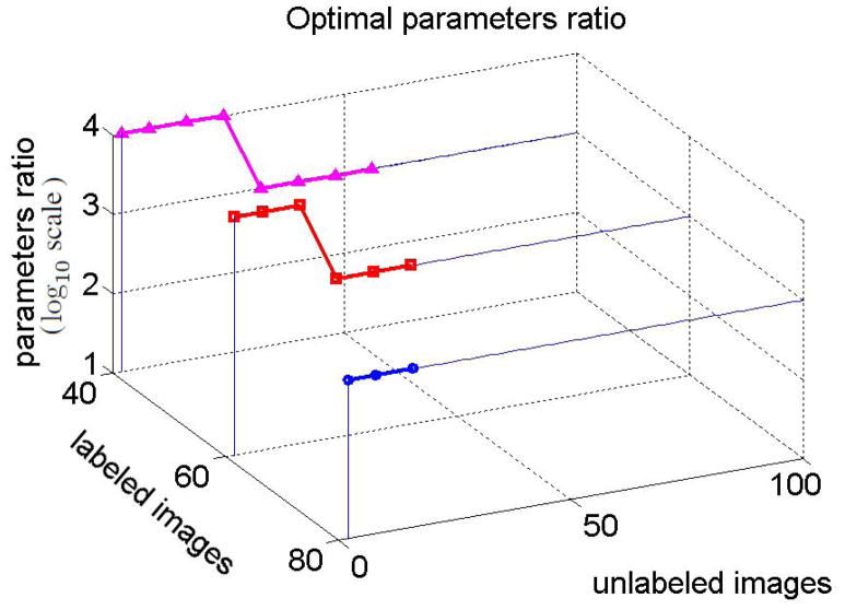
The plots in the Figure suggest that including unlabeled data into the classifier may indeed improve the classification accuracy. However, it is important to select proper semi-supervised SVM parameters. Notice, that if the number of labeled images is not too small, then the choice of parameters where β_l is relatively much higher than β_u results in a better accuracy (i.e., Figure 4(b)). Intuitively, the ratio $\frac{{\beta }_l}{{\beta }_u}$ reflects one’s confidence that the labeled data describes the true data distribution. This confidence is typically higher for larger labeled sets. We estimated the optimal ratio of the semi-supervised SVM parameters that yields highest classification accuracy for a given number of labeled and unlabeled images. Figure 5 shows best parameters ratios estimated for the labeled sets of sizes 40, 60, and 80. The values of the optimal ratio are in the log₁₀ scale, and β_l = 1 in all experiments.

Figure 5.

Optimal ratio $\frac{{\beta }_l}{{\beta }_u}$ that yields highest classification accuracy. The values of the optimal ratio are in the log₁₀ scale.

In the experiment, the larger was the number of selected labeled images, the smaller was the maximum number of available unlabeled images. Nevertheless, it can be inferred from Figure 5 that the optimal ratios are large if the number of labeled images increases. Specifically, when the number of labeled images was 40, 60, or 80, then the optimal ratio of semi-supervised SVM parameters was $\frac{{\beta }_l}{{\beta }_u}={10}^3$ or $\frac{{\beta }_l}{{\beta }_u}={10}^4$.

3.1.2. Effect on classification of MCI

The populations of AD and normal controls are known to be well separable with various approaches consistently achieving high AD/controls classification accuracy (Cuingnet et al., 2010). At the same time, sensitivity and specificity of MRI-based classification of MCI-C and MCI-NC are relatively low. We performed a set of experiments to understand the behavior of semi-supervised SVM in the task of classifying MCI subjects. In this set of experiments all 242 MCI participants formed the unlabeled set. A specific number of AD and control subjects were randomly selected to form the labeled set. We then estimated the accuracy of classifying the unlabeled subjects (i.e., MCI) into “AD-like” and “normal-like”.

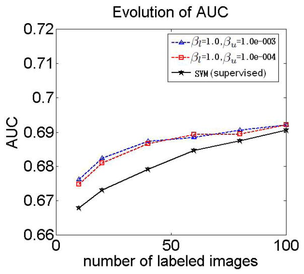
The results in the previous section showed that the choice of semi-supervised parameters where β_l = 1, and β_u = 10⁻³ or β_u = 10⁻⁴, yields the highest accuracy of classifying AD and control subjects if the number of labeled images increases. Figure 6 shows the area under the ROC curve (AUC) for MCI-C/MCI-NC classification obtained for different sizes of the labeled set, and for β_u = 10⁻³ and β_u = 10⁻⁴, and for β_l = 1.

Figure 6.

Effect of unlabeled data on MCI-C/MCI-NC classification. The plot shows AUC for MCI-C/MCI-NC classification obtained for different sizes of the labeled set, and for different parameters β_l = 1, and β_u = 10⁻³ and β_u = 10⁻⁴. Also shown are the results obtained by training a supervised classifier using labeled AD and control images, and then by applying the classifier to the unlabeled data.

Additionally, the plots show the results of MCI-C/MCI-NC classification obtained by training a supervised classifier using labeled AD and control images, and then by applying the classifier to the unlabeled data.

The plot in Figure 6 suggests that the semi-supervised SVM outperforms traditional SVM if the number of labeled images is relatively small. However, due to the uncertainty in labels of MCI-C and MCI-NC participants it is not possible to draw reliable conclusions about the performance of the approach based on the results in Figure 6. In this respect, the results reported in Figure 4 in the previous section better reflect the effects of unlabeled data on the classification performance. Next, we take a closer look at the subpopulations obtained as the result of semi-supervised classification.

3.2. Semi-supervised classification of MCI

In our next set of experiments we considered all available to us 63 control, 54 AD, and 242 MCI participants. As in the previous section, AD and control subjects were considered to be labeled, and MCI subjects were unlabeled. Considering the results in Figure 5, we set β_l = 1.0 and β_u = 0.001, as these parameter provided consistently relatively good classification when the number of labeled images was large. We calculated the number of MCI subjects that converted to AD and, at the same time, were classified as AD-like by our approach. 79.4% of all converters were classified as AD-like. The remaining 21.6% of converters were classified as normal-like. At the same time, 51.7% of non-converters were classified as normal-like, and the remaining 48.3% of non-converters were classified as AD-like. The AUC for the MCI-C/MCI-NC classification was 0.69. Large number of AD-like non-converters may indicate that many of the non-converters will actually convert to AD in the future. The accuracy of the semi-supervised SVM was similar to the accuracy of a fully-supervised classifier trained on AD/controls subjects and applied to MCI, where 78.8% of all converters were classified as AD-like, and 51.0% of non-converters were classified as normal-like. Additionally, the accuracy of the semi-supervised approach in classification of AD/controls was 82.91%, sensitivity was 79.63%, and specificity was 85.71%.

3.2.1. Group comparisons via voxel-based analysis

We performed a series of voxel-wise t-tests to compare the image groups obtained as the result of our proposed semi-supervised classification.

Normal-like MCI vs. AD-like MCI

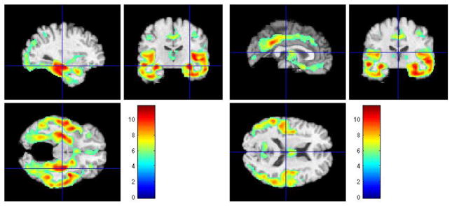
In our first set of voxel-wise t-tests we assessed regional differences in GM between normal-like MCI and AD-like MCI. Figure 7 shows the results of FWE-corrected t-test signifying areas where GM tissue density is greater in normal-like MCI than in ad-like MCI. The values were thresholded at p = 0.05.

Figure 7.

Representative sections with regions of relatively reduced GM in AD-like MCI compared to normal-like MCI, at baseline. FWE-corrected t-test thresholded at p = 0.05. The color-maps indicate the scale for the t-statistic.

Several regions of relatively reduced volumes of GM in normal-like MCI compared to AD-like MCI are evident, including the hippocampus, amygdala, and entorhinal cortex, much of the temporal lobe GM and the insular cortex (especially the superior temporal gyrus), posterior cingulate and precuneous, and orbitofrontal cortex. The inverse contrast in Figure 8 shows increased periventricular gray tissue in AD-like MCI subpopulation, likely due to leukoareosis in AD-like MCI.

Figure 8.

Representative sections with regions of relatively reduced gray-looking tissue in normal-like MCI compared to AD-like MCI, at baseline. FWE corrected t-test thresholded at p = 0.05. The color-maps indicate the scale for the t-statistic.

Normal-like non-converters vs. AD-like non-converters

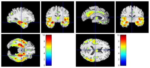
As we mentioned earlier, a large fraction (i.e., 48.3%) of MCI subjects that have not converted to AD during the evaluation period were classified as AD-like. Therefore, it is of interest to assess the regional differences between AD-like and normal-like non-converters, and to verify whether regional differences are consistent with regional differences between AD and normal subjects reported in the existing literature. Figure 9 shows representative sections obtained after applying voxel-wise t-tests, and signifies regions where GM tissue density is higher in normal-like non-converters. The results show that AD-like non-converters exhibit patterns of atrophy that are indicative of AD. This may suggest that AD-like non-converters are more likely to convert to AD in the future.

Figure 9.

Representative sections with regions of relatively reduced GM in AD-like MCI-NC compared to normal-like MCI-NC, at baseline. FWE corrected t-test thresholded at p = 0.05. The color-maps indicate the scale for the t-statistic.

Additionally, the inverse contrast in Figure 10 also shows increased vascular pathology in AD-like non-converters.

Figure 10.

Representative sections with regions of relatively reduced gray-looking tissue GM in normal-like MCI-NC compared to AD-like MCI-NC, at baseline. FWE corrected t-test thresholded at p = 0.05. The color-maps indicate the scale for the t-statistic.

AD-like non-converters vs. AD-like converters

Interestingly, neither FWE-corrected t-test at p < 0.05, nor non-corrected t-test at p < 0.001, showed regions of significant differences between AD-like MCI-NC and AD-like MCI-C. This suggests that subjects with positive values of the classification function have similar patterns of brain tissue loss, regardless of the fact that some of them have not been diagnosed with AD.

3.2.2. Correlation of classification values with age, MMSE, and APOE

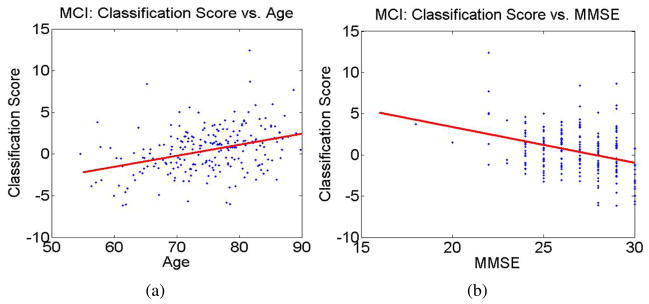
Values of the classification function for MCI subjects increase with age, indicating higher rates of AD-like structure in older individuals (i.e., Figure 11(a)). Correlation coefficient between values of the classification function and age was found to be equal to R = 0.36.

Figure 11.

Correlation of the values of the classification function with age and MMSE. (a) Correlation of classification function values and age (R = 0.36); (b) Correlation of classification function values and MMSE (R = −0.34).

Additionally, individuals with high values of the classification function also have associated low MMSE (i.e., Figure 11(b)). Correlation coefficient between values of the classification function and MMSE was found to be equal R = −0.34.

Additionally, we used measurements from follow-up evaluations and obtained rate of change of MMSE scores for MCI subjects. AD-like MCI showed on average higher rates of decline in MMSE scores. The (mean ± std. deviation) was found to be (−1.36 ± 2.22) in AD-like MCI, and (−0.61 ± 1.77) in normal-like MCI. The significance of difference in rates of MMSE change between AD-like MCI and normal-like MCI was p = 0.023 as indicated by the t-test. As by the cut-off date of our data collection the number of follow-up evaluations in ADNI was limited, and the subjects are followed over a short period of time (i.e., usually 2 follow-up evaluations over a period of 18 months), the change of MMSE change is very noisy. Additional follow-up evaluations will be required to obtain more reliable rates of change of MMSE.

While the correlation of the classification values with age and MMSE scores was intuitive, the distribution of APOE4 alleles in the obtained subgroups of MCI was less conclusive. In particular, 44.17% and 8.33% of AD-like MCI had 1 and 2 APOE4 alleles, respectively, while 35.25% and 13.11% of Normal-like MCI had 1 and 2 APOE4 alleles, respectively.

3.3. Selecting labeled subjects based on extreme clinical scores

Up until now, we assumed that the labels of the labeled data (i.e., AD and CN) were well defined. That is, normal subjects remained normal during the study, and the certainty in the diagnoses of AD was very high. This may not be the case in other studies that lack certainty in the labels. For example, in the studies of normal aging all subjects may be normal, with different subjects exhibiting different levels of cognitive decline (Resnick et al., 2003). To show the potential of the semi-supervised classification in such scenarios we performed an experiment where we considered only MCI subjects from the ADNI, and formed labeled sets using the subjects that corresponded to the extreme values of rates of change in cognitive evaluations. More specifically, out of the 68 MCI-C subjects we selected 20 subjects with the lowest slopes of the MMSE score to represent the positive labeled subset. Similarly, out of the 174 MCI-NC subjects we selected 20 subjects with the highest slopes of the MMSE score to represent the negative labeled subset. The remaining 202 MCI subjects were considered to be unlabeled. Notice, that while we consider only baseline scans, we used cognitive evaluations at the follow-ups to calculate the slopes (i.e., rates of change) of MMSE scores. The mean MSSE slope in the positive labeled subset was −3.73 ± 1.54, and the mean MSSE slope in the negative labeled subset was 1.36 ± 1.03.

Similarly to the previous experiment, we set β_l = 1.0 and β_u = 0.001. It is important to mention that the choice of the parameters β_l and β_u was made based on the analysis of the classifier’s performance on AD/CN classification in Section 3.1.1. As the result, the parameters selection was performed on the set that is not part of the current experiment. After performing the semi-supervised classification within a leave-one-out evaluation scheme we found that the AUC of the MCI-C/MCI-NC classifier was 0.69. At the same time, a fully supervised classifier trained on the selected labeled subsets, and applied to the unlabeled data resulted in AUC equal 0.61. Given that an AUC of 0.5 represents classification by chance, the improvement provided by semi-supervised approach over the fully-supervised method is quite significant.

4. Discussion and Conclusion

In this paper, we explored the potential of semi-supervised approaches to classify individuals with progressive disorders in the absence of long-term follow-up evaluations. We applied a strategy based on semi-supervised SVM in the ADNI study, and obtained an indicator of AD-like atrophy patterns that has good predictive power of conversion from MCI to AD. The principal difference between our semi-supervised approach and related fully-supervised techniques lies in the fact that the supervised approaches assume that the heterogeneous structure of the population is known. In the case of MCI, these supervised approaches assume that the population of MCI consists of MCI-converters and MCI-non-converters. In contrast, our semi-supervised approach does not make strong assumptions about the structure of MCI, but rather attempts to disentangle the heterogeneity of MCI via high-dimensional pattern analysis.

Analysis of volumetric differences of AD-like and normal-like MCI showed that AD-like MCI had reduced GM volumes in a number of brain regions, including superior, middle and inferior temporal gyri, anterior hippocampus and amygdala, orbitofrontal cortex, posterior cingulate and the adjacent precuneous, insula and fusiform gyrus (i.e., Figure 7). Moreover, pronounced was the larger size of the temporal horns of the ventricles (i.e., Figure 8). These results indicate that AD-like MCI may have already reached levels of widespread and significant brain atrophy at baseline.

Similar, albeit somewhat less severe, deferences were observed between normal-like MCI-NC and AD-like MCI-NC (i.e., Figures 9 and 10). These results indicate that the pathological changes in the AD-like MCI-NC are significantly more progressed, and that this particular group of non-converters is likely to convert to AD in the future.

Additionally, we observed that there is no significant difference in the patterns of atrophy in AD-like MCI-NC and AD-like MCI-C. This suggests that the AD-like MCI share the same patterns of atrophy regardless of the most recent conversion status. A more prolonged evaluation of MCI-NC subjects from ADNI is required to validate the hypothesis that AD-like MCI-NC are more likely to convert to AD.

The classification function derived from the semi-supervised SVM was found to have relatively good sensitivity, in that almost all MCI-C patients where classified as AD-like. Not unexpectedly, specificity was limited. This is largely due to the short follow-up periods in this study. Since MCI patients convert to AD at a rate of approximately 15% annually, it is anticipated that many MCI-NC will convert to AD in the near future. Although future studies with longer follow-up times will refine our estimates of specificity, our results indicated that positive values of the classification function in MCI-NC were associated with lower MMSE scores, and with higher rates of decline in MMSE scores.

The results in Figure 6 indicate that if the labeled subsets are formed from the AD and CN subjects, then the semi-supervised classifier only slightly outperforms its supervised counterpart. At the same time, if AD and CN subjects are not available, and the labeled subsets are formed from the MCI subjects based on the extreme rates of changes in cognitive scores, then the difference in classification performance is quite significant. We found that AUC of the semi-supervised classifier was equal to 0.69, while the supervised classifier yielded AUC equal to 0.61. Overall, the MCI-C/MCI-NC classification problem is characterized by exceptionally low separability and difficulty, and predicting short-term cognitive decline from baseline scans is bound to be very limited, albeit it is largely improved by semi-supervised classification. The large difference in performance of the classifiers can be explained by the fact that the labeled data in the experiment in Section 3.3 was selected based on the extreme values of the MMSE slopes. MMSE scores are very noisy and are not sufficiently good indicators of conversion to AD. As the result, the labels of the subjects in the labeled subsets were uncertain, which may have hampered the performance of the fully-supervised classifier. At the same time, the availability of the unlabeled data allows the semi-supervised classifier to better learn the manifold of MCI subjects, and hence to build a more reliable separation function. On the other hand, if the labeled sets are formed from AD and CN subjects, the labels of the subjects in the labeled subsets are much more reliable, and given a sufficiently large number of labeled subjects it is possible to obtain a fully-supervised classifier that performs on a par with the semi-supervised approach.

As it can be seen from our experiments, the choice of the semi-supervised SVM parameters has significant effect on the classification performance. A possible strategy to selecting the parameters would be to use participants with longer follow-up evaluations, and hence more certain labels, in the parameters optimization stage. Unfortunately, due to the short follow-up period in the ADNI, the certainty in the labels of MCI subjects is questionable. At the same time, some studies such as the Baltimore Longitudinal Study of Aging (BLSA) (Resnick et al., 2003) have the follow-up period of more than fifteen years, and therefore may allow to select a validation set with reliable ground truth data on which the optimal parameters can be found.

Finally, we would like to comment on the AD/controls classification performance of both traditional and semi-supervised SVM. Existing literature suggests that differences in processing protocols, classification algorithms and feature selection procedures may results in significantly different classification accuracy ranging from less than 80% in some cases (Cuingnet et al., 2010), to up to 90% in others (Misra et al., 2009). In this respect, our AD/controls classification results are moderate. This can be attributed in part to the fact that due to the complexity of the semi-supervised SVM learning problem in 2, we had to restrict our comparative analysis to linear versions of both semi-supervised and traditional SVM.

In summary, we investigated the ability of semi-supervised classification to address specific challenges that arise in studies of progressive disorders and that are due to uncertainty in diagnostic information. The main goal of our paper was to explore whether semi-supervised analysis of MRI data is more preferable to commonly used fully-supervised paradigm under similar conditions. Our analysis suggests that in some scenarios semi-supervised strategy may be more preferable. Specifically, if the number of labeled images is small, semi-supervised approach appears to yield higher classification accuracy. Application of our proposed approach to the problem of classifying MCI subjects within a short-follow-up study yielded encouraging results. The results indicate that pathological patterns can be accurately detected and quantified even if training information is limited. The fact that our results agree with findings obtained using fully supervised approaches may serve as additional computational justification for the assumptions made by these approaches. While in this paper we applied the semi-supervised classification approach to the problem of identifying patterns of AD-like pathology in subjects with MCI, our proposed framework can also be applied to analyzing other progressive disorders. In the future we plan to further explore the potential of semi-supervised classification in the studies of aging, as well as in studies of other diseases.

References

- Bain LJ, Jedrziewski K, Morrison-Bogorad M, Albert M, Cotman C, Hendrie H, Trojanowski JQ. Healthy brain aging: A meeting report from the sylvan m. cohen annual retreat of the university of pennsylvania institute on aging. Alzheimer’s and Dementia. 2008;4 (6):443–446. doi: 10.1016/j.jalz.2008.08.006. [DOI] [PMC free article] [PubMed] [Google Scholar]
- Beresford TP, Arciniegas DB, Alfers J, Clapp L, Martin B, Beresford HF, Du Y, Liu D, Shen D, Davatzikos C, Laudenslager ML. Hypercortisolism in alcohol dependence and its relation to hippocampal volume loss. J Stud Alcohol. 2006a;67 (6):861–7. doi: 10.15288/jsa.2006.67.861. [DOI] [PubMed] [Google Scholar]
- Beresford TP, Arciniegas DB, Alfers J, Clapp L, Martin B, Du Y, Liu D, Shen D, Davatzikos C. Hippocampus volume loss due to chronic heavy drinking. Alcohol Clin Exp Res. 2006b;30 (11):1866–70. doi: 10.1111/j.1530-0277.2006.00223.x. [DOI] [PubMed] [Google Scholar]
- Burges CJC. A tutorial on support vector machines for pattern recognition. Data Mining and Knowledge Discovery. 1998;2:121–167. [Google Scholar]
- Cuingnet R, Gerardin E, Tessieras J, Auzias G, Lehericy S, Habert M-O, Chupin M, Benali H, Colliot O. Automatic classification of patients with alzheimer’s disease from structural mri: A comparison of ten methods using the adni database. Neuroimage. 2010 doi: 10.1016/j.neuroimage.2010.06.013. [DOI] [PubMed] [Google Scholar]
- Davatzikos C, Bhatt P, Shaw LM, Batmanghelich KN, Trojanowski JQ. Prediction of mci to ad conversion, via mri, csf biomarkers, and pattern classification. Neurobiology of Aging. 2010 doi: 10.1016/j.neurobiolaging.2010.05.023. In Press, Corrected Proof. [DOI] [PMC free article] [PubMed] [Google Scholar]
- Davatzikos C, Genc A, Xu D, Resnick SM. Voxel-based morphometry using the ravens maps: Methods and validation using simulated longitudinal atrophy. NeuroImage. 2001;14 (6):1361–1369. doi: 10.1006/nimg.2001.0937. [DOI] [PubMed] [Google Scholar]
- Davatzikos C, Xu F, An Y, Fan Y, Resnick SM. Longitudinal progression of Alzheimer’s-like patterns of atrophy in normal older adults: the SPARE-AD index. Brain. 2009;132 (8):2026–2035. doi: 10.1093/brain/awp091. [DOI] [PMC free article] [PubMed] [Google Scholar]
- Duchesne S, Bocti C, Sousa KD, Frisoni GB, Chertkow H, Collins DL. Amnestic mci future clinical status prediction using baseline mri features. Neurobiology of Aging. 2008a doi: 10.1016/j.neurobiolaging.2008.09.003. In Press, Corrected Proof. [DOI] [PubMed] [Google Scholar]
- Duchesne S, Caroli A, Geroldi C, Barillot C, Frisoni G, Collins D. Mri-based automated computer classification of probable ad versus normal controls. IEEE Trans Med Imaging. 2008b April;27 (4):509–520. doi: 10.1109/TMI.2007.908685. [DOI] [PubMed] [Google Scholar]
- Ecker C, Rocha-Rego V, Johnston P, Mourao-Miranda J, Marquand A, Daly EM, Brammer MJ, Murphy C, Murphy DG. Investigating the predictive value of whole-brain structural mr scans in autism: A pattern classification approach. NeuroImage. 2010;49 (1):44–56. doi: 10.1016/j.neuroimage.2009.08.024. [DOI] [PubMed] [Google Scholar]
- Fan Y, Batmanghelich N, Clark CM, Davatzikos C. Spatial patterns of brain atrophy in mci patients, identified via high-dimensional pattern classification, predict subsequent cognitive decline. NeuroImage. 2008a;39 (4):1731–1743. doi: 10.1016/j.neuroimage.2007.10.031. [DOI] [PMC free article] [PubMed] [Google Scholar]
- Fan Y, Gur RE, Gur RC, Wu X, Shen D, Calkins ME, Davatzikos C. Unaffected family members and schizophrenia patients share brain structure patterns: a high-dimensional pattern classification study. Biol Psychiatry. 2008b;63 (1):118–24. doi: 10.1016/j.biopsych.2007.03.015. [DOI] [PMC free article] [PubMed] [Google Scholar]
- Fan Y, Resnick SM, Wu X, Davatzikos C. Structural and functional biomarkers of prodromal alzheimer’s disease: A high-dimensional pattern classification study. NeuroImage. 2008c;41 (2):277–285. doi: 10.1016/j.neuroimage.2008.02.043. [DOI] [PMC free article] [PubMed] [Google Scholar]
- Fan Y, Shen D, Gur RC, Gur RE, Davatzikos C. Compare: Classification of morphological patterns using adaptive regional elements. IEEE Trans Med Imaging. 2007;26 (1):93–105. doi: 10.1109/TMI.2006.886812. [DOI] [PubMed] [Google Scholar]
- Goldszal AF, Davatzikos C, Pham DL, Yan MXH, Bryan RN, Resnick SM. An image-processing system for qualitative and quantitative volumetric analysis of brain images. Journal of Computer Assisted Tomography. 1998 April;22 (5):827–837. doi: 10.1097/00004728-199809000-00030. [DOI] [PubMed] [Google Scholar]
- Gur R, Davatzikos C, Shen D, Wu X, Fan Y, PH, Turetsky B, Gur R. Whole-brain deformation based morphometry mri study of schizophrenia. Schizophrenia Bulletin. 2005;31(2):408–408. [Google Scholar]
- Hebert LE, Beckett LA, Scherr PA, Evans DA. Annual incidence of alzheimer disease in the united states projected to the years 2000 through 2050. Alzheimer Dis Assoc Disord. 2001;15 (4):169–173. doi: 10.1097/00002093-200110000-00002. [DOI] [PubMed] [Google Scholar]
- Hinrichs C, Singh V, Mukherjee L, Xu G, Chung MK, Johnson SC. Spatially augmented lpboosting for ad classification with evaluations on the adni dataset. NeuroImage. 2009;48 (1):138–149. doi: 10.1016/j.neuroimage.2009.05.056. [DOI] [PMC free article] [PubMed] [Google Scholar]
- Joachims T. Transductive inference for text classification using support vector machines. Proceedings 16th International Conference on Machine Learning; 1999. pp. 200–209. [Google Scholar]
- Kloppel S, Stonnington CM, Chu C, Draganski B, Scahill RI, Rohrer JD, Fox NC, Jack CR, Ashburner J, Frackowiak RSJ. Automatic classification of mr scans in alzheimer’s disease. Brain. 2008 March;131 (3):681–689. doi: 10.1093/brain/awm319. [DOI] [PMC free article] [PubMed] [Google Scholar]
- McEvoy LK, Fennema-Notestine C, Roddey JC, Hagler DJ, Holland D, Karow DS, Pung CJ, Brewer JB, Dale AM. Alzheimer Disease: Quantitative Structural Neuroimaging for Detection and Prediction of Clinical and Structural Changes in Mild Cognitive Impairment1. Radiology. 2009;251 (1):195–205. doi: 10.1148/radiol.2511080924. [DOI] [PMC free article] [PubMed] [Google Scholar]
- Misra C, Fan Y, Davatzikos C. Baseline and longitudinal patterns of brain atrophy in mci patients, and their use in prediction of short-term conversion to ad: Results from adni. NeuroImage. 2009 February;44 (4):1415–1422. doi: 10.1016/j.neuroimage.2008.10.031. [DOI] [PMC free article] [PubMed] [Google Scholar]
- Pham DL, Prince JL. Adaptive fuzzy segmentation of magnetic resonance images. IEEE Trans Med Imaging. 1999;18 (9):737–752. doi: 10.1109/42.802752. [DOI] [PubMed] [Google Scholar]
- Platt JC. Probabilistic outputs for support vector machines and comparisons to regularized likelihood methods. Advances in Large Margin Classifiers. 1999:61–74. [Google Scholar]
- Resnick SM, Goldszal AF, Davatzikos C, Golski S, Kraut MA, Metter EJ, Bryan RN, Zonderman AB. One-year Age Changes in MRI Brain Volumes in Older Adults. Cereb Cortex. 2000;10 (5):464–472. doi: 10.1093/cercor/10.5.464. [DOI] [PubMed] [Google Scholar]
- Resnick SM, Pham DL, Kraut MA, Zonderman AB, Davatzikos C. Longitudinal magnetic resonance imaging studies of older adults: A shrinking brain. J Neurosci. 2003 April;23 (8):3295–3301. doi: 10.1523/JNEUROSCI.23-08-03295.2003. [DOI] [PMC free article] [PubMed] [Google Scholar]
- Shen D, Davatzikos C. Very high-resolution morphometry using mass-preserving deformations and hammer elastic registration. NeuroImage. 2003;18 (1):28–41. doi: 10.1006/nimg.2002.1301. [DOI] [PubMed] [Google Scholar]
- Stewart WF, Schwartz BS, Davatzikos C, Shen D, Liu D, Wu X, Todd AC, Shi W, Bassett S, Youssem D. Past adult lead exposure is linked to neurodegeneration measured by brain MRI. Neurology. 2006;66 (10):1476–1484. doi: 10.1212/01.wnl.0000216138.69777.15. [DOI] [PubMed] [Google Scholar]
- Vapnik VN. The nature of statistical learning theory. Springer-Verlag New York, Inc; New York, NY, USA: 1995. [Google Scholar]
- Vapnik VN. Statistical Learning Theory. Wiley-Interscience; Sep, 1998. [Google Scholar]
- Vemuri P, Wiste HJ, Weigand SD, Shaw LM, Trojanowski JQ, Weiner MW, Knopman DS, Petersen RC, Jack CRJ behalf of the Alzheimer’s Disease Neuroimaging Initiative, O. MRI and CSF biomarkers in normal, MCI, and AD subjects: Diagnostic discrimination and cognitive correlations. Neurology. 2009;73 (4):287–293. doi: 10.1212/WNL.0b013e3181af79e5. [DOI] [PMC free article] [PubMed] [Google Scholar]
- Zhao B, Wang F, Zhang C. Cuts3vm: a fast semi-supervised svm algorithm. KDD ’08: Proceeding of the 14th ACM SIGKDD international conference on Knowledge discovery and data mining; New York, NY, USA: ACM; 2008. pp. 830–838. [Google Scholar]
Associated Data
This section collects any data citations, data availability statements, or supplementary materials included in this article.