Binocular Vision

Abstract

This essay reviews major developments –empirical and theoretical –in the field of binocular vision during the last 25 years. We limit our survey primarily to work on human stereopsis, binocular rivalry and binocular contrast summation, with discussion where relevant of single-unit neurophysiology and human brain imaging. We identify several key controversies that have stimulated important work on these problems. In the case of stereopsis those controversies include position versus phase encoding of disparity, dependence of disparity limits on spatial scale, role of occlusion in binocular depth and surface perception, and motion in 3D. In the case of binocular rivalry, controversies include eye versus stimulus rivalry, role of “top-down” influences on rivalry dynamics, and the interaction of binocular rivalry and stereopsis. Concerning binocular contrast summation, the essay focuses on two representative models that highlight the evolving complexity in this field of study.

Introduction

The 25^th Anniverary Issue of Vision Research included two essays covering binocular vision, both devoted almost entirely to stereopsis. Bishop and Pettigrew (1986) provided a lively chronology of the events leading up to and following the discovery of disparity-selective neurons in cat and monkey (a saga in which both authors were central players). Bela Julesz (1986) treated readers to a first-hand account of the development and refinement of the random-dot stereogram (RDS) and the implications from discoveries using those ground-breaking probes of stereopsis. Julesz s essay also briefly commented on the relation between stereopsis and binocular rivalry.

How has the landscape portrayed in those two essays changed in the 25 years since they were written? Answering that question is our challenge in this 50^th Anniversary essay on binocular vision. And challenging it will be: the field of binocular vision has been remarkably active the last twenty-five years, but page limitations preclude a high-resolution picture of the changes in that landscape. Rather, we must offer a low-resolution overview that highlights some (but certainly not all) of the remarkable discoveries and important theoretical advances. For those seeking a more detailed description of discoveries and advances, there are some excellent books, chapters and reviews that fill in the details missing in this essay, and we will list those sources within the relevant sections. Alas, there are some topics that we will not touch upon at all, even though they fall within the domain of binocular vision. Those include perceived visual direction (Erkelens & van de Grind, 1994), vergence eye movements (Maxwell & Schor, 2006) and clinical disorders in binocular vision (Steinman et al., 2000). Fortunately, there is a comprehensive survey of binocular vision published by Howard and Rogers (2002), and that encyclopedic book offers in-depth overviews of all topics falling under the rubric binocular vision; serious students of binocular vision should consider owning this important book.¹

Stereopsis

As evidenced by the two essays on stereopsis published in the 25th anniversary issue, research on the topic back then focused heavily on RDSs (and the corollary issue of local vs global stereopsis) and on registration of horizontal disparities by single neurons in V1. In their essay, Bishop and Pettigrew (1986) did acknowledge vertical disparities could contribute to estimates of absolute distance, something horizontal disparity alone cannot do (Longuet-Higgins, 1982). This acknowledgment was occasioned, in part, by the growing realization that receptive fields of V1 binocular neurons frequently had vertical, not just horizontal, disparity tuning. The importance of vertical disparity in human stereopsis was indeed substantiated in subsequent work (e.g., Porrill et al., 1999). Bishop and Pettigrew also anticipated two of the major advances highlighted later in this section, the extension of disparity analysis to higher visual areas and the analysis of receptive field substructure promoting disparity selectivity. So, how has our understanding of stereopsis advanced since publication of those two essays? To set the stage for highlighting what we construe to be some of the major developments in the field, let s start by considering a major shift in thinking about the nature of disparity coding.

Twenty-five years ago, a popular idea, sparked by psychophysical (Richards, 1971) and electrophysiological (Poggio, 1984) evidence, was that disparity processing is achieved by just four channels: tuned excitatory (zero disparity), near, far, and tuned inhibitory (inhibition of zero by near and far). This idea metaphorically called to mind color vision, in that a small number of tuned channels spanned the entire range of relevant stimulus values (wavelengths in the case of color, disparities in the case of stereopsis). But as applied to stereopsis, that idea was subsequently abandoned based on psychophysical and computational modeling. For example, disparity specific adaptation (Stevenson et al., 1992) and subthreshold summation (Cormack et al., 1993) indicated the existence of a relatively large number of disparity channels with preferred disparities covering a wide range. According to psychophysically derived estimates, channel bandwidths were narrow at the horopter and grew larger with disparity, both crossed and uncrossed. In addition, data pointed to the existence of inhibitory zones adjacent to the peak disparity tuning. Evidence for multi-channel disparity tuning also received support from computational modeling (e.g., Lehky & Sejnowski, 1990). By the end of the 20^th century, the four-channel model had been supplanted by models in which disparity mechanisms formed a continuum more like that found for orientation, motion direction and spatial frequency. This new view, incidentally, was endorsed by one of the original proponents of the four-channel model, Gian Poggio (1995). At about the same time, those studying stereopsis began paying more attention to the distinction between absolute and relative disparity, in particular the likelihood that the two were represented in distinct neural populations (e.g., Cumming & Parker, 1999). One compelling observation underscoring the distinction between the two is that large changes in absolute disparity go unnoticed when relative disparity remains constant (Erkelens & Collewijn, 1985).

What, then, were key areas of discovery in stereopsis over the past 25 years?

Cortical Pathways involved in Stereopsis

The original descriptions of disparity selectivity were based on single-unit recordings from primary visual cortex of the cat (reviewed by Bishop & Pettigrew, 1986). With the emergence of evidence for dorsal and ventral cortical pathways, it was natural to wonder how stereopsis was represented beyond V1. Based on macaque V2 physiology and human psychophysics, Livingstone and Hubel (1987) proposed that stereopsis and motion were represented only within the magnocellular stream and, by implication, were thus represented in dorsal stream areas including MT. While both disparity and motion are indeed represented in macaque MT (DeAngelis & Uka, 2003) and interact there (Bradley et al., 1995), we now know that stereo information is represented within both the dorsal and ventral pathways of macaques (see Parker, 2007, for a summary of relevant data). As well, stereo-processing can be performed even when the magnocellular system is lesioned using injections of ibotenic acid targeting specific layers of the LGN (Schiller et al., 1991); this finding, too, undermines the proposal linking stereopsis exclusively to the magnocellular pathway and, moreover, indicates that mechanisms involved in color vision play a role in stereopsis, as implied by psychophysical results (e.g., Jordan et al. 1990).

With the advent of brain imaging –in particular, positron emission tomography (PET) and functional magnetic resonance imaging (fMRI) -- it became possible to study the cortical distribution of stereoscopic processing in the human brain (e.g., Gulyás & Roland, 1994) and in the macaque brain (Sereno et al., 2002). Those studies confirmed that disparity-related activations are distributed throughout both the dorsal and ventral visual streams, demonstrating the ubiquity of stereo processing within the brain and, by implication, its importance in vision. Moreover, some of those brain imaging studies were able to shed additional light on the nature of distributed disparity processing. To give two examples, Neri et al. (2004) used an fMRI adaptation paradigm together with stimuli comprising two transparent depth planes so that absolute and relative disparities could be manipulated independently. Their results showed greater adaptation to absolute disparity in the dorsal pathway, including MT+, but equal adaptation in the ventral pathway including V4. More recently Preston et al. (2008) used fMRI to discover that areas within the dorsal pathway encode metric disparity, whereas areas in the ventral pathway primarily encode disparity sign, i.e. near/far categorical disparity. While more remains to be learned, it is clear that disparity information is represented differentially in the two major visual processing streams.

Additional fMRI studies of dorsal and ventral stream disparity processing and of binocular rivalry are discussed in the following sections of this review.

Position versus phase disparity

Influenced by the work of Ogle (Ogle, 1950) and Julesz (1971), along with basic geometric considerations, only position disparity was considered relevant 25 years ago. This constitutes the case where left (L) and right (R) monocular receptive fields feeding into a binocular cortical unit are identical in shape and vary only in horizontal retinal position. Using vertical Gabor functions as a convenient example, the horizontal receptive field profiles of L and R inputs would be:

$${\text{RF}}_{\text{L}}=exp\left(-{\text{x}}^2/{\sigma }^2\right)cos(\omega \text{x})$$ (1)

$${\text{RF}}_{\text{R}}=exp\left(-{(\text{x}-\text{d})}^2/{\sigma }^2\right)cos(\omega (\text{x}-\text{d)})$$ (2)

where x is horizontal location, σ is the space constant of the Gaussian envelope, and d is the disparity. These left and right monocular receptive fields are depicted in Figure 1A. Note that disparity d can be arbitrarily large, although this can lead to false matches.

Figure 1.

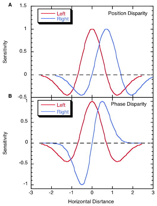
Horizontal receptive field profiles of vertically oriented left eye (red) and right eye (blue), receptive fields. A. A binocular unit combining responses of these two monocular units, which are identical except for a position shift, would be sensitive to a position disparity of approximately 0.8 horizontal distance units. B. Horizontal receptive field profiles of vertically oriented monocular receptive fields with even and odd symmetry. A binocular unit receiving excitation from these two would be sensitive to a 90° inter-ocular phase shift. Note that the two monocular profiles, in virtue of being phase shifted, have different optimal stimuli.

The advent of size or spatial frequency tuning of visual units raised the possibility of phase tuning as an alternative, and this was effectively exploited by several laboratories. In the monocular phase difference scenario, left and right monocular receptive fields can be described as Gabor functions with a phase shift:

$${\text{RF}}_{\text{L}}=exp\left(-{\text{x}}^2/{\sigma }^2\right)cos(\omega \text{x})$$ (3)

$${\text{RF}}_{\text{R}}=exp\left(-{\text{x}}^2/{\sigma }^2\right)cos(\omega \text{x}+\phi )$$ (4)

where ϕ is the phase shift. Due to the periodicity of cosines, ϕ ≤ π, as this is the phase at which the positive peaks of the monocular receptive fields are maximally separated. Phase disparity is depicted in Figure 1B, where an even symmetric receptive field for one eye (left, in the example shown) is paired with an odd symmetric receptive field (ϕ = π/2) driven by the other eye (right eye in the example). The spatial disparity producing the peak response is ϕ/ω. Odd and even symmetry in the monocular receptive fields is not necessary, nor is a π/2 inter-ocular phase shift. Note, however, that as the phase shift approaches ϕ = ±π (where RF_L = −RF_R), two equal but opposite matches between positive response regions of the receptive fields become equally prominent.

The construction of disparity sensitive cells is generally conceptualized as summation of responses from left (L) and right (R) receptive fields followed by squaring (Ohzawa et al., 1990):

$$\mathit{Binoc}={(L(x)+R(x))}^2=L^2(x)+R^2(x)+2L(x)R(x)$$ (5)

Note that this computation implemented by neurons would require the sum of responses from two pairs of binocular simple cells, one with on-centers and the other with off centers, each with a threshold and with squaring only applied to above threshold responses. Assuming spatial pooling over a small range of the horizontal position x, the result of the computation in Equation 5 may be regarded as representing responses of a contrast polarity independent complex cell. Finally, note that the first two terms in Equation (5) represent the summed monocular inputs, while the final term represents the cross-correlation between L and R filtered responses. Clearly, the strongest binocular response will occur when the monocular stimuli are optimal for the position offset or phase difference of the respective receptive fields.

Neurophysiological evidence for phase encoding was first obtained in cat visual cortex (Ohzawa et al., 1990; DeAngelis et al., 1991) and was subsequently verified in macaques (Livingstone & Tsao, 1999; Smith et al., 1997). There is also psychophysical evidence for phase encoding, at least at higher spatial frequencies (Edwards & Schor, 1999) and for wide field gratings (Morgan & Castet, 1997). Further, there are now established computational models of disparity selectivity for complex cortical cells. These involve squaring and summing the monocular inputs as indicated above followed by pooling over spatial regions. This constitutes a disparity energy model generalization of pioneering motion energy models (Adelson & Bergen, 1985), and in the context of stereopsis versions of this model account for hallmark characteristics including disparity-gradient limits and stereo-resolution (Nienborg et al., 2004; Filippini & Banks, 2009).

Position and phase disparity have different characteristics. Although position disparity can in principle be arbitrarily large, phase disparity reaches a maximum at a spatial phase shift of π, which is one half cycle of the peak spatial frequency and the point at which matching ambiguity sets in. With phase disparity there can be only correct matches (or no matches) within a π/2 or quarter-cycle range. However, it has been known for just over 25 years that fusion without diplopia is possible for much larger disparities at high spatial frequencies (Schor et al., 1984). This indicates one of two things: either the visual system uses large position disparities in addition to phase disparities to expand the fusion range, or else disparity information on lower spatial frequency scales constrains processing on higher frequency scales, a coarse-to-fine disparity computation. Before considering interactions across spatial frequency scales, we first examine a controversy regarding the role of phase disparity.

Qian and colleagues have argued that phase disparity detectors provide significantly more accurate population responses for disparities within the phase range 0 to π (Qian & Zhu, 1997). This conclusion is based on calculations using Gabor receptive fields as described above, and their calculations show that the response of a population of phase disparity units is much more sharply peaked than the comparable response of position disparity units. Accordingly, they argued that the visual system ought to utilize phase disparity because of its superior accuracy at modest disparities. It is unclear, however, whether this conclusion is valid for all non-Gabor receptive field profiles, so further work on this topic would be useful.

In contrast to Qian and colleagues, Read and Cumming (2007) have advocated a very different view, motivated by a consideration evident from the monocular receptive field profiles in Figure 1B. Due to the different receptive field shapes, the optimal stimuli for phase disparity in the two eyes will be inherently different. Accordingly, Read and Cumming argued that phase disparity between shifted but identical image features cannot in fact occur in natural images. Instead, they argued that false matches, produced by similar but non-identical monocular image features, would be optimally detected by phase disparity units. Indeed, they showed that phase disparity units are more strongly activated by false matches in natural images than are position disparity units. This led them to propose a neural model in which phase disparity units identify false stereo matches due to their different receptive field profiles, while the maximum response of position disparity units encodes the true disparity. Their model shows that the elimination of maximum phase disparity responses (presumably via inhibition) can unveil the true position disparity, even over many cycles of the optimum spatial frequency (Read & Cumming, 2007).

Two points emerge from these alternative interpretations. First, the physiological evidence clearly shows that both phase and position disparity neurons are present in V1 (Ohzawa et al., 1990; DeAngelis et al., 1991), so stereo computations surely must somehow employ both. Second, there is a major disagreement over whether phase disparity provides the greatest accuracy (Qian & Zhu, 1997) with position disparity playing another role (see next section), or whether position disparity is most accurate with phase disparity aiding in the elimination of false targets (Read & Cumming, 2007). Much of the work fueling this debate is computational, so future psychophysical and physiological experiments are critical for resolving the debate.

Disparity Interactions Across Spatial Scales

To reiterate, position disparities can be arbitrarily large, while phase disparities are limited to a maximum of ±π. In addition, low spatial frequencies support a larger position disparity range than high spatial frequencies (Schor et al., 1984). However, high spatial frequencies can be fused over a much greater range than that permitted by phase disparity on a single spatial frequency scale. This means either that low spatial frequency scales must somehow aid in processing of large disparities on higher scales, or else large position disparities must somehow aid in processing of high spatial frequency phase disparities. We first discuss psychophysical evidence for coarse-to-fine disparity interactions and then consider computational models for these interactions.

The psychophysical evidence that coarse-to-fine interactions are important to fusion of large disparities at high spatial frequencies comes from several sources. One study combined a low spatial frequency D6 (sixth derivatives of Gaussians) with a high spatial frequency D6 and examined the effect of low frequency defined disparity on high spatial frequency increment thresholds (Rohaly & Wilson, 1993). Results showed that low spatial frequency information does indeed constrain the fusion range at high spatial frequencies. However, the data did not support the hypothesis that low spatial frequencies shift the processing of high spatial frequencies into their optimal range. A second study examined disparity averaging using combinations of high and low spatial frequency gratings at the same or different orientations (Rohaly & Wilson, 1994). The data showed that disparities were averaged if the low and high frequency components were separated by less than 3.5 octaves in spatial frequency and 30° in orientation. Beyond this spatial frequency and orientation range, there was no averaging, and depth transparency was seen. In addition, the weighting of the low and high spatial frequency disparity information was a smoothly varying function of their relative contrasts.

A further study examined coarse-to-fine disparity interactions by measuring the fusion range (defined by diplopia thresholds) for high spatial frequency D6 stimuli superimposed on low spatial frequency gratings (Wilson et al., 1991). A high spatial frequency D6 could only be fused within a disparity range centered on the disparity defined by the low spatial frequency grating, even when that grating was tilted in depth. High spatial frequency gratings did not similarly constrain the disparity range for low spatial frequency D6s, thus suggesting a unidirectional stereo processing strategy from coarse to fine. However, evidence for fine to coarse interactions has also been reported (Smallman, 1995). A possible resolution is provided by a physiological study that reported both coarse to fine disparity interactions as well as fine to coarse, with the former being stronger than the latter (Menz & Freeman, 2003).

Spatial frequency interactions clearly occur between scales within about 2.0 octaves of one another, and coarse-to-fine disparity interactions represent a major part of these interactions. Accordingly, a number of computational models introduced coarse-to-fine interactions as a means of extending the processing range at high spatial frequencies. One of those models proposed that both disparity position and phase ambiguities were resolved by pooling disparity responses across spatial frequency and orientation (Fleet et al., 1996). This scheme works because natural scenes tend to generate roughly aligned disparity peaks across spatial scales at the true object disparity, whereas the false peaks generally do not coincide across scales and, therefore, tend to cancel. This is essentially the mechanism used by the barn owl auditory system to disambiguate phase ambiguities in broadband auditory stimuli, resulting in computation of an accurate inter-aural arrival time difference (Pena & Konishi, 2000).

A more recent paper developed a disparity energy model using both phase and position disparity detectors (Chen & Qian, 2004). This model builds on the argument that small disparities are most accurately encoded by phase-disparity units. The model first estimates disparity on the lowest spatial frequency scale using phase disparity to optimize accuracy. This estimate then provides a position disparity signal D to the next finer spatial scale to permit binocular computation by units that are sensitive to phase disparities at this fixed position disparity D. This process is iterated on progressively finer spatial scales until an optimal disparity estimate is generated at the finest scale. While clearly a sophisticated model for the combination of both phase and position disparity, this model s validity requires physiological and psychophysical tests. A recent embellishment of this model incorporates a second stage, hypothesized to be V2, at which spatially adjacent disparity estimates are compared to detect disparity discontinuities, i.e. depth edges (Assee & Qian, 2007).

Finally, as mentioned above, Read and Cumming (2007) argued that position differences, not phase differences, occur between identical object features in natural scenes. This view led them to develop a model in which position disparity units detect true object disparities, while phase disparity units are optimally responsive to false targets and can therefore inhibit false matches by position disparity detectors. These alternative models clearly define a battleground where the winner will be defined by future experiments in both psychophysics and neurophysiology.

Occlusion: Depth from Monocular Regions

In addition to research on extraction of depth information from binocular feature matches, the past 25 years also have seen increased recognition of the significance of depth from occlusion, i.e. stimulus regions only visible monocularly. An excellent review of this literature has been published (Harris & Wilcox, 2009), so here we just focus on some of the key trends and discoveries.

The vital observation is that unmatched monocular regions occur during natural scene vision due to occlusion at the boundaries of opaque objects. This is illustrated in Figure 2A, where the sight lines indicate that the regions marked M will be visible only to one or the other of the two eyes. A stereogram depicting this situation is presented in Figure 2B. Depending on whether you cross your eyes or diverge them, one of the two lines will appear behind a solid rectangle while the other will appear in front. The line appearing in front is not a result of occlusion but, rather, of perfect camouflage due to the presence of identical black shades on the two objects. Nevertheless, the bar appearing in front generates illusory contours crossing the solid rectangle, whereas the bar behind does not. This phenomenology is ecologically and geometrically correct. Many other forms of occlusion stereograms appear in the literature (see, for example, Harris & Wilcox, 2009, and Liu et al., 1994).

Figure 2.

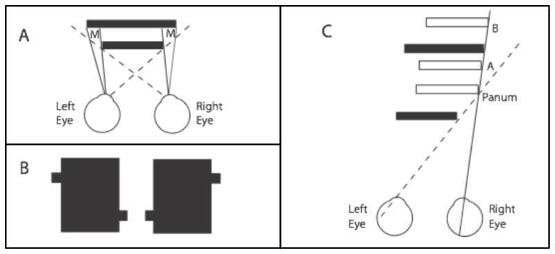
The geometry of occlusion and depth. A. Illustrates the case where one opaque rectangle positioned in front of another creates a monocular region M on the left for the left eye, and a similar monocular region M on the right for the right eye. B. This stereogram illustrates two partially occluded rectangles, one of which appears behind the large center rectangle, while the other appears in front and generates illusory contours. This clearly illustrates that depth is possible from occlusion. C. Depth ambiguity and constraint line under occlusion conditions. The solid front rectangle occludes the left eye's view of anything farther away than the dashed sight line. The right eye has an unoccluded view of the right edge of the rear solid rectangle along the solid sight line, but no depth information is available, so the rear black rectangle could lie anywhere along this sight line that is behind the left eye dashed occlusion line. Three possible locations are shown at A, B, and Panum. The latter is Panum s limiting case, the closest possible location of the occluded rectangle.

The first evidence that depth could be realized from occlusion was published by Gillam and Borsting (1988). They showed that the occluded and therefore unmatchable regions in RDSs actually hasten disparity processing and improve its accuracy. This happens, they reckoned, because unmatchable features generated by occlusion are actually a highly reliable signature of depth discontinuities at the edges of surfaces. Conversely, they argued that binocularly viewable features simply define internal aspects of an object s surface but not its boundaries.

This discovery led to questions concerning the accuracy of depth from occlusion. A key observation was that an object visible in only one eye due to occlusion could, in fact, lie anywhere along a depth constraint line, as depicted in Figure 2C (Nakayama & Shimojo, 1990). The binocularly visible, solid object depicted by the front black rectangle occludes the rear solid black object in the left eye view, as shown by the dashed sight line. However, the right eye view alone contains no geometric evidence to indicate whether the object edge is at the true depth as opposed to any of the other depths indicated by the white rectangles or indeed at any of an infinite number of other locations at or beyond that marked Panum (corresponding to Panum s limiting case). Because of its similarity to occlusion of background objects discussed by Leonardo da Vinci in the context of paintings, this was dubbed “da Vinci stereopsis” (Nakayama & Shimojo, 1990). Obviously, this depth ambiguity could lead naturally to very poor depth estimates for occluded objects. In many cases, of course, the occluded portion of the rear object is part of a much larger background that contains binocularly fusible features or textures beyond the occluded zone. When these binocular background textures are similar to the textures in the occlusion zone, the visual system interprets the occluded region as an extension of the background at the same disparity (Anderson & Nakayama, 1994). In cases such as that depicted in Figure 2A, however, there is no binocularly visible background, so this approach is impossible. Upon exploring this problem, Nakayama and Shimojo (1990) showed that as long as the occlusion zone was not more than about 15–30 arc min in extent, the occluded object was located near the smallest possible depth. Others subsequently noted that the smallest possible disparity of an occluded object corresponds to Panum s limiting case and ultimately provided evidence that occluded objects are seen at Panum s location when the evidence is consistent with this interpretation (Gillam et al., 2003; McKee et al., 1995; Liu et al., 1994). In this case, highly precise depth matching is possible. The key factor seems to be that the occluded object should include a line or edge parallel to the edge of the occluding surface. When the monocular stimuli are small disks rather than lines, however, the disk is perceived behind the occluding surface, but its depth is indeterminate and does not fit the Panum case (Gillam et al., 2003). Thus, apparently the Nakayama and Shimojo (1990) form of stereopsis from occlusion involves two different processes, depending on the nature of the occluded object.

A recently developed neural model for da Vinci stereopsis (Assee & Qian, 2007) comprises a simulated V1 stage providing inputs to a model V2 stage. The V1 stage utilizes both position and phase disparity energy units within a coarse-to-fine disparity computation, as described previously. Briefly, the model first uses very large receptive fields to make a crude position disparity estimate that then constrains phase disparity estimates on the next finer spatial scale. Both phase and position disparity are then estimated on this scale, and then the position disparity is passed on to the next finer disparity scale until the finest scale is reached. Cells in the simulated V2 layer then receive inputs from horizontally displaced V1 spatial arrays of units sensitive to different disparities. Accordingly, these V2 units provide the strongest responses when there is a disparity discontinuity, i.e. a depth-edge, present in the receptive field. Physiological evidence supports the presence of units sensitive to relative disparity and, therefore, disparity edges in V2 but not in V1 (Thomas et al., 2002; Cumming & Parker, 1999). Simulations show that this two-stage model accurately simulates Panum s limiting case and also can explain depth from monocular regions in da Vinci stereopsis. The reader is referred to the original paper for mathematical details of this sophisticated model. Anderson (2003) has also developed a computational model for depth from occlusion, although the model was not implemented as a neural network.

While on the topic of stereo from occlusion, we should mention second-order stereopsis, which represents the stereo extension of a number of second-order visual phenomena (Wilson, 1999). A second-order stimulus (sometimes termed non-Fourier) is defined by an internal texture (e.g., random dots, oriented bars, etc.) windowed by an envelope of significantly larger size than the texture elements. In the stereo case, the textures in the two monocular second-order stimuli cannot be fused, as they comprise orthogonal bars, independent random dot pattern or some other difference in feature space. Note that second order stereo stimuli can be regarded as an ecologically possible case of occlusion in which a surface in depth has window-shaped holes that constrain each eye to a very different view of a background at still greater depth. It has been shown that the envelopes can be fused to extract disparity information, although the accuracy is significantly lower than when the internal textures are fusible (Hess & Wilcox, 1994). Future work needs to link second-order stereopsis to theories of stereo from occlusion and, for that matter, to binocular rivalry.

Surfaces and Stereo

Twenty-five years ago stereopsis research tended to focus on stimuli containing just a few (often two) fronto-parallel surfaces at different depths. This was true of many studies using RDSs and also most work involving depth from occlusion. In the real world, however, many objects have curved surfaces (e.g., fruits and faces), meaning that local disparity structure varies smoothly (Koenderink, 1990). Accordingly, we have seen the emergence of interest in the perception of three-dimensional surface shape using non-planar disparity structures. Psychophysical evidence for the importance of local surface shape came from studies showing that stereoacuity and stereothresholds are, in fact, determined relative to the local 3D surface structure. We know this, for example, from measurements of increment thresholds measured relative to a 3D tilted plane (Glennerster et al. 2002) and of stereoacuity assessed on complex, curved 3D surfaces (Lappin & Craft, 2000). Moreover, smooth disparity interpolation is very effective on curved 3D surfaces as evidenced by excellent surface curvature identification even when curvature is specified by periodically sampled disparity values producing gaps up to 10 arc min in width (Yang & Blake, 1995).

Local 3D surface shape requires information about both local tilt and 3D curvature, defining how tilt changes between adjacent locations. Locally, left-right tilt can be conveyed by local interocular spatial frequency differences (Blakemore, 1970), while top-to-bottom tilt can be conveyed by interocular orientation differences (Ninio, 1985). Grossberg (1994) developed a model combining disparity with interocular spatial frequency and orientation differences to estimate 3D surface shape promoting figure-ground segregation. More recently, local 3D curvature along orthogonal axes has been emphasized by Lappin and Craft (2000) as a key determinant of surface shape. They provided psychophysical evidence supporting 3D surface curvature as an invariant in stereopsis but did not attempt to model the underlying neural computations necessary to support 3D curvature extraction. Such a model was developed by Li and Zucker (2010), with 3D curvature analysis based on interocular disparity, spatial frequency, and orientation differences. Computations showed this approach to be more accurate than previous models in extracting 3D curvature from stereograms of faces and scenes.

Recent research in primate electrophysiology has also contributed to our understanding of the representation of 3D surface structure in the brain. For example, Orban, Janssen and Vogels (2006) showed that a small sub-region of cortical area TE contains neurons sensitive to 3D surface curvature. A second area in caudal intraparietal cortex also contained neurons sensitive to 3D structures, but these were most strongly excited by depth orientation of surfaces and elongated objects. Thus, extraction of 3D surface shape occurs in higher visual cortical areas that build upon more elementary processing in lower areas beginning with V1 and V2. In addition, both the dorsal and ventral pathways are involved in processing 3D shape, albeit with different emphases and for different purposes (e.g. object recognition versus grasping or spatial navigation respectively).

Motion in depth

Regan pioneered work on this topic in his seminal experiments with Beverly (Regan & Beverley, 1973; Regan & Beverley, 1979; see Regan, 2000 for a review of his contributions). One early discovery was that changing disparity only produces a sensation of motion in depth when a cue for relative disparity is present (Regan et al., 1986). In 1993, Regan defined a key issue that turns out to be central to recent work on motion in depth. Specifically, motion in depth can be computed from the ratio of monocular velocities or it can be computed from the rate of change of disparity relative to a binocularly fixed object which provides a relative disparity reference (Regan, 1993). Cumming and Parker (1994) created stimuli that dissociate these cues, i.e., temporally uncorrelated RDSs, and compared threshold amplitudes for motion in depth with those obtained using RDSs that did contain monocular velocity information. Thresholds were somewhat better in the temporally uncorrelated case, suggesting that temporal change in disparity per se provides the signal for motion in depth, with monocular velocity ratios playing little or no role. Experiments from other laboratories using a variety of paradigms also support a major role for changing positional disparity in computations of motion in depth (Harris et al., 1998; Sumnall & Harris, 2002; Harris et al., 2008; Lages et al., 2003).

This conclusion has been challenged, however, by Shioiri et al. (2000) in a study showing that monocular velocities can be used to discriminate motion in depth. They used binocularly uncorrelated RD kinematograms with monocular images that were random with respect to one another. The stimuli contained just 2 frames in each eye, with 100% correlation over time within each monocular image. Translations were introduced in opposite directions between frames in the upper and lower half fields, so that monocular velocity differences would signal half of the pattern as moving forward and the other as receding. As no pair was fusible, there was no disparity, yet direction of motion in depth was discriminable for sufficiently high RD contrasts. These results were obtained even though rivalry was simultaneously perceived. The authors concluded that monocular velocity signals could be used in addition to temporal changes of disparity.

A subsequent study supported the use of monocular velocity signals for motion in depth processing using the motion aftereffect (Fernandez & Farell, 2006). Only one eye was adapted to motion of an RD kinematogram, thus eliminating any changing disparity signals. Tests with static binocular RDSs showed that motion in depth discrimination was almost perfect, indicating that interocular velocity difference aftereffects can generate motion in depth in the absence of any disparity.

Motion in depth processing has also been studied using fMRI. One study showed that motion in depth selectively activates a novel motion area adjacent and slightly anterior to (or partially overlapping) human MT+ (Likova & Tyler, 2007). A more recent study investigated the responses of human MT+ to both cues – velocity disparity and changing positional disparity -- to motion in depth (Rokers et al., 2009). A third fMRI study of motion in depth utilized a variant of the Pulfrich effect by presenting identical dynamic visual noise patterns to the two eyes, but with a slight temporal lag in one eye, which yielded a percept of a cylinder rotating in depth (Spang & Morgan, 2008). Relative to a non-delay condition, which produced no depth percept, the delay-induced depth percept produced more activation in the dorsal pathway including MT+ and intraparietal sulcus. Thus, brain imaging supports utilization of both cues in motion in depth computations and indicates the existence of an area adjacent to MT+ specialized for motion in depth. In this regard, it is noteworthy that neurons in macaque MT register disparity information as well as motion information (DeAngelis & Uka, 2003), with interactions between disparity and motion (Bradley et al., 1995).

The bulk of evidence implies that temporal changes in disparity provide the strongest input to computations of motion in depth, while monocular velocity ratios still provide useful information. It will be informative to learn whether a cue combination model can unify these alternative sources of information (Landy et al., 1995). Harris and colleagues have provided a contemporary view of the evidence on this issue (Harris et al., 2008). Indeed, unpublished data from the Harris lab suggests that individuals differ in the degree to which these two factors contribute to perception of motion in depth (Nefs et al., 2009). Future work likely will resolve this issue.

Although not strictly an instance of motion in depth, the kinetic depth effect also represents a situation where motion and depth signals are interrelated. For example, dots with appropriate velocities flowing in opposite directions in the same region of space can cause perception of, say, a rotating cylinder in which one set of dots appears behind the other, thus defining an apparent direction of cylinder rotation. Because the depth ordering is ambiguous, the perceived direction of rotation reverses haphazardly in a manner analogous to dominance switches in binocular rivalry. Nawrot and Blake (1991) proposed a model for this phenomenon in which there was disparity specific inhibition between dots moving in opposite directions. Adaptation of active units proved sufficient to produce reversals in the model analogous to those seen perceptually. The basic elements of this model were subsequently reported at the single unit level in macaque MT, where 40% of the units were found to be inhibited by motion in the opposite direction, but primarily at the same disparity (Bradley et al., 1995). These motion and disparity tuned interactions in MT would support the kinetic depth effect but could not explain motion in depth produced by temporal change of disparity. This is compatible with brain imaging evidence that motion in depth is largely processed in an area adjacent to human MT+ (Likova & Tyler, 2007).

Development of Stereopsis and the Existence of Critical Periods

Space constraints preclude our discussing developmental aspects of stereopsis in any detail. However, there is one dramatic, recent account implying stereoscopic plasticity in adulthood that deserves mention. As we all know, Hubel and Wiesel demonstrated the existence of a so-called “critical period” during which normal binocular inputs were necessary for normal development of cortical binocularity (Hubel & Wiesel, 1965). This conclusion was based, among other reasons, on induced strabismus in kittens. When done early in the kitten s life, induced strabismus produced wholesale loss in V1 binocular cortical cells, with those cells instead being activated by the non-deviating eye only. When these strabismic animals were studied as adults, this abnormal ocular dominance was still found. Hence, the prevailing wisdom dictated that a critical period of normal binocular input early in life was required for normal stereoscopic development to occur. Poor stereoscopic vision in people with strabismus dovetailed with this conclusion.

But then Oliver Sacks (2006) introduced us to “Stereo Sue” who, in fact, is neuroscientist Susan Barry. She has written a book describing the training and neural plasticity revealed as she slowly recovered from strabismus at birth followed by three corrective surgeries in her early youth (Barry, 2009). These surgeries cosmetically realigned her eye, but not sufficiently accurately for her to develop stereopsis. As an undergraduate at Wesleyan University, she took a neuroscience course that described critical periods and explained how her vision was different and why she would never perceive depth as other adults do. Curious as to why V1 binocular plasticity seemed to vanish at the end of the critical period, she located a group of developmental optometrists who studied and practiced the restoration of binocular vision through vision training, targeting children and adults (Griffin & Grisham, 2002). The result of several years of exercises to trigger her previously imperfectly aligned eyes to process the same region of space suddenly, at age 50, resulted in her seeing disparity produced depth for the first time. To quote her description of an early stereoscopic experience:

I rushed out of the classroom building to grab a quick lunch, and I was startled by my view of falling snow. The large wet flakes were floating about me in a graceful, three-dimensional dance. In the past, snowflakes appeared to fall in one plane slightly in front of me. Now I felt myself in the midst of the snowfall, among all the snowflakes. … I stood quite still, completely mesmerized by the enveloping snow. (Barry, 2009, p. 124)

When Barry contacted David Hubel, he was extremely supportive and encouraged her to continue her orthoptic treatments. In addition, he indicated that he and Torsten Wiesel had never tried to correct the strabismic deficits in their experimental animals, because it would have required difficult ocular re-alignment surgery and extremely difficult or impossible vision therapy training for the animals.

Many vision scientists, the authors included, used to accept a fairly rigid view of the critical period that downplays the success of orthoptics in treating strabismus. Clearly, adult visual plasticity in stereopsis is an area deserving of more future research, and it will require reconciling these remarkable clinical cases with experimental work showing that alternating monocular stimulation regimens by themselves are insufficient to restore normal stereopsis in animals raised with strabismus (Mitchell et al., 2009).

Future of Stereopsis Research

Several problem areas discussed above are ripe for major advances in the next few years. One is elucidation of the relative roles of position and phase disparities. There are currently sophisticated computational models based on very different perspectives, but more experimental data bearing on these issues are clearly needed. A more general problem area is the integration of 3D curved surface perception with depth edges indicated by occlusion. In natural scenes a foreground face or body is described by a 3D surface demarcated by depth edges that typically produce local background occlusion. Development of experimental paradigms to combine these multiple sources of stereoscopic depth information should aid enormously in the development of an integrated understanding of three-dimensional vision. Results from such studies should also provide revealing stimuli for fMRI studies designed to further differentiate stereo processing in dorsal and ventral streams.

On a practical note, the growing popularity of 3D movies such as “Avatar” and the advent of 3D television herald an enormous expansion of the role of stereopsis in our cultural life. We are going to witness development of powerful new technologies for presenting 3D static and moving visual stimuli, and these technologies will be of obvious benefit to vision science as tools for expanding our understanding of stereopsis.

In the next section we turn to what could be construed as the antithesis of stereopsis, i.e., binocular rivalry: stereopsis seemingly implies binocular cooperation whereas rivalry entails competition.

Binocular rivalry

The past twenty-five years have witnessed a surge of interest in binocular rivalry, as evidenced by the large number of publications dealing with the topic. Moreover, interest in rivalry spread beyond visual science into clinical psychiatry (Nagamine et al., 2009), gerontology (Norman et al., 2007), neurology (Bonneh et al., 2004; Valle-Inclan & Gallego, 2006), physics (Loxley & Robinson, 2009; Manousakis, 2009), human factors (Patterson et al., 2007), statistics (van der Ven et al., 2005) and philosophy (Cosmelli & Thompson, 2007). Reviews of contemporary work on rivalry can be found in several sources including an edited volume (Alais & Blake, 2005), review articles (Blake & Logothetis, 2002; Tong et al., 2006), chapters (Blake & O Shea, 2009) and the world-wide web (Scholarpedia and Wikipedia). The following sections highlight major themes that have emerged from this work.

What rivals during rivalry?

This simple question has generated controversy that, in turn, has produced a number of clever, revealing experiments. In the late 1980 s, the conventional view held that rivalry was eye-based, with competition transpiring between monocular neural representations of the two dissimilar stimuli. This idea came to be known as eye-based rivalry, although no one actually believed that one entire eye's view competed with the other. Rather, the consensus idea, embodied in several neural models of rivalry (e.g., Lehky, 1988; Blake, 1989), was that competition occurred between neurons representing local corresponding regions, i.e., zones, of the two eyes views. Still, eye-based rivalry was an appropriate characterization, for this conceptualization treated rivalry as a local process transpiring at an early stage of visual processing where eye-of-origin information was maintained within the neural elements representing the competing monocular stimuli. That view, incidentally, receives support from several more recent psychophysical papers showing that eye of origin information is importantly involved in aspects of rivalry (Shimojo & Nakayama, 1990; Ooi & He, 1999; Silver & Logothetis, 2007; Arnold et al., 2009; Bartels & Logothetis, in press). It also receives at least indirect support from human brain imaging studies showing modulations of neural responses within brain structures early in the visual hierarchy, including the thalamus (Wunderlich et al., 2005; Haynes et al., 2005) and monocular neurons in the V1 representation of the blind spot (Tong & Engel, 2001).

Two highly influential papers, both published in 1996, were construed as evidence undermining eye-based rivalry. In one of those papers, Kovács and colleagues (1996) devised “composite” rival targets consisting of fragments of two complex images, an example being the bottom pair shown in Figure 3a. With practice, observers can experience periods during which one image or the other is visible in its entirety. This outcome, referred to as interocular grouping (IOG), would be impossible, of course, if the left eye were competing with the right eye for dominance during rivalry.² Kovács et al. commented that the incidence of coherent perception was significantly less than that experienced with coherent, monocular images (upper pair of images in Figure 3a), and Lee and Blake (2004) showed how overall dominance with IOG could consist of patches, or zones, of dominance coordinated spatially between the two eyes. There is no doubt, however, that IOG reveals the operation of potent, synergistic influences governed by spatial coherence that promotes stimulus dominance during rivalry; this point is well documented in subsequent work inspired by Kovács et al s influential paper (Pearson & Clifford, 2005; Alais et al. 2006; Silver & Logothetis, 2007; Knapen et al., 2007).

Figure 3.

Panel a. Upper pair of figures are conventional rival stimuli, where separate, complete images are presented to the two eyes. Lower pair of figures are patch-wise rival stimuli that require interocular grouping in order for a coherent figure to be seen. (Figure reproduced with permission from Kovács et al, 1996. Copyright 1996, The National Academy of Sciences of the USA.). Panel b. Upper figure shows schematic of rapid eye-swap procedure used to induce stimulus rivalry. Rival targets are repetitively exchanged between the two eyes several times per second, with very rapid flicker used to mask transients associated with eye'swaps. Middle figure shows histograms of dominance durations measured without eye'swapping (left histogram) and with eye-swapping (right histogram). Lower figure summarizes the range of spatial and temporal frequencies yielding stimulus rivalry, measured using low and high contrast rival targets. (Figures in upper and lower panels reproduced with permission from Lee and Blake, 1999. Copyright 1999, Elsevier. Figure in middle panel reproduced with permission from Logothetis, Leopold and Sheinberg, 1996. Copyright Nature Press 1996.)

The other influential paper was published by Logothetis et al. (1996), who documented the existence of slow alternations in perceptual dominance between two orthogonally oriented gratings flashed at about 18 Hz and repetitively swapped between the two eyes approximately 3 times a second (Figure 3b). These periods of sustained dominance of one stimulus, in other words, transcended multiple swaps of the two rival stimuli between the eyes, implying that the rivalry triggered by these conditions did not involve competition between the two eyes. They dubbed this phenomenon stimulus rivalry and concluded that it constituted evidence against eye-based theories of binocular rivalry. This paper has been widely cited and, together with neurophysiological results from David Leopold s dissertation (Leopold & Logothetis, 1996), helped swing the pendulum of thought back to a high-level account of binocular rivalry advocated in the mid-20^th century (Walker, 1978).

A number of more recent findings, however, indicate that stimulus rivalry and conventional binocular rivalry are not strictly equivalent. For example, stimulus rivalry is confined to a narrower range of spatial and temporal frequencies compared to conventional rivalry (Lee & Blake, 1999; see Figure 3b), and stimulus rivalry and conventional rivalry differ in their dependence on stimulus size and contrast (Bonneh et al., 2001). Stimulus rivalry is more likely to be disrupted by brief blank periods occurring shortly after a transition in rival state whereas eye-based rivalry tends to be disrupted when swaps occur several seconds after a state transition (Bartels & Logothetis, in press). Similarly, the incidence of stimulus vs eye-based rivalry can be biased toward one or the other depending on how the dissimilar stimuli are tagged by contrast or temporal frequency (Silver & Logothetis, 2007). The emerging consensus is that eye-based rivalry and stimulus rivalry are distinct but related processes arising from neural events distributed over multiple stages of the visual hierarchy (Blake & Logothetis, 2002; Ooi & He, 2003; Wilson, 2003; Tong et al., 2006).

Whenever this hybrid conceptualization is referenced in today s literature, stimulus rivalry is always attributed to neural events transpiring at higher stages of cortical processing situated after inputs from the two eyes have been combined (e.g., Stuit et al., 2009). But given this conceptualization, one still must explain how dissimilar monocular stimuli rapidly swapped between the eyes escape interocular competition implicated in eye-based rivalry. Wilson (2003) developed a reciprocal inhibition model in which the conditions producing stimulus rivalry disengage inhibitory interactions in primary visual cortex, owing to the rapid temporal fluctuations typically associated with stimulus rivalry. Grossberg and colleagues (2008) employed a more complex circuitry to account for stimulus rivalry, but they, like Wilson, assumed that rapid stimulus flicker partially neutralizes neural processes (adaptation, in their case) that would ordinarily promote perception of rapid swapping and not stimulus rivalry. Both models treat stimulus rivalry as a default outcome when mechanisms engaged by conventional rival stimulation are disengaged.

It is safe to predict that the issue of eye vs stimulus rivalry will continue to attract interest, with the focus shifting to integration of the two views rather than arguments about which view is correct.

What triggers alternations during rivalry?

Several intriguing hypotheses have been advanced to explain the transitions inherent in rivalry. The conventional explanation, embodied in several models, identifies neural adaptation as the key ingredient in the alternation process. On this view, neural activity associated with the currently dominant stimulus wanes over time, eventually reversing the balance of activity between the two neural representations and, hence, triggering a switch in perceptual dominance (e.g., Lehky, 1988). This hypothesis readily comports with both stimulus-based and eye-based accounts of rivalry, for the putative adaptation process that differentially modulates the effectiveness of neural representations could arise anywhere within the visual pathways (e.g., Lago-Fernández & Deco, 2002). Moreover, several lines of evidence are consistent with adaptation s involvement in alternations (Blake et al., 2003; Carter & Cavanagh, 2007; Alais et al., in press). Adaptation alone, however, cannot fully account for the dynamics of binocular rivalry (Brascamp et al., 2006; Kim et al., 2006; Suzuki & Grabowecky, 2007) nor for the long-term sequential dependence of state durations (Gao et al., 2006). Neither can adaptation easily explain the influence of emotional connotation (e.g., Alpers & Pauli, 2006) and bisensory interactions (e.g., Lunghi et al, 2010) on those dynamics.

To remedy the shortcomings of adaptation-based rivalry alternations, several models have incorporated neural noise (either in the inhibitory network or in the excitatory signals representing the rival stimuli) to account for the stochastic properties of successive rivalry states (Kalarickal & Marshall, 2000; Laing & Chow, 2002; van Ee, 2009). It is unlikely, however, that noise alone will reproduce all the dynamical behaviors exhibited during rivalry, implying that successful neural models of rivalry will need to incorporate both adaptation and noise (e.g., Shpiro et al., 2009). We can also expect to see growing interest in the possible relation of binocular rivalry to the concepts of attractor states embodied in physical systems, such as double-well potential framework applied to binocular vision decades ago by Sperling (1970) and elaborated more recently within the context of rivalry (Wilson, 1999; Kim et al., 2006; Moreno-Bote et al., 2007). The coming years will no doubt see movement in that direction, but those modeling efforts must eventually be grounded in neurophysiology for them to make contact with the bulk of theoretical work on rivalry (Rubin, 2003). Moreover, this theoretical work needs to be complemented by fMRI and VER studies identifying neural concomitants of noise and neural adaptation. Finally, the role of noise in rivalry alternations may be more fruitfully conceptualized within the framework of unexplained error variance, not simply random fluctuations in signal quality, a point we revisit later in this section.

A substantially different hypothesis about the basis of rivalry alternations was proposed by Pettigrew (2001). According to his view, clock-like, neural oscillators control perceptual alternations in rivalry and, for that matter, alternations during other forms of perceptual bistability. Pettigrew speculates that these oscillators reside in subcortical structures and separately drive the two hemispheres of the brain. Suggestive evidence for these putative oscillators includes the positive correlation in alternation rates for different forms of perceptual multi-stability among individuals (Carter & Pettigrew, 2003). Pettigrew and colleagues think that these oscillators are susceptible to fluctuations in serotonin levels, governed either endogenously (Miller et al., 2003) or exogenously (Carter et al., 2005), in which case this hypothesis could potentially be relevant to medical conditions such as schizophrenia and bipolar disorder (Pettigrew & Miller, 1998) with a likely genetic component (Miller et al., 2010). This possibility has been questioned, however, by other studies of bistable switch rates in bipolar disorder (Krug et al., 2008). Moreover, the theory that an oscillator creates rivalry alternations separately in the two hemispheres does not comport with the findings of O’Shea and Corballis (2003) that rivalry alternations in split-brain patients are equivalent to those in normal observers (see also O’Shea & Corballis, 2005). The idea of a central oscillator also leaves unexplained key aspects of binocular rivalry, including its tendency to follow specific phase-space trajectories (Suzuki & Grabowecky, 2002), the vast difference in temporal period between hemispheric oscillations and dominance periods, and the strong tendency for initial dominance to vary idiosyncratically within the visual field (Carter & Cavanagh, 2007). In general, this provocative idea requires further refinement to address important characteristics of rivalry by which other models are usually judged.

A third, recent idea about rivalry alternations ascribes them to the brain s putative propensity to continuously reevaluate perceptual interpretations of sensory information (Leopold & Logothetis, 1999; Sterzer et al., 2009). This idea, grounded in the view that perception is an inference-like process, has been formalized in several models of rivalry, including one in which predictive coding is developed within a Bayesian framework (Hohwy et al., 2008; see Dayan, 1998, van Ee et al., 2003, and Wilson, 2009 for related instantiations of inference-based accounts of rivalry). These conceptualizations based on predictive coding have the virtue of integrating the roles of top-down and bottom-up processes (Tong et al., 2006) within a unifying mechanism that comprehensively captures a wide range of dynamical properties of rivalry. Moreover, models based on predictive coding can account for the frontal cortical activations associated with transition states during rivalry measured using fMRI (Lumer et al., 1998): according to predictive coding, those transition periods are occasioned by heightened uncertainty (i.e., temporarily large error variance) about which of several alternative perceptual interpretations is currently most likely (Knapen et al., 2008). It is noteworthy, too, that the predictive coding view of rivalry is not necessarily incompatible with the involvement of adaptation and noise in promotion of alternations, for those processes could be intrinsic to the inference process. Thus, for example, “noise” in the model advanced by Hohwy et al. (2008) would correspond to unexplained prediction error, not random fluctuations in activity associated with competing neural representations.

Two documented influences on binocular rivalry dynamics have a cognitive flavor to them. One of those influences is attention, which can bias initial dominance at the onset of rival stimulation (Mitchell et al., 2004; Chong & Blake, 2006) and lengthen subsequent durations of dominance as rivalry continues (Ooi & He, 1999; Chong et al., 2005). Attention is not omnipotent, however, for it cannot arrest alternations in rivalry (Meng & Tong, 2004). Nor is attention essential for alternations occur when attention is diverted (Paffen et al., 2006). The second cognitive-like influence in binocular rivalry is a form of perceptual memory created when rival stimulation is presented intermittently: insertion of short blank periods tends to stabilize dominance of a given stimulus over durations an order of magnitude longer than dominance durations experienced during uninterrupted rival stimulation (Leopold et al., 2002). Pearson and Brascamp (2008) detail how to promote this form of perceptual memory, and Wilson (2007) and Noest et al. (2007) offer models of rivalry aimed at accounting for it.

Any successful model of binocular rivalry alternations must explain not only the temporal sequence of alternations but also several spatial properties characteristic of rivalry transitions. It is widely known, for example, that transitions in dominance do not occur instantaneously but, instead, tend to arise within a localized area of a previously suppressed rival figure and then spread quickly throughout the rest of that figure. The spatial location where changes in rival state originate can be biased by stimulus manipulations (Paffen et al., 2008), and the point in time at which a transition occurs can be triggered by increments in the contrast of a currently suppressed rival stimulus (Blake et al., 1990). In fact, with appropriately configured rival stimuli, these transitions can appear as traveling waves of dominance whose origin can be controlled, whose spread can be channeled and speed can be measured (Wilson et al., 2001; Kang et al., 2009) and whose neural correlates can be identified using fMRI (Lee et al., 2005).

What survives binocular rivalry suppression?

When a stimulus succumbs to suppression during rivalry, its disappearance can perceptually resemble the physical removal of that stimulus. But does such a stimulus retain any of its effectiveness despite being suppressed from awareness? And, if so, what aspects of a suppressed stimulus are still registered despite the phenomenal disappearance of the stimulus? In recent years, a number of studies have asked versions of these questions, and the results point to wide-ranging dissociations between perceptual invisibility and neural effectiveness. We know, for example, that suppressed stimuli can induce adaptation aftereffects thought to arise at relatively early stages of visual processing (see review by Blake & He, 2005). Originally it was concluded that the survival of adaptation aftereffects induced during suppression implied that the neural events underlying suppression transpired after the neural site where those aftereffects originated. However, that conclusion has been tempered by the realization that aftereffects, while not abolished by suppression, may be reduced in strength, implying that neural activity associated with a suppressed stimulus has been attenuated but not abolished (Blake et al., 2006). Neural adaptation believed to transpire at higher levels within the visual hierarchy (e.g., ventral stream areas involved in face processing), in contrast, appears to be completely blocked when the adaptation stimulus (e.g., a face) is suppressed from awareness³ (Moradi et al., 2005; see van der Zwan et al., 1993, for the same pattern of results in the case of optic flow).

In addition to the survival of adaptation aftereffects induced during suppression, other lines of evidence reveal residual effectiveness of a stimulus suppressed during rivalry. For instance, pictures of manipulable objects rendered invisible by suppression nonetheless can produce visual priming as evidenced by speeded reaction times on a categorization task (Almeida et al., 2008). In a similar vein, pictures of arousing stimuli (e.g., nude individuals) can covertly guide visual attention to the location of that picture even when the picture is suppressed from awareness during rivalry (Jiang et al., 2006). For that matter, a suppressed stimulus can influence the perceptual appearance of the currently dominant stimulus, causing a change in its perceived orientation (Pearson & Clifford, 2005), its perceived direction of motion (Andrews & Blakemore, 2002) or its perceived color (Hong & Shevell, 2009). Also indicative of residual neural effectiveness of a suppressed stimulus are studies showing that the duration of suppression of a stimulus is abbreviated when that stimulus conveys meaningful or emotionally charged information (Jiang et al., 2007; Yang et al., 2007) or when the observer s own actions unknowingly control the motion of that suppressed stimulus (Maruya et al., 2007). Finally, there are studies showing that a suppressed stimulus can contribute to stereoscopic depth perception, a point we revisit below.

The same question– to what extent does a suppressed stimulus remain effective during rivalry –has also been tackled using fMRI. Here the strategy has been to ask whether the magnitude of the BOLD signal evoked by a rival stimulus depends on the perceptual status of that stimulus, i.e., whether BOLD signals wax and wane in synchrony with rivalry alternations. The answer is “yes”–BOLD signals evoked by a rival stimulus are reduced in amplitude relative to signals produced when that stimulus is dominant (Figure 4a).

Figure 4.

Panel a. Modulations in BOLD signal are correlated with reversals in rivalry state. Upper figure shows BOLD signals during dominance and suppression phases of binocular rivalry measured in human lateral geniculate nucleus in response to a high contrast pattern viewed by one eye and a low contrast pattern viewed by the other eye. Signals are time locked to transitions in perceptual state as indicated by observers perceptual tracking records. Graph on the left shows BOLD modulations before and immediately following transitions in rivalry state between the two rival patterns; graph on the right shows BOLD modulations before and immediately following physical removal and presentation of the two patterns that mimic alternations of rivalry. Middle figure shows the same as top figure, except that BOLD signals are being measured within voxels retinotopically localized within visual area V1. Lower figure shows BOLD signals from two ventral stream areas selectively responsive to pictures of faces (fusiform face area: FFA) and pictures of houses (parahippocampal place area: PPA). Graph on the left shows changes in BOLD signals time-locked to transitions in rivalry dominance from the house to the face; graph on the right shows changes in BOLD signal time-locked to transitions in rivalry dominance from the face to the house. (Top and middle figures in a reproduced with permission from Wunderlich et al., 2005. Copyright 2005, Nature Press. Bottom figure reproduced with permission from Tong et al. 1998. Copyright 1998, Cell Press.) Panel b. Modulations in visual-evoked potentials (VEP, upper figure) and action potentials from individual neurons in the temporal lobe (lower figure) recorded from human observers experiencing binocular rivalry. (Upper figure reproduced with permission from Brown and Norcia, 1997. Copyright Elsevier, 1997. Lower figure reproduced with permission from Kreiman et al., 2002. Copyright 2002, The National Academy of Sciences of the USA).

Remarkably, those transient reductions are observed within very early stages of the visual pathway, including the lateral geniculate nucleus (Wunderlich et al., 2005; Haynes et al., 2005) and primary visual cortex (Polonsky et al., 2000; Tong & Engel, 2001; Lee & Blake, 2002). Moreover, the time course of BOLD signal modulations within the retinotopic map in V1 matches the observer s perceptual experience of spreading waves of dominance during state transitions in rivalry (Lee et al., 2005, 2007). BOLD signals associated with suppression phases are also strongly attenuated in higher tier visual areas, particularly within the ventral stream pathway (Tong et al., 1998; Moutoussis & Zeki, 2002; Moutossis et al., 2005; Jiang & He, 2006). It appears that neural concomitants of binocular rivalry suppression as indexed by BOLD signal modulations are more pronounced within ventral stream structures compared to the dorsal stream structures, at least for certain categories of objects (Fang & He, 2005). At the same time, fine-scale analyses of reduced amplitude BOLD signals in at least some of these ventral areas reveal the presence of residual, category-specific patterns of activation (Sterzer et al., 2009). Finally, several studies report the existence of robust, visually evoked BOLD signals in the amygdala even when the stimuli evoking those signals –faces portraying emotional expressions – are completely suppressed from awareness (Pasley et al., 2004; Williams et al., 2004; Jiang & He, 2006).

The BOLD signal, of course, reflects metabolic markers of neural activity, including neural responses other than action potentials (e.g., Logothetis, 2003). For this reason questions arise about the specific neural events underlying modulations in BOLD signals measured during binocular rivalry. Fortunately, other techniques are also available for measuring neural responses from the human brain, including some thought to originate from action potentials. Two of these brain imaging techniques, visual evoked responses (Brown & Norcia, 1997; de Labra & Valle-Inclán, 2001; Roeber & Schröger, 2004) and magnetoencephalography (Tononi et al., 1998; Srinivasan & Petrovic, 2006), have disclosed robust, rivalry-related fluctuations in signal strength (e.g., Figure 4b). But because of their coarser spatial resolution, VER and MEG do not pinpoint brain areas in which those modulations arise with the same precision as fMRI. A rare opportunity to measure action potentials from neurons in humans experiencing rivalry was exploited by Kreiman et al. (2002), who found reduced responsiveness measured with electrodes implanted in the medial temporal lobe of epilepsy patients exposed to binocular rivalry (see Figure 4b).

Considered together, these various studies suggest that the perceptual invisibility of a stimulus during rivalry is the culmination of a cascade of neural events transpiring within a hierarchy of visual stages. Some think that the depth of suppression grows as one ascends the hierarchy, as suggested by psychophysical results from test probe experiments (Alais & Melcher, 2007; Nguyen et al., 2003) and by single-cell recording results from awake, behaving monkeys experiencing binocular rivalry (Leopold & Logothetis, 1996). Today, multistage models of rivalry (Wilson, 2003; Freeman, 2005; Grossberg et al., 2008; Hohwy et al., 2008) have supplanted earlier models that treated rivalry as a winner-take-all competition occurring within a single stage (e.g., Blake, 1989). Studies dealing with residual effectiveness of a suppressed stimulus have been, and will continue to be, highly relevant in shaping our thinking about the nature and locus of neural mechanisms mediating rivalry. Indeed, rivalry suppression, because of its effectiveness in dissociating physical stimulation and visual awareness, has been touted as one of the paramount tools for identifying the neural correlates of consciousness (Koch, 2007). Kim and Blake (2005) detailed the advantages of rivalry over other techniques (e.g., masking) for manipulating conscious awareness, and Lin and He (2009) spelled out the rationale for using rivalry to study the neural concomitants of awareness.

To end this section on a practical note, the unpredictability of suppression phase durations, while interesting from the standpoint of neural dynamics, is a nuisance when one needs to maintain a stimulus in the suppressed state for a relatively long period of time. Several techniques have been devised to stabilize perceptual states during rivalry. One involves continuously moving rival stimuli around the visual field, with fixation maintained at a central point (Blake et al., 2003); this maneuver promotes long dominance durations, presumably by minimizing local neural adaptation. It is also possible to identify regions in the visual field where one rival stimulus reliably achieves initial dominance at the onset of rival stimulation (Carter & Cavanagh, 2007), providing another means for stabilizing perceptual dominance and, hence, suppression. These local regions of biased onset dominance remain stable for weeks or longer, but they are idiosyncratic across observers. Another technique for promoting reliable dominance, termed continuous flash suppression (CFS), presents to one eye a series of different, contour-rich patterns rapidly and sequentially flashed to one eye (Tsuchiya & Koch, 2005). An ordinarily conspicuous stimulus (e.g., the picture of a fearful face) pitted against CFS in the other eye can be completely suppressed for durations lasting a minute or longer. Another effective suppression technique, termed binocular switch suppression, swaps two rival stimuli of unequal stimulus strength repetitively between the eyes (1 Hz swap rate works fine), the result being that the stronger of the two stimuli remains visible continuously for up to 30 sec or longer (Arnold et al., 2008). Finally, as mentioned earlier, spontaneous fluctuations in rival state can be minimized by presenting rival stimulation intermittently, a maneuver that tends to stabilize the dominance of a given stimulus, albeit not indefinitely (Brascamp et al., 2009).

Relation of stereopsis and rivalry

It has long been known that rivalry and stereopsis can be experienced simultaneously (e.g., Treisman, 1962), and several recent papers have reconfirmed this striking observation using novel displays (e.g., Su et al., 2009). Yet there are situations where rivalry perturbs, or even destroys, stereopsis, indicating that the two processes are not independent. For instance, the quality of stereopsis in the presence of rivalry depends on the contrast of the two half-images, with stereopsis dominating when contrast levels are low and rivalry dominating when contrast is high (Blake et al., 1991). Stereopsis is also degraded when the two eyes view reverse contrast half-images and is abolished if those half-images are random-dot stereograms (e.g., Cogan et al., 1995). Rival stimulation is also more likely to perturb stereopsis when the spatial frequency and orientation content of the two half-images is similar (Buckthought & Wilson, 2007), a finding echoing earlier work by Julesz and Miller (1975).

Stereopsis and implied depth relations can also affect the incidence of binocular rivalry. For instance, depth implied by differential blur of two dissimilar monocular images can bias rivalry dominance in favor of the putatively nearer, more sharply focused image (Arnold et al., 2007). Even more compelling is the absence of rivalry when dissimilar monocular stimulation arises consequent to partial occlusion of a far surface by a nearer object (depth occlusion described in the section on stereopsis). In this situation, unpaired regions consistent with occlusion are assigned to an appropriate rear depth, whereas unpaired regions that violate occlusion lead to rivalry alternations (Shimojo & Nakayama, 1990). These findings have been formalized in an ambitious model that integrates stereopsis, partial surface occlusion and binocular rivalry, with a key ingredient in this model being interocular inhibition between neural representations of monocular surfaces that do not have matching representations in the other eye's view (Hayashi et al., 2004). This model echoes earlier suggestions that rivalry is the default outcome when binocular matching fails (e.g., Blake & Boothroyd, 1985) and it does so within a highly realistic context based on the geometry of binocular viewing. As discussed in an earlier section of this essay, a complementary version of this matching problem arises in situations where the number of potential binocular matches between left- and right-eye features far exceeds the actual matches implied by stable perception of surface structure in complex stereograms. Interocular inhibition is one means for eliminating false matches in those kinds of viewing situations (Marr & Poggio, 1976), and it is tempting to hypothesize that this inhibition is also involved in binocular rivalry. If that were true, results from physiological studies using anticorrelated RDSs could also shed light on the neural events underlying rivalry suppression (Cumming & Parker, 2000; Tanabe et al., 2004).

Binocular contrast summation

Binocular viewing is superior to monocular when it comes to threshold tasks such as contrast detection, a superiority generally called binocular summation. Twenty-five years ago, there were two alternative accounts of binocular summation, both aimed at describing what was then believed to be the ubiquitous 40% (i.e., ~ √2) summation ratio between monocular and binocular thresholds. One account posited linear summation of monocular contrast signals whose variances (“noise”) were uncorrelated (Campbell & Green, 1965); the other proposed that summation occurred between monocular signals passed through a non-linear transducer that squared those monocular signals prior to combination (Legge, 1984). Both of these accounts of binocular summation constitute single channel models (i.e., they ignore ocular dominance), and subsequent evidence (Anderson & Movshon, 1989) showed that a single-channel model was inadequate to account for contrast detection performance in the presence of noise and contrast detection under conditions of adaptation. Moreover, other studies have consistently found summation ratios in excess of √2, further undermining those original, single-channel models (e.g., Meese et al. 2006). In recent years, the field has come to appreciate that an adequate model of binocular combination needs to include dynamic contrast gain control, not just a static non-linear transducer and has come to accept that such a model must also account for dichoptic masking with its characteristic “dipper” shape as a function of contrast (e.g., Meese et al., 2006). The evidence moving the field in those directions has come largely from experiments that have measured contrast summation at threshold and suprathreshold levels and contrast masking using dichoptically presented grating patterns, often briefly presented.

During the past few decades, at least half a dozen models have been developed that go well beyond quadratic summation in their accounts of binocular combination (e.g, Cogan, 1987). We do not have the space to describe and differentiate these various models, nor to describe the psychophysical evidence motivating their architectures. Still, to provide some gist of the directions these models are evolving, we have selected two to highlight (see Figure 5).

Figure 5.

Multistage models of binocular contrast summation. a. Ding and Sperling model consisting of two pairs of contrast gain control mechanisms, with each pair linked in reciprocal inhibition. The earlier stage gain control is governed by the total weighted contrast energy (TCE) and the later stage gain control is selective for orientation and spatial frequency. b. Two-stage model published by Baker and Meese (2007). It comprises contrast gain control (divisive suppression) on separate orientation-selective monocular channels followed by phase-dependent binocular interactions of left- and right-eye channels (both in-phase and anti-phase components).

The model in Figure 5a, published by Ding and Sperling (2006), comprises initial left- and right-eye channels each receiving images I_L and I_R, respectively, with each channel containing two gain control mechanisms: a gain control mechanism non-selective for orientation and spatial-frequency (TCE: total weighted contrast energy) and a gain control mechanism selective for orientation and spatial frequency. The two TCE components exert reciprocal inhibition on one another in proportion to their respective TCE outputs [(ε_L(I_L) and (ε_R(I_R)], and the outputs of those TCE components [(ε_L(I_L)/(1+ε_R(I_R)) and (ε_R(I_R)/(1+ε_L(I_L))] exert gain control on the other eye's selective gain control. Outputs are summed binocularly to determine the magnitude of the binocular signal. The evidence in support of this architecture came from psychophysical measurements of perceived phase of a binocularly seen grating comprising the two monocular gratings that could differ in phase and contrast. (The gratings were oriented horizontally and did not, therefore, generate stereoscopic depth, only a perceived phase that varied with the balance between the two monocular contrasts.) The model makes the counterintuitive prediction that addition of noise to one eye's view should increase the relative effectiveness of that eye's grating (through that channel's TCE), a prediction that was indeed confirmed. At very short exposure durations, psychophysically measured contrast summation (as evidenced by perceived binocular phase) was linear, contrary to the model s predictions. But including a bandpass temporal filter in the gain control pathway was sufficient to accommodate the duration dependence of contrast summation. The model was also shown to account for perceived binocular contrast when the two eyes receive different contrast values. Ding and Sperling acknowledge that their 2006 model is designed to deal with situations where the two eyes receive compatible monocular stimuli and does not directly pertain to conditions provoking binocular rivalry.

An alternative model developed by the research group at Aston University, U.K. (e.g., Meese et al. 2006) is shown schematically in Figure 5b. Here, too, contrast gain control is applied at multiple stages, this time within monocular channels as well as at a site following binocular combination. In this model, the exponents governing gain control at the monocular levels were set sufficiently low to predict summation ratios in excess of √2, but the exponent at the binocular stage was set at a higher value to accommodate the “dipper” region characteristic of dichoptic masking functions at relatively low contrasts. In recent refinements of this 2-stage model, its authors have distinguished two mechanisms within each monocular gain control component, one mechanism that exerts a suppressive influence on contrast signals within the contralateral eye and a second mechanism that exerts suppression on its own eye's contrast signals. The mechanisms operating prior to binocular combination include suppression that is non-selective (or very broadly tuned) for orientation (along the lines of cross-orientation suppression identified physiologically, e.g. Bonds, 1989); further orientation- and phase-specific suppression may also occur before or after binocular combination. Also transpiring after binocular combination is a linear summation stage where contrast signals are pooled over space (Meese & Summers, 2009; see also Mansouri et al., 2005). The model emerging from this work differs from the Ding and Sperling model in several ways: 1) it posits ipsilateral suppression (which, according to the authors, could transpire at the level of the LGN), 2) it introduces a winner-take-all operator across monocular and binocular channels that governs performance without necessarily providing explicit information about which channel produced the response triggering that operator (i.e., an observer might be unable to judge whether a detection event is associated with monocular or binocular stimulation). This model has not been applied to the perceived binocular phase results of Ding and Sperling, and it remains to be determined whether the Ding and Sperling paper can account for summation in excess of √2 and the dipper portion of the dichoptic masking function (cf. Baker & Meese, 2007). That said, both models deftly account for the simple observation that the visual appearance of things hardly changes when one closes an eye (disregarding, of course, the loss of stereopsis), and both models have the ingredients necessary to promote competition when the two eyes view starkly different images (i.e., the stimulus conditions producing rivalry).

Finally, we have seen closer linkages established between these models and neurophysiological data on dichoptic visual masking (Macknik & Martinez-Conde, 2004), cross-orientation suppression (Freeman et al., 2002; Li et al. 2005; Sengpiel & Vorobyov, 2005) and contrast gain control (Truchard et al., 2000; Moradi & Heeger, 2009), not to mention connections to clinical conditions including strabismus (Baker et al., 2008). At the same time, these models of binocular contrast summation need to be expanded to account for the effect of chromatic contrast on binocular combination, for it is quite obvious that stereoscopic vision behaves differently when confronted with isoluminant half-images (e.g., Simmons & Kingdom, 1995).

Final Comments

The last quarter-century has witnessed stimulating controversies producing exciting advances in the field of binocular vision. As predicted 25 years ago by Bishop and Pettigrew (1986), those advances were sponsored by interactions involving psychophysics, neuroscience and computational modeling. It is safe to assume that this potent coalition in conjunction with newer brain imaging will continue to drive the field, but we cannot guess what highlights will be contained in the next anniversary essay in 2035. It has been said that the best way to predict the future is to create it, a job that now falls to today s students of binocular vision.

References

- Adelson EH, Bergen JR. Spatiotemporal energy models for the perception of motion. Journal of the Optical Society of America, A. 1985;2:284–299. doi: 10.1364/josaa.2.000284. [DOI] [PubMed] [Google Scholar]
- Alais D, Blake R. Binocular rivalry and perceptual ambiguity. Boston: MIT Press; 2005. [Google Scholar]
- Alais D, Cass J, O’Shea RP, Blake R. Visual sensitivity underlying changes in visual consciousness. Current Biology. 2010;20:1362–1367. doi: 10.1016/j.cub.2010.06.015. [DOI] [PMC free article] [PubMed] [Google Scholar]
- Alais D, Lorenceau J, Arrighi R, Cass JR. Contour interactions between pairs of Gabors engaged in binocular rivalry reveal a map of the association field. Vision Research. 2006;46:1473–1487. doi: 10.1016/j.visres.2005.09.029. [DOI] [PubMed] [Google Scholar]
- Alais D, Melcher D. Strength and coherence of binocular rivalry depends on shared stimulus complexity. Vision Research. 2007;47:269–279. doi: 10.1016/j.visres.2006.09.003. [DOI] [PubMed] [Google Scholar]
- Alais D, O'Shea RP, Mesana-Alais C, Wilson IG. On binocular alternation. Perception. 2000;29:1437–1445. doi: 10.1068/p3017. [DOI] [PubMed] [Google Scholar]
- Almeida J, Mahon BZ, Nakayama K, Caramazza A. Unconscious processing dissociates along categorical lines. Proceedings of the National Academy of Sciences of the United States of America. 2008;105:15214–15218. doi: 10.1073/pnas.0805867105. [DOI] [PMC free article] [PubMed] [Google Scholar]
- Alpers GW, Pauli P. Emotional pictures predominate in binocular rivalry. Cognition and Emotion. 2006;20:596–607. [Google Scholar]
- Anderson BL. The role of occlusion in the perception of depth, lightness, and opacity. Psychological Review. 2003;110:785–801. doi: 10.1037/0033-295X.110.4.785. [DOI] [PubMed] [Google Scholar]
- Anderson BL, Nakayama K. Towards a general theory of stereopsis: Binocular matching, occluding contours, and fusion. Psychological Review. 1994;101:414–445. doi: 10.1037/0033-295x.101.3.414. [DOI] [PubMed] [Google Scholar]
- Anderson PA, Movshon JA. Binocular combination of contrast signals. Vision Research. 1989;29(9):1115–1132. doi: 10.1016/0042-6989(89)90060-6. [DOI] [PubMed] [Google Scholar]
- Andrews TJ, Blakemore C. Integration of motion information during binocular rivalry. Vision Research. 2002;42:301–309. doi: 10.1016/s0042-6989(01)00286-3. [DOI] [PubMed] [Google Scholar]
- Arnold DH, Grove PM, Wallis TSA. Staying focused: a functional account of perceptual suppression during binocular rivalry. Journal of Vision. 2007;7:1–8. doi: 10.1167/7.7.7. [DOI] [PubMed] [Google Scholar]
- Arnold DH, Law P, Wallis TSA. Binocular switch suppression: A new method for persistently rendering the visible invisible. Vision Research. 2008;48:994–1001. doi: 10.1016/j.visres.2008.01.020. [DOI] [PubMed] [Google Scholar]
- Arnold DH, James B, Roseboom W. Binocular rivalry: Spreading dominance through complex images. Journal of Vision. 2009;9:1–9. doi: 10.1167/9.13.4. [DOI] [PubMed] [Google Scholar]
- Assee A, Qian N. Solving daVinci stereopsis with depth-edge-selective V2 cells. Vision Research. 2007;47:2585–2602. doi: 10.1016/j.visres.2007.07.003. [DOI] [PMC free article] [PubMed] [Google Scholar]
- Baker DH, Meese TS. Binocular contrast interactions: Dichoptic masking is not a single process. Vision Research. 2007;47:3096–3107. doi: 10.1016/j.visres.2007.08.013. [DOI] [PubMed] [Google Scholar]
- Baker DH, Meese TS, Hess RF. Contrast masking in strabismic amblyopia: Attenuation, noise, interocular suppression and binocular summation. Vision Research. 2008;48:1625–1640. doi: 10.1016/j.visres.2008.04.017. [DOI] [PubMed] [Google Scholar]
- Barry SR. Fixing My Gaze: a Scientist's Journey into Seeing in Three Dimensions. New York: Basic Books; 2009. [Google Scholar]
- Bartels A, Logothetis N. Binocular rivalry: a time-dependence of eye and stimulus contributions. Journal of Vision. doi: 10.1167/10.12.3. in press. [DOI] [PubMed] [Google Scholar]
- Bishop PO, Pettigrew JD. Neural mechanisms of binocular vision. Vision Research. 1986;26:1587–1600. doi: 10.1016/0042-6989(86)90177-x. [DOI] [PubMed] [Google Scholar]
- Blake R. A neural theory of binocular rivalry. Psychological Review. 1989;96:145–167. doi: 10.1037/0033-295x.96.1.145. [DOI] [PubMed] [Google Scholar]
- Blake R, Boothroyd K. The precedence of binocular fusion over binocular rivalry. Perception & Psychophysics. 1985;37:114–124. doi: 10.3758/bf03202845. [DOI] [PubMed] [Google Scholar]
- Blake R, He S. Visual adaptation as a tool for studying the neural correlates of conscious visual awareness. In: Clifford C, Rhodes G, editors. Fitting the mind to the world. Oxford University Press; 2005. pp. 281–307. [Google Scholar]
- Blake R, Logothetis NK. Visual competition. Nature Reviews Neuroscience. 2002;3:13–23. doi: 10.1038/nrn701. [DOI] [PubMed] [Google Scholar]
- Blake R, O’Shea RP. Binocular rivalry. In: Squire L, editor. Encyclopedia of Neuroscience. Vol. 2. Academic Press; Oxford UK: 2009. pp. 179–187. [Google Scholar]
- Blake R, Sobel K, Gilroy LA. Visual motion retards alternations between conflicting perceptual interpretations. Neuron. 2003;39:869–878. doi: 10.1016/s0896-6273(03)00495-1. [DOI] [PubMed] [Google Scholar]
- Blake R, Westendorf D, Fox R. Temporal perturbations of binocular rivalry. Perception & Psychophysics. 1990;48:593–602. doi: 10.3758/bf03211605. [DOI] [PubMed] [Google Scholar]
- Blake R, Yang Y, Wilson HR. On the coexistence of stereopsis and binocular rivalry. Vision Research. 1991;31:1191–1204. doi: 10.1016/0042-6989(91)90044-6. [DOI] [PubMed] [Google Scholar]
- Blake R, Tadin D, Sobel K, Chong SC, Raissian R. Strength of early visual adaptation depends on visual awareness. Proceedings of the National Academy of Sciences, USA. 2006;103:4783–4788. doi: 10.1073/pnas.0509634103. [DOI] [PMC free article] [PubMed] [Google Scholar]
- Blakemore C. A new kind of stereoscopic vision. Vision Res. 1970;10:1181–1199. doi: 10.1016/0042-6989(70)90036-2. [DOI] [PubMed] [Google Scholar]
- Bonds AB. Role of inhibition in the specification of orientation selectivity of cells in the cat striate cortex. Visual Neuroscience. 1989;2:41–55. doi: 10.1017/s0952523800004314. [DOI] [PubMed] [Google Scholar]
- Bonneh Y, Sagi D, Karni A. A transition between eye and object rivalry determined by stimulus coherence. Vision Research. 2001;41:981–989. doi: 10.1016/s0042-6989(01)00013-x. [DOI] [PubMed] [Google Scholar]
- Bonneh Y, Pavlovskava M, Haim R, Nachum S. Abnormal binocular rivalry in unilateral neglect: evidence for a non-spatial mechanism in extinction. NeuroReport. 2004;15:473–477. doi: 10.1097/00001756-200403010-00018. [DOI] [PubMed] [Google Scholar]
- Bradley DC, Qian N, Andersen RA. Integration of motion and stereopsis in middle temporal cortical area of macaques. Nature. 1995;373:609–611. doi: 10.1038/373609a0. [DOI] [PubMed] [Google Scholar]
- Brascamp JW, van Ee R, Noest AJ, Jacobs RHAH, van den Berg AV. The time course of binocular rivalry reveals a fundamental role of noise. Journal of Vision. 2006;6(11):1244–1256. doi: 10.1167/6.11.8. [DOI] [PubMed] [Google Scholar]
- Brascamp JW, Pearson J, Blake R, van den Berg AV. Intermittent ambiguous stimuli: implicit memory causes periodic perceptual alternations. Journal of Vision. 2009;9:1–23. doi: 10.1167/9.3.3. [DOI] [PMC free article] [PubMed] [Google Scholar]
- Brown RJ, Norcia AM. A method for investigating binocular rivalry in real-time with the steady-state VEP. Vision Research. 1997;37:2401–2408. doi: 10.1016/s0042-6989(97)00045-x. [DOI] [PubMed] [Google Scholar]
- Buckthought A, Wilson HR. Interaction between binocular rivalry and depth in plaid patterns. Vision Research. 2007;47:2543–2556. doi: 10.1016/j.visres.2007.06.011. [DOI] [PubMed] [Google Scholar]
- Campbell FW, Green DG. Monocular versus binocular visual acuity. Nature. 1965;208:191–192. doi: 10.1038/208191a0. [DOI] [PubMed] [Google Scholar]
- Carter O, Cavanagh P. Onset rivalry: brief presentation isolates an early independent phase of perceptual competition. PLOS One. 2007;2:e343. doi: 10.1371/journal.pone.0000343. [DOI] [PMC free article] [PubMed] [Google Scholar]
- Carter O, Pettigrew J. A common oscillator for perceptual rivalries? Perception. 2003;32:295–305. doi: 10.1068/p3472. [DOI] [PubMed] [Google Scholar]
- Carter OL, Pettigrew J, Hasler F, Wallis GM, Liu GB, Heli D, Vollenweider FX. Modulating the rate and rhythmicity of perceptual rivalry alternations with the mixed 5-HT2a and 5-HT 1a agonist psilocybin. Neuropsychopharmacology. 2005;30:1154–1162. doi: 10.1038/sj.npp.1300621. [DOI] [PubMed] [Google Scholar]
- Chen Y, Qian N. A coarse-to-fine disparity energy model with both phase-shift and position-shift receptive field mechanisms. Neural Computation. 2004;16:1545–1577. doi: 10.1162/089976604774201596. [DOI] [PubMed] [Google Scholar]
- Chong SC, Tadin D, Blake R. Endogenous attention prolongs dominance durations in binocular rivalry. Journal of Vision. 2005;5:1004–1012. doi: 10.1167/5.11.6. [DOI] [PubMed] [Google Scholar]
- Chong SC, Blake R. Exogenous attention and endogenous attention influence initial dominance in binocular rivalry. Vision Research. 2006;46:1794–1803. doi: 10.1016/j.visres.2005.10.031. [DOI] [PubMed] [Google Scholar]
- Cogan AI. Human binocular interaction: Towards a neural model. Vision Research. 1987;27:2125–2139. doi: 10.1016/0042-6989(87)90127-1. [DOI] [PubMed] [Google Scholar]
- Cogan A, Kontsevich LL, Lomakin AJ, Halpern DL, Blake R. Binocular disparity processing with opposite-contrast stimuli. Perception. 1995;24:33–47. doi: 10.1068/p240033. [DOI] [PubMed] [Google Scholar]
- Cormack LK, Stevenson SB, Schor CM. Disparity-tuned channels of the human visual system. Visual Neuroscience. 1993;10:585–596. doi: 10.1017/s0952523800005290. [DOI] [PubMed] [Google Scholar]
- Cosmelli D, Thompson E. Mountains and valleys: binocular rivalry and the flow of experience. Consciousness and Cognition. 2007;16:623–641. doi: 10.1016/j.concog.2007.06.013. [DOI] [PubMed] [Google Scholar]
- Cumming BG, Parker AJ. Binocular mechanisms for detecting motion in depth. Vision Research. 1994;34:483–495. doi: 10.1016/0042-6989(94)90162-7. [DOI] [PubMed] [Google Scholar]
- Cumming BG, Parker AJ. Binocular neurons in V1 of awake monkeys are selectiver for absolute, not relative, disparity. Journal of Neuroscience. 1999;19:5602–5618. doi: 10.1523/JNEUROSCI.19-13-05602.1999. [DOI] [PMC free article] [PubMed] [Google Scholar]
- Cumming BG, Parker AJ. Local disparity not perceived depth is signaled by binocular neurons in cortical area V1 of the macaque. Journal of Neuroscience. 2000;20:4758–4767. doi: 10.1523/JNEUROSCI.20-12-04758.2000. [DOI] [PMC free article] [PubMed] [Google Scholar]
- Dayan P. A hierarchical model of binocular rivalry. Neural Computation. 1998;10(5):1119–1135. doi: 10.1162/089976698300017377. [DOI] [PubMed] [Google Scholar]
- DeAngelis GC, Uka T. Coding of horizontal disparity and velocity by MT neurons in the alert macaque. J Neurophys. 2003;89:1094–1111. doi: 10.1152/jn.00717.2002. [DOI] [PubMed] [Google Scholar]
- DeAngelis GC, Ohzawa Y, Freeman RD. Depth is encoded in the visual cortex by a specialized receptive structure. Nature. 1991;352:156–159. doi: 10.1038/352156a0. [DOI] [PubMed] [Google Scholar]
- de Labra C, Valle-Inclán F. Electrical activity in primary visual area due to interocular suppression. Neuroreport. 2001;12:4099–4102. doi: 10.1097/00001756-200112210-00047. [DOI] [PubMed] [Google Scholar]
- Ding J, Sperling G. A gain-control theory of binocular combination. Proceedings of the National Academy of Sciences of the United States of America. 2006;103:1141–1146. doi: 10.1073/pnas.0509629103. [DOI] [PMC free article] [PubMed] [Google Scholar]
- Edwards M, Schor CM. Depth aliasing by the transient-stereopsis system. Vision Research. 1999;39:4333–4340. doi: 10.1016/s0042-6989(99)00149-2. [DOI] [PubMed] [Google Scholar]
- Erkelens CJ, van de Grind WA. Binocular visual direction. Vision Research. 1994;34:2963–2970. doi: 10.1016/0042-6989(94)90268-2. [DOI] [PubMed] [Google Scholar]
- Erkelens CJ, Collewijn H. Motion perception during dichoptic viewing of moving random-dot stereograms. Vision Research. 1985;25:583–588. doi: 10.1016/0042-6989(85)90164-6. [DOI] [PubMed] [Google Scholar]
- Fang F, He S. Cortical responses to invisible objects in the human dorsal and ventral pathways. Nature Neuroscience. 2005;8:1380–1385. doi: 10.1038/nn1537. [DOI] [PubMed] [Google Scholar]
- Fernandez JM, Farell B. Motion in depth from interocular velocity differences revealed by differential motion aftereffect. Vision Research. 2006;46:1307–1317. doi: 10.1016/j.visres.2005.10.025. [DOI] [PMC free article] [PubMed] [Google Scholar]
- Filippini HR, Banks MS. Limits of stereopsis explained by local cross-correlation. Journal of Vision. 2009;9(1) doi: 10.1167/9.1.8. article 8. [DOI] [PMC free article] [PubMed] [Google Scholar]
- Fleet DJ, Wagner H, Heeger DJ. Neural encoding of binocular disparity: energy models, position shifts and phase shifts. Vision Research. 1996;36:1839–1857. doi: 10.1016/0042-6989(95)00313-4. [DOI] [PubMed] [Google Scholar]
- Freeman AW. Multistage model for binocular rivalry. Journal of Neurophysiology. 2005;94:4412–4420. doi: 10.1152/jn.00557.2005. [DOI] [PubMed] [Google Scholar]
- Freeman TC, Durand S, Kiper DC, Carandini M. Suppression without inhibition in visual cortex. Neuron. 2002;35:759–771. doi: 10.1016/s0896-6273(02)00819-x. [DOI] [PubMed] [Google Scholar]
- Gao JB, Billock VA, Merk I, Tung WW, White KD, Harris JG, Roychowdhury VP. Inertia and memory in ambiguous visual perception. Cognitive Processing. 2006;7:105–112. doi: 10.1007/s10339-006-0030-5. [DOI] [PubMed] [Google Scholar]
- Gillam B, Borsting E. The role of monocular regions in stereoscopic displays. Perception. 1988;17:603–608. doi: 10.1068/p170603. [DOI] [PubMed] [Google Scholar]
- Gillam B, Cook M, Blackburn S. Monocular discs in the occlusion zones of binocular surfaces do not have quantitative depth - a comparison with Panum's limiting case. Perception. 2003;32:1009–1019. doi: 10.1068/p3456. [DOI] [PubMed] [Google Scholar]
- Glennerster A, McKee SP, Birch MD. Evidence for surface-based processing of binocular disparity. Current Biology. 2002;12:825–828. doi: 10.1016/s0960-9822(02)00817-5. [DOI] [PubMed] [Google Scholar]
- Griffin JR, Grisham JD. Binocular Anomalies: Diagnosis and Vision Therapy. Boston: Butterworth-Heinemann; 2002. [Google Scholar]
- Grossberg S. 3-D vision and figure-ground separation by visual cortex. Perception & Psychophysics. 1994;55:48–120. doi: 10.3758/bf03206880. [DOI] [PubMed] [Google Scholar]
- Grossberg S, Yazdanbakhsh A, Cao Y, Swaminathan G. How does binocular rivalry emerge from cortical mechanisms of 3-D vision? Vision Research. 2008;48:2232–2250. doi: 10.1016/j.visres.2008.06.024. [DOI] [PubMed] [Google Scholar]
- Gulyás B, Roland P. Processing and analysis of form, colour and binocular disparity in the human brain: functional anatomy by positron emission tomography. European Journal of Neuroscience. 1994;6:1811–1828. doi: 10.1111/j.1460-9568.1994.tb00574.x. [DOI] [PubMed] [Google Scholar]
- Harris JM, McKee SP, Watamaniuk SN. Visual search for motion-in-depth: Stereomotion does not pop out from disparity noise. Nature Neuroscience. 1998;1:165–168. doi: 10.1038/418. [DOI] [PubMed] [Google Scholar]
- Harris JM, Wilcox LM. The role of monocularly visible regions in depth and surface perception. Vision Research. 2009;49:2666–2685. doi: 10.1016/j.visres.2009.06.021. [DOI] [PubMed] [Google Scholar]
- Harris JM, Nefs HT, Grafton CE. Binocular vision and motion-in-depth. Spatial Vision. 2008;21:531–547. doi: 10.1163/156856808786451462. [DOI] [PubMed] [Google Scholar]
- Hayashi R, Maeda T, Shimojo S, Tachi S. An integrative model of binocular vision: a stereo model utilizing interoculary unpaired points produces both depth and binocular rivalry. Vision Research. 2004;44:2367–2380. doi: 10.1016/j.visres.2004.04.017. [DOI] [PubMed] [Google Scholar]
- Haynes JD, Deichmann R, Rees G. Eye-specific effects of binocular rivalry in the human lateral geniculate nucleus. Nature. 2005;438:496–499. doi: 10.1038/nature04169. [DOI] [PMC free article] [PubMed] [Google Scholar]
- Hess RF, Wilcox LM. Linear and nonlinear filtering in stereopsis. Vision Research. 1994;34:2431–2438. doi: 10.1016/0042-6989(94)90287-9. [DOI] [PubMed] [Google Scholar]
- Hong SW, Shevell SK. Color-binding errors during rivalrous suppression of form. Psychological Science. 2009;20(9):1084–1091. doi: 10.1111/j.1467-9280.2009.02408.x. [DOI] [PMC free article] [PubMed] [Google Scholar]
- Hohwy J, Roepstorff A, Friston K. Predictive coding explains binocular rivalry: An epistemological review. Cognition. 2008;108:687–701. doi: 10.1016/j.cognition.2008.05.010. [DOI] [PubMed] [Google Scholar]
- Howard I, Rogers B. Seeing in depth. Porteus; Ontario: 2002. [Google Scholar]
- Hubel DH, Wiesel TN. Binocular interaction in strtiate cortex of kittens reared with artificial squint. Journal of Neurophysiology. 1965;28:1041–1059. doi: 10.1152/jn.1965.28.6.1041. [DOI] [PubMed] [Google Scholar]
- Jiang Y, He S. Cortical responses to invisible faces: dissociating subsystems for facial-information processing. Current Biology. 2006;16:2023–2029. doi: 10.1016/j.cub.2006.08.084. [DOI] [PubMed] [Google Scholar]
- Jiang Y, Costello P, Fang F, Huang M, He S. A gender- and sexual orientation-dependent spatial attentional effect of invisible images. Proceedings of the National Academy of Sciences of the United States of America. 2006;103:17048–17052. doi: 10.1073/pnas.0605678103. [DOI] [PMC free article] [PubMed] [Google Scholar]
- Jiang Y, Costello P, He S. Processing of invisible stimuli: advantage of upright faces and recognizable words in overcoming interocular suppression. Psychological Science. 2007;18:349–355. doi: 10.1111/j.1467-9280.2007.01902.x. [DOI] [PubMed] [Google Scholar]
- Jordan JR, Geisler WS, Bovik AC. Color as a source of information in the stereo correspondence process. Vision Research. 1990;30:1955–1970. doi: 10.1016/0042-6989(90)90015-d. [DOI] [PubMed] [Google Scholar]
- Julesz B. Foundations of Cyclopean Perception. Chicago: University of Chicago; 1971. [Google Scholar]
- Julesz B. Stereoscopic vision. Vision Research. 1986;26:1601–1612. doi: 10.1016/0042-6989(86)90178-1. [DOI] [PubMed] [Google Scholar]
- Julesz B, Miller JE. Independent spatial-frequency-tuned channels in binocular fusion and rivalry. Perception. 1975;4:125–143. [Google Scholar]
- Kalarickal GJ, Marshall JA. Neural model of temporal and stochastic properties of binocular rivalry. Neurocomputing. 2000;32–33:843–853. [Google Scholar]
- Kang MS, Heeger DH, Blake R. Periodic perturbations producing phase-locked fluctuations in visual perception. Journal of Vision. 2009;9:1–12. doi: 10.1167/9.2.8.. [DOI] [PMC free article] [PubMed] [Google Scholar]
- Kim CY, Blake R. Psychophysical magic: rendering the visible “invisible”. Trends in Cognitive Sciences. 2005;9:381–388. doi: 10.1016/j.tics.2005.06.012. [DOI] [PubMed] [Google Scholar]
- Kim YJ, Grabowecky M, Suzuki S. Stochastic resonance in binocular rivalry. Vision Research. 2006;46:392–406. doi: 10.1016/j.visres.2005.08.009. [DOI] [PubMed] [Google Scholar]
- Koch C. The quest for consciousness: a neurobiological approach. Roberts & Company; Greenwood Village CO: 2007. [Google Scholar]
- Koenderink JJ. Solid shape. Cambridge, MA: MIT Press; 1990. [Google Scholar]
- Kovács I, Papathomas TV, Yang M, Fehér A. When the brain changes its mind: Interocular grouping during binocular rivalry. Proceedings of the National Academy of Sciences of the United States of America. 1996;93:15508–15511. doi: 10.1073/pnas.93.26.15508. [DOI] [PMC free article] [PubMed] [Google Scholar]
- Knapen T, Paffen C, Kanai R, van Ee R. Stimulus flicker alters interocular grouping during binocular rivalry. Vision Research. 2007;47:1–7. doi: 10.1016/j.visres.2006.09.007. [DOI] [PubMed] [Google Scholar]
- Knapen T, Pearson J, Brascamp J, van Ee R, Blake R. The role of frontal areas in alternations during perceptual bistability [Abstract] Journal of Vision. 2008;8(6):254–254a. doi: 10.1167/8.6.254. http://journalofvision.org/8/6/254/ [DOI]
- Kreiman G, Fried I, Koch C. Single-neuron correlates of subjective vision in the human medial temporal lobe. Proceedings of the National Academy of Sciences USA. 2002;99:8378–8383. doi: 10.1073/pnas.072194099. [DOI] [PMC free article] [PubMed] [Google Scholar]
- Krug K, Brunskill E, Scarna A, Goodwin GM, Parker AJ. Perceptual switch rates with ambiguous structure-from-motion figures in bipolar disorder. Proceedings of the Royal Society, Series B. 2008;275:1839–1848. doi: 10.1098/rspb.2008.0043. [DOI] [PMC free article] [PubMed] [Google Scholar]
- Lages M, Mamassian P, Graf EW. Spatial and temporal tuning of motion in depth. Vision Research. 2003;43:2861–2873. doi: 10.1016/j.visres.2003.08.006. [DOI] [PubMed] [Google Scholar]
- Lago-Fernández LF, Deco G. A model of binocular rivalry based on competition in IT. Neurocomputing. 2002;44–46:503–507. [Google Scholar]
- Laing CR, Chow CC. A spiking neuron model for binocular rivalry. Journal of Computational Neuroscience. 2002;12:39–53. doi: 10.1023/a:1014942129705. [DOI] [PubMed] [Google Scholar]
- Landy MS, Maloney LT, Johnston EB, Young M. Measurement and modeling of depth cue conbination: In defense of weak fusion. Vision Research. 1995;35:389–412. doi: 10.1016/0042-6989(94)00176-m. [DOI] [PubMed] [Google Scholar]
- Lappin JS, Craft WD. Foundations of spatial vision: From retinal images to perceived shapes. Psychological Review. 2000;107:6–38. doi: 10.1037/0033-295x.107.1.6. [DOI] [PubMed] [Google Scholar]
- Lee SH, Blake R. Rival ideas about binocular rivalry. Vision Research. 1999;39(8):1447–1454. doi: 10.1016/s0042-6989(98)00269-7. [DOI] [PubMed] [Google Scholar]
- Lee SH, Blake R. V1 activity is reduced during binocular rivalry. Journal of Vision. 2002;2(9):618–626. doi: 10.1167/2.9.4. [DOI] [PubMed] [Google Scholar]
- Lee SH, Blake R. A fresh look at interocular grouping during binocular rivalry. Vision Research. 2004;44:983–991. doi: 10.1016/j.visres.2003.12.007. [DOI] [PubMed] [Google Scholar]
- Lee SH, Blake R, Heeger D. Traveling waves of activity in primary visual cortex during binocular rivalry. Nature Neuroscience. 2005;8:22–23. doi: 10.1038/nn1365. [DOI] [PMC free article] [PubMed] [Google Scholar]
- Lee SH, Blake R, Heeger D. Hierarchy of cortical responses underlying binocular rivalry. Nature Neuroscience. 2007;10:1048–1054. doi: 10.1038/nn1939. [DOI] [PMC free article] [PubMed] [Google Scholar]
- Legge GE. Binocular contrast summation: II Quadratic summation. Vision Research. 1984;24:385–394. doi: 10.1016/0042-6989(84)90064-6. [DOI] [PubMed] [Google Scholar]
- Lehky SR. An astable multivibrator model of binocular rivalry. Perception. 1988;17:215–228. doi: 10.1068/p170215. [DOI] [PubMed] [Google Scholar]
- Lehky SR, Sejnowski TJ. Neural model of stereoacuity and depth interpolation based on a distributed representation of stereo disparity. Journal of Neuroscience. 1990;10:2281–2299. doi: 10.1523/JNEUROSCI.10-07-02281.1990. [DOI] [PMC free article] [PubMed] [Google Scholar]
- Leopold DA, Logothetis NK. Activity changes in early visual cortex reflect monkeys' percepts during binocular rivalry. Nature. 1996;379:549–553. doi: 10.1038/379549a0. [DOI] [PubMed] [Google Scholar]
- Leopold D, Logothetis N. Multistable phenomena: changing views in perception. Trends in Cognitive Sciences. 1999;3:254–264. doi: 10.1016/s1364-6613(99)01332-7. [DOI] [PubMed] [Google Scholar]
- Leopold DA, Wilke M, Maier A, Logothetis N. Stable perception of visually ambiguous patterns. Nature Neuroscience. 2002;5:605–609. doi: 10.1038/nn0602-851. [DOI] [PubMed] [Google Scholar]
- Li B, Peterson MR, Thompson JK, Duong T, Freeman RD. Cross-orientation suppression: monoptic and dichoptic mechanisms are different. Journal of Neurophysiology. 2005;9:1645–1650. doi: 10.1152/jn.00203.2005. [DOI] [PubMed] [Google Scholar]
- Li G, Zucker SW. Differential geometric inference in surface stereo. IEEE Transactions on Pattern Analysis and Machince Intelligence. 2010;32:72–86. doi: 10.1109/TPAMI.2008.270. [DOI] [PubMed] [Google Scholar]
- Likova LL, Tyler CW. Stereomotion processing in the human occipital cortex. Neuroimage. 2007;38:293–305. doi: 10.1016/j.neuroimage.2007.06.039. [DOI] [PubMed] [Google Scholar]
- Lin Z, He S. Seeing the invisible: the scope and limits of unconscious processing in binocular rivalry. Progress in Neurobiology. 2009;87:195–211. doi: 10.1016/j.pneurobio.2008.09.002. [DOI] [PMC free article] [PubMed] [Google Scholar]
- Liu L, Stevenson SB, Schor CM. Quantitative stereoscopic depth without binocular correspondence. Nature. 1994;367:66–69. doi: 10.1038/367066a0. [DOI] [PubMed] [Google Scholar]
- Livingstone MS, Hubel DH. Psychophysical evidence for separate channels for the perception of form, color, movement, and depth. Journal of Neuroscience. 1987;7:3416–3468. doi: 10.1523/JNEUROSCI.07-11-03416.1987. [DOI] [PMC free article] [PubMed] [Google Scholar]
- Livingstone MS, Tsao DT. Receptive fields of disparity-selective neurons in macaque striate cortex. Nature Neuroscience. 1999;2:825–932. doi: 10.1038/12199. [DOI] [PubMed] [Google Scholar]
- Logothetis NK. The underpinnings of the BOLD functional magnetic resonance imaging signal. Journal of Neuroscience. 2003;23:3963–3971. doi: 10.1523/JNEUROSCI.23-10-03963.2003. [DOI] [PMC free article] [PubMed] [Google Scholar]
- Logothetis NK, Leopold DA, Sheinberg DL. What is rivalling during binocular rivalry? Nature. 1996;380:621–624. doi: 10.1038/380621a0. [DOI] [PubMed] [Google Scholar]
- Longuet-Higgins HC. The role of the vertical dimension in stereoscopic vision. Perception. 1982;11:377–386. doi: 10.1068/p110377. [DOI] [PubMed] [Google Scholar]
- Loxley PN, Robinson PA. Soliton model of competitive neural dynamics during binocular rivalry. Physical Review Letters. 2009;102:258701-01–258701-04. doi: 10.1103/PhysRevLett.102.258701. [DOI] [PubMed] [Google Scholar]
- Lumer E, Friston KJ, Rees G. Neural correlates of perceptual rivalry in the human brain. Science. 1998;280:1930–1934. doi: 10.1126/science.280.5371.1930. [DOI] [PubMed] [Google Scholar]
- Lunghi C, Binda P, Morrone MC. Touch disambiguates rivalrous perception at early stages of visual analysis. Current Biology. 2010;20:R143–R144. doi: 10.1016/j.cub.2009.12.015. [DOI] [PubMed] [Google Scholar]
- Macknik SL, Martinez-Conde S. Dichoptic visual masking reveals that early binocular neurons exhibit weak interocular suppression: implications for binocular vision and visual awareness. Journal of Cognitive Neuroscience. 2004;16:1049–1059. doi: 10.1162/0898929041502788. [DOI] [PubMed] [Google Scholar]
- Manousakis E. Quantum formalism to describe binocular rivalry. BioSystems. 2009;98:57–66. doi: 10.1016/j.biosystems.2009.05.012. [DOI] [PubMed] [Google Scholar]
- Mansouri B, Hess RF, Allen RF, Dakin SC. Integration, segregation, and binocular combination. Journal of the Optical Society of America A: Optics, Image Science, and Vision. 2005;22:38–48. doi: 10.1364/josaa.22.000038. [DOI] [PubMed] [Google Scholar]
- Marr D, Poggio T. Cooperative computation of stereo disparity. Science. 1976;194:283–287. doi: 10.1126/science.968482. [DOI] [PubMed] [Google Scholar]
- Maruya K, Yang E, Blake R. Voluntary action influences visual competition. Psychological Science. 2007;18:1090–1098. doi: 10.1111/j.1467-9280.2007.02030.x. [DOI] [PubMed] [Google Scholar]
- Maxwell JS, Schor CM. The coordination of binocular eye movements: vertical and torsional alignment. Vision Research. 2006;46:3537–3548. doi: 10.1016/j.visres.2006.06.005. [DOI] [PubMed] [Google Scholar]
- McKee SP, Bravo MJ, Smallman HS. The 'uniqueness constraint' and binocular masking. Perception. 1995;24:49–65. doi: 10.1068/p240049. [DOI] [PubMed] [Google Scholar]
- Meese TS, Summers RJ. Neuronal convergence in early contrast vision: Binocular summation is followed by response nonlinearity and linear area summation. Journal of Vision. 2009;9:1–16. doi: 10.1167/9.4.7. [DOI] [PMC free article] [PubMed] [Google Scholar]
- Meese TS, Georgeson MA, Baker DH. Binocular contrast vision at and above threshold. Journal of Vision. 2006;6:1224–1243. doi: 10.1167/6.11.7. [DOI] [PubMed] [Google Scholar]
- Meng M, Tong F. Can attention selectively bias bistable perception? Differences between binocular rivalry and ambiguous figures. Journal of Vision. 2004;4:539–551. doi: 10.1167/4.7.2. [DOI] [PMC free article] [PubMed] [Google Scholar]
- Menz MD, Freeman RD. Stereoscopic depth processing in the visual cortex: a coarse to fine mechanism. Nature Neuroscience. 2003;6:59–65. doi: 10.1038/nn986. [DOI] [PubMed] [Google Scholar]
- Miller SM, Gynther BD, Heslop KR, Liu GB, Mitchell PB, Trung N, Pettigrew JD. Slow binocular rivalry in bipolar disorder. Psychological Medicine. 2003;33:683–692. doi: 10.1017/s0033291703007475. [DOI] [PubMed] [Google Scholar]
- Miller SM, Hansell NK, Ngo TT, Liu GB, Pettigrew JD, Martin NG, Wright MJ. Genetic contribution to individual variation in binocular rivalry rate. Proceedings of the National Academy of Science, USA. 2010;107:2664–2668. doi: 10.1073/pnas.0912149107. [DOI] [PMC free article] [PubMed] [Google Scholar]
- Mitchell DE, Kennie J, Schwarzkopf DS, Sengpiel F. Daily mixed visual experience that prevents amblyopia in cats does not always allow the development of good binocular depth perception. Journal of Vision. 2009;9(5 22):1–7. doi: 10.1167/9.5.22. [DOI] [PubMed] [Google Scholar]
- Mitchell JF, Stoner GR, Reynolds JH. Object-based attention determines dominance in binocular rivalry. Nature. 2004;429:410–413. doi: 10.1038/nature02584. [DOI] [PubMed] [Google Scholar]
- Moradi F, Koch C, Shimojo S. Face adaptation depends on seeing the face. Neuron. 2005;45:169–175. doi: 10.1016/j.neuron.2004.12.018. [DOI] [PubMed] [Google Scholar]
- Moradi F, Heeger DJ. Inter-ocular contrast normalization in human visual cortex. Journal of Vision. 2009;9(3):13.1–22. doi: 10.1167/9.3.13. [DOI] [PMC free article] [PubMed] [Google Scholar]
- Moreno-Bote R, Rinzel J, Rubin N. Noise-induced alternations in an attractor network model of perceptual bistability. Journal of Neurophysiology. 2007;98:1125–1139. doi: 10.1152/jn.00116.2007. [DOI] [PMC free article] [PubMed] [Google Scholar]
- Morgan MJ, Castet E. The aperture problem in stereopsis. Vision Research. 1997;37:2737–2744. doi: 10.1016/s0042-6989(97)00074-6. [DOI] [PubMed] [Google Scholar]
- Moutoussis K, Zeki S. The relationship between cortical activation and perception investigate with invisible stimuli. Proceedings of the National Academy of Sciences, USA. 2002;99:9527–9532. doi: 10.1073/pnas.142305699. [DOI] [PMC free article] [PubMed] [Google Scholar]
- Moutoussis K, Keliris G, Kourtzi Z, Logothetis N. A binocular rivalry study of motion perception in the human brain. Vision Research. 2005;45(17):2231–2243. doi: 10.1016/j.visres.2005.02.007. [DOI] [PubMed] [Google Scholar]
- Nagamine M, Yoshino A, Miyazaki M, Takahashi Y, Nomura S. Difference in binocular rivalry rate between patients with bipolar I and bipolar II disorders. Bipolar Disorders. 2009;11:539–546. doi: 10.1111/j.1399-5618.2009.00719.x. [DOI] [PubMed] [Google Scholar]
- Nakayama K, Shimojo S. da Vinci stereopsis: depth and subjective occluding contours from unpaired image points. Vision Research. 1990;30:1811–1825. doi: 10.1016/0042-6989(90)90161-d. [DOI] [PubMed] [Google Scholar]
- Nawrot M, Blake R. A neural network model of kinetic depth. Visual Neuroscience. 1991;6:219–227. doi: 10.1017/s0952523800006234. [DOI] [PubMed] [Google Scholar]
- Nefs HT, O'Hare L, Harris JM. Individual differences reveal two independent motion-in-depth mechanisms. Journal of Vision. 2009;9(8):627. [Google Scholar]
- Neri P, Bridge H, Heeger DJ. Stereoscopic processing of absolute and relative disparity in human visual cortex. Journal of Neurophysiology. 2004;92:1880–1891. doi: 10.1152/jn.01042.2003. [DOI] [PubMed] [Google Scholar]
- Nguyen VA, Freeman AW, Alais D. Increasing depth of binocular rivalry suppression along two visual pathways. Vision Research. 2003;43:2003–2008. doi: 10.1016/s0042-6989(03)00314-6. [DOI] [PubMed] [Google Scholar]
- Nienborg H, Bridge H, Parker AJ, Cumming B. Receptive field size in V1 neurons limits acuity for perceiving disparity modulation. Journal of Neuroscience. 2004;24:2065–2076. doi: 10.1523/JNEUROSCI.3887-03.2004. [DOI] [PMC free article] [PubMed] [Google Scholar]
- Ninio J. Orientational versus horizontal disparity in the stereoscopic appreciation of slant. Perception. 1985;14:305–314. doi: 10.1068/p140305. [DOI] [PubMed] [Google Scholar]
- Noest AJ, van Ee R, Nijs MM, van Wezel RJ. Percept-choice sequences driven by interrupted ambiguous stimuli: a low-level neural model. Journal of Vision. 2007;7:1–14. doi: 10.1167/7.8.10. [DOI] [PubMed] [Google Scholar]
- Norman JF, Norman HF, Pattison K, Taylor MJ, Goforth KE. Aging and the depth of binocular rivalry suppression. Psychology & Aging. 2007;22:625–631. doi: 10.1037/0882-7974.22.3.625. [DOI] [PubMed] [Google Scholar]
- Ogle KN. Researches on Binocular Vision. Philadelphia: Saunders; 1950. [Google Scholar]
- Ohzawa I, DeAngelis GC, Freeman RD. Stereoscopic depth discrimination in the visual cortex: neurons ideally suited as disparity detectors. Science. 1990;249:1037–1041. doi: 10.1126/science.2396096. [DOI] [PubMed] [Google Scholar]
- Ooi TL, He ZJ. Binocular rivalry and visual awareness: the role of attention. Perception. 1999;28:551–574. doi: 10.1068/p2923. [DOI] [PubMed] [Google Scholar]
- Ooi TL, He ZJ. A distributed intercortical processing of binocular rivalry: psychophysical evidence. Perception. 2003;32:155–166. doi: 10.1068/p3467. [DOI] [PubMed] [Google Scholar]
- Orban GA, Janssen P, Vogels R. Extracting 3D structure from disparity. Trends in Neuroscience. 2006;29:466–473. doi: 10.1016/j.tins.2006.06.012. [DOI] [PubMed] [Google Scholar]
- O'Shea RP, Corballis PM. Binocular rivalry in split-brain observers. Journal of Vision. 2003;3:610–615. doi: 10.1167/3.10.3. [DOI] [PubMed] [Google Scholar]
- O’Shea RP, Corballis PM. Visual grouping on binocular rivalry in a split-brain observer. Vision Research. 2005;45:247–261. doi: 10.1016/j.visres.2004.08.009. [DOI] [PubMed] [Google Scholar]
- Paffen CLE, Alais D, Verstraten FAJ. Attention speeds binocular rivalry. Psychological Science. 2006;17:752–756. doi: 10.1111/j.1467-9280.2006.01777.x. [DOI] [PubMed] [Google Scholar]
- Paffen CL, Naber M, Verstraten FA. The spatial origin of a perceptual transition in binocular rivalry. PLOS One. 2008;3(6):1–6. doi: 10.1371/journal.pone.0002311. [DOI] [PMC free article] [PubMed] [Google Scholar]
- Parker A. Binocular depth perception and the cerebral cortex. Nature Reviews Neuroscience. 2007;8:379–391. doi: 10.1038/nrn2131. [DOI] [PubMed] [Google Scholar]
- Pasley BN, Mayes LC, Schultz RT. Subcortical discrimination of unperceived objects during binocular rivalry. Neuron. 2004;42:1–20. doi: 10.1016/s0896-6273(04)00155-2. [DOI] [PubMed] [Google Scholar]
- Patterson R, Winterbottom M, Pierce B, Fox R. Binocular rivalry and head-worn displays. Human Factors. 2007;49:1083–1096. doi: 10.1518/001872007X249947. [DOI] [PubMed] [Google Scholar]
- Pearson J, Clifford CWG. When your brain decides what you see: Grouping across monocular, binocular, and stimulus rivalry. Psychological Science. 2005;16(7):516–519. doi: 10.1111/j.0956-7976.2005.01566.x. [DOI] [PubMed] [Google Scholar]
- Pearson J, Brascamp J. Sensory memory for ambiguous vision. Trends in Cognitive Sciences. 2008;12:334–341. doi: 10.1016/j.tics.2008.05.006. [DOI] [PubMed] [Google Scholar]
- Pena JL, Konishi M. Cellular mechanisms for resolving phase ambiguity in the owl's inferior collliculus. Proceedings of the National Academy of Sciences, USA. 2000;97:11787–11792. doi: 10.1073/pnas.97.22.11787. [DOI] [PMC free article] [PubMed] [Google Scholar]
- Pettigrew JD. Searching for the switch: neural bases for perceptual rivalry alternations. Brain and Mind. 2001;2:85–118. [Google Scholar]
- Pettigrew JD, Miller SM. A sticky interhemispheric switch in bipolar disorder? Proceedings of the Royal Society of London B, Biological Sciences. 1998;265:2141–2148. doi: 10.1098/rspb.1998.0551. [DOI] [PMC free article] [PubMed] [Google Scholar]
- Poggio GF. Processing of stereoscopic information in primate visual cortex. In: Edelman GM, Gall WE, Cowan WM, editors. Dynamic Aspects of Neocortical Function. New York: John Wiley; 1984. pp. 613–635. [Google Scholar]
- Poggio G. Stereoscopic processing in monkey visual cortex: a revies. In: Papathomas T, editor. Early vision and beyond. Cambridge: M.I.T. Press; 1995. pp. 43–53. [Google Scholar]
- Polonsky A, Blake R, Braun J, Heeger DJ. Neuronal activity in human primary visual cortex correlates with perception during binocular rivalry. Nature Neuroscience. 2000;3:1153–1159. doi: 10.1038/80676. [DOI] [PubMed] [Google Scholar]
- Porrill J, Frisby JP, Adams WJ, Buckley D. Robust and optimal use of information in stereo vision. Nature. 1999;397:63–65. doi: 10.1038/16244. [DOI] [PubMed] [Google Scholar]
- Preston TJ, Li S, Kourtzi Z, Welchman AE. Multivoxel pattern selectivity for perceptually relevant binocular disparities in the human brain. Journal of Neuroscience. 2008;28:11315–11327. doi: 10.1523/JNEUROSCI.2728-08.2008. [DOI] [PMC free article] [PubMed] [Google Scholar]
- Qian N, Zhu Y. Physiological computation of binocular disparity. Vision Research. 1997;37:1811–1827. doi: 10.1016/s0042-6989(96)00331-8. [DOI] [PubMed] [Google Scholar]
- Read JC, Cumming BG. Sensors for impossible stimuli may solve the stereo correspondence problem. Nature Neuroscience. 2007;10:1322–1328. doi: 10.1038/nn1951. [DOI] [PMC free article] [PubMed] [Google Scholar]
- Regan D. Binocular correlates of the direction of motion in depth. Vision Research. 1993;33:2359–2360. doi: 10.1016/0042-6989(93)90114-c. [DOI] [PubMed] [Google Scholar]
- Regan D. Human Perception of Objects. Sunderland, MA: Sinauer; 2000. [Google Scholar]
- Regan D, Beverley KI. Electrophysiological evidence for the existence of neurones sensitive to the direction of depth movement. Nature. 1973;246:504–506. doi: 10.1038/246504a0. [DOI] [PubMed] [Google Scholar]
- Regan D, Beverley KI. Binocular and monocular stimuli for motion in depth: changing disparity and changing size feed the same motion in depth stage. Vision Research. 1979;19:1331–1342. doi: 10.1016/0042-6989(79)90205-0. [DOI] [PubMed] [Google Scholar]
- Regan D, Erkelens CJ, Collewijn H. Necessarty conditions for the perception of motion in depth. Investigative Ophthalmology & Visual Science. 1986;27:584–597. [PubMed] [Google Scholar]
- Richards W. Anomalous stereoscopic depth perception. Journal of the Optical Society of American. 1971;61:410–414. doi: 10.1364/josa.61.000410. [DOI] [PubMed] [Google Scholar]
- Roeber U, Schröger E. Binocular rivalry is partly resolved at early processing stages with steady and with flickering presentation: A human event related brain potential study. Neuroscience Letters. 2004;371:51–55. doi: 10.1016/j.neulet.2004.08.038. [DOI] [PubMed] [Google Scholar]
- Rohaly AM, Wilson HR. Nature of coarse-to-fine constraints on binocular fusion. Journal of the Optical Society of American, A. 1993;10:2433–2441. doi: 10.1364/josaa.10.002433. [DOI] [PubMed] [Google Scholar]
- Rohaly AM, Wilson HR. Disparity averaging across spatial scales. Vision Research. 1994;34:1315–1325. doi: 10.1016/0042-6989(94)90205-4. [DOI] [PubMed] [Google Scholar]
- Rokers B, Cormack LK, Huk AC. Disparity- and velocity-based signals for three-dimensional motion perception in human MT+ Nature Neuroscience. 2009;12:1050–1055. doi: 10.1038/nn.2343. [DOI] [PubMed] [Google Scholar]
- Rubin N. Binocular rivalry and perceptual multi-stability. Trends in Neurosciences. 2003;26:289–291. doi: 10.1016/S0166-2236(03)00128-0. [DOI] [PubMed] [Google Scholar]
- Sacks O. A neurologist's notebook, "Stereo Sue". The New Yorker, June. 2006;19:64. [PubMed] [Google Scholar]
- Schiller PH, Logothetis NK, Charles ER. Parallel patheays in the visual system: their role in perception at isoluminance. Neuropsychologia. 1991;29(6):433–441. doi: 10.1016/0028-3932(91)90003-q. [DOI] [PubMed] [Google Scholar]
- Schor C, Wood I, Ogawa J. Binocular sensory fusion is limited by spatial resolution. Vision Research. 1984;24:661–665. doi: 10.1016/0042-6989(84)90207-4. [DOI] [PubMed] [Google Scholar]
- Sengpiel F, Vorobyov V. Intracortical origins of interocular suppression in the visual cortex. Journal of Neuroscience. 2005;25:6394–6400. doi: 10.1523/JNEUROSCI.0862-05.2005. [DOI] [PMC free article] [PubMed] [Google Scholar]
- Sereno ME, Trinath T, Augath M, Logothetis NK. Three-dimensional shape representation in monkey cortex. Neuron. 2002;33:635–652. doi: 10.1016/s0896-6273(02)00598-6. [DOI] [PubMed] [Google Scholar]
- Shimojo S, Nakayama K. Real world occlusion constraints and binocular rivalry. Vision Research. 1990;30:69–80. doi: 10.1016/0042-6989(90)90128-8. [DOI] [PubMed] [Google Scholar]
- Shin K, Stolte M, Chong SC. The effect of spatial attention on invisible stimuli. Attention, Perception & Psychophysics. 2009;71:1507–1513. doi: 10.3758/APP.71.7.1507. [DOI] [PubMed] [Google Scholar]
- Shioiri S, Saisho H, Yaguchi H. Motion in depth based on inter-ocular velocity differences. Vision Research. 2000;40:2565–2572. doi: 10.1016/s0042-6989(00)00130-9. [DOI] [PubMed] [Google Scholar]
- Shpiro A, Moreno-Bote R, Rubin N, Rinzel J. Balance between noise and adaptation in competition models of perceptual bistability. Journal of Computational Neuroscience. 2009;27:37–54. doi: 10.1007/s10827-008-0125-3. [DOI] [PMC free article] [PubMed] [Google Scholar]
- Silver MA, Logothetis NK. Temporal frequency and contrast tagging bias the type of competition in interocular switch rivalry. Vision Research. 2007;47:532–543. doi: 10.1016/j.visres.2006.10.011. [DOI] [PubMed] [Google Scholar]
- Simmons DR, Kingdom FAA. Journal of the Optical Society of America A. 1995;12:2094–2104. doi: 10.1364/josaa.12.002094. [DOI] [PubMed] [Google Scholar]
- Smallman HS. Fine-to-coarse scale disambiguation in stereopsis. Vision Research. 1995;35:1047–1060. doi: 10.1016/0042-6989(94)00197-t. [DOI] [PubMed] [Google Scholar]
- Smith EL, Chino YM, Ridder WL, Crawford ML. Binocular spatial phase tuning characteristics of neurons in the macaque striate cortex. Journal of Neurophysiology. 1997;78:351–365. doi: 10.1152/jn.1997.78.1.351. [DOI] [PubMed] [Google Scholar]
- Spang K, Morgan M. Cortical correlates of stereoscopic depth produced by temporal delay. J Vision. 2008;8(9):10, 1–12. doi: 10.1167/8.9.10. [DOI] [PMC free article] [PubMed] [Google Scholar]
- Sperling G. Binocular vision: a physical and a neural theory. The American Journal of Psychology. 1970;83:461–534. [Google Scholar]
- Srinivasan R, Petrovic S. MEG phase follows conscious perception during binocular rivalry induced by visual stream segregation. Cerebral Cortex. 2006;16:597–608. doi: 10.1093/cercor/bhj016. [DOI] [PMC free article] [PubMed] [Google Scholar]
- Steinman S, Steinman B, Garzia R. Foundations of binocular vision: a clinical perspective. New York: McGraw-Hill; 2000. [Google Scholar]
- Sterzer P, Kleinschmidt A, Rees G. The neural bases of multistable perception. Trends in Cognitive Sciences. 2009;13:310–318. doi: 10.1016/j.tics.2009.04.006. [DOI] [PubMed] [Google Scholar]
- Stevenson SB, Cormack LK, Schor CM, Tyler CW. Disparity tuning in mechanisms of human stereopsis. Vision Research. 1992;32:1685–1694. doi: 10.1016/0042-6989(92)90161-b. [DOI] [PubMed] [Google Scholar]
- Stuit SM, Cass J, Paffen CLE, Alais D. Orientation-tuned suppression in binocular rivalry reveals general and specific components of rivalry suppression. Journal of Vision. 2009;9(11):17.1–15. doi: 10.1167/9.11.17. [DOI] [PubMed] [Google Scholar]
- Su Y, He ZJ, Ooi TL. Coexistence of binocular integration and suppression determined by surface border information. Proceedings of the National Academy of Sciences, USA. 2009;106:15990–15995. doi: 10.1073/pnas.0903697106. [DOI] [PMC free article] [PubMed] [Google Scholar]
- Sumnall JH, Harris JM. Minimum displacement thresholds for binocular three-dimensional motion. Vision Research. 2002;42:715–724. doi: 10.1016/s0042-6989(01)00308-x. [DOI] [PubMed] [Google Scholar]
- Suzuki S, Grabowecky M. Evidence for perceptual trapping and adaptation in multistable binocular rivalry. Neuron. 2002;36:143–157. doi: 10.1016/s0896-6273(02)00934-0. [DOI] [PubMed] [Google Scholar]
- Suzuki S, Grabowecky M. Long-term speeding in perceptual switches mediated by attention-dependent plasticity in cortical visual processing. Neuron. 2007;56:741–753. doi: 10.1016/j.neuron.2007.09.028. [DOI] [PubMed] [Google Scholar]
- Tanabe S, Umeda K, Fujita I. Rejection of false matches for binocular correspondence in macaque visual cortical area V4. Journal of Neuroscience. 2004;24:8170–1880. doi: 10.1523/JNEUROSCI.5292-03.2004. [DOI] [PMC free article] [PubMed] [Google Scholar]
- Thomas OM, Cumming BG, Parker AJ. A specialization for relative disparity in V2. Nature Neuroscience. 2002;5:472–478. doi: 10.1038/nn837. [DOI] [PubMed] [Google Scholar]
- Tong F, Engel SA. Interocular rivalry revealed in the human cortical blind-spot representation. Nature. 2001;411:195–199. doi: 10.1038/35075583. [DOI] [PubMed] [Google Scholar]
- Tong F, Nakayama K, Vaughen JT, Kanwisher N. Binocular rivalry and visual awareness in human extrastriate cortex. Neuron. 1998;21:753–759. doi: 10.1016/s0896-6273(00)80592-9. [DOI] [PubMed] [Google Scholar]
- Tong F, Meng M, Blake R. Neural bases of binocular rivalry. Trends in Cognitive Sciences. 2006;10:502–511. doi: 10.1016/j.tics.2006.09.003. [DOI] [PubMed] [Google Scholar]
- Tononi G, Srinivasan R, Russell DP, Edelman GM. Investigating neural correlates of conscious perception by frequency-tagged neuromagnetic responses. Proceedings of the National Academy of Sciences, USA. 1998;95:3198–3203. doi: 10.1073/pnas.95.6.3198. [DOI] [PMC free article] [PubMed] [Google Scholar]
- Treisman A. Binocular rivalry and stereoscopic depth perception. Quarterly Journal of Experimental Psychology. 1962;14:23–37. [Google Scholar]
- Truchard AM, Ohzawa I, Freeman RD. Contrast gain control in the visual cortex: Monocular versus binocular mechanisms. Journal of Neuroscience. 2000;20:3017–3032. doi: 10.1523/JNEUROSCI.20-08-03017.2000. [DOI] [PMC free article] [PubMed] [Google Scholar]
- Tsuchiya N, Koch C. Continuous flash suppression reduces negative afterimages. Nature Neuroscience. 2005;8:1096–1101. doi: 10.1038/nn1500. [DOI] [PubMed] [Google Scholar]
- Valle-Inclan F, Gallego E. Bilateral frontal leucotomy does not alter perceptual alternation during binocular rivalry. Progress in Brain Research. 2006;155:235–239. doi: 10.1016/S0079-6123(06)55013-7. [DOI] [PubMed] [Google Scholar]
- van der Ven AHGS, Gremmen FM, Smit JC. A statistical model for binocular rivalry. British Journal of Mathematical and Statistical Psychology. 2005;58:97–116. doi: 10.1348/000711005X38708. [DOI] [PubMed] [Google Scholar]
- van der Zwan R, Wenderoth P, Alais D. Reduction of a pattern-induced motion aftereffect by binocular rivalry suggests the involvement of extrastriate mechanisms. Visual Neuroscience. 1993;10:703–709. doi: 10.1017/s095252380000540x. [DOI] [PubMed] [Google Scholar]
- van Ee R, Adams WJ, Mamassian P. Bayesian modeling of cue interaction: bistability in stereoscopic slant perception. Journal of the Optical Society of America B. 2003;20:1398–1406. doi: 10.1364/josaa.20.001398. [DOI] [PubMed] [Google Scholar]
- van Ee R. Stochastic variations in sensory awareness are driven by noisy neuronal adaptation: Evidence from serial correlations in perceptual bistability. Journal of the Optical Society of America A. 2009;26:2612–2622. doi: 10.1364/JOSAA.26.002612. [DOI] [PubMed] [Google Scholar]
- Walker P. Binocular Rivalry: Central or peripheral selective process? Psychological Bulletin. 1978;85:376–389. [Google Scholar]
- Williams MA, Morris AP, McGlone F, Abott DF, Mattingley JB. Amygdala responses to fearful and happy facial expressions under conditions of binocular suppression. Journal of Neuroscience. 2004;24:2898–2904. doi: 10.1523/JNEUROSCI.4977-03.2004. [DOI] [PMC free article] [PubMed] [Google Scholar]
- Wilson HR. Non-Fourier cortical processes in texture, form, and motion perception. In: Ulinski PS, Jones EG, editors. Cerebral Cortex, 13: Models of Cortical Circuitry. New York: Plenum; 1999. pp. 445–477. [Google Scholar]
- Wilson HR. Computational evidence for a rivalry hierarchy in vision. Proceedings of the National Academy of Sciences, USA. 2003;100:14499–14503. doi: 10.1073/pnas.2333622100. [DOI] [PMC free article] [PubMed] [Google Scholar]
- Wilson HR. Minimal physiological conditions for binocular rivalry and rivalry memory. Vision Research. 2007;47:2741–2750. doi: 10.1016/j.visres.2007.07.007. [DOI] [PubMed] [Google Scholar]
- Wilson HR. Requirements for Conscious Visual Processing. In: Harris L, Jenkin M, editors. Cortical Mechanisms of Vision. Cambridge University Press; Cambridge: 2009. pp. 399–417. [Google Scholar]
- Wilson HR, Blake R, Halpern DL. Coarse spatial scales constrain the range of binocular fusion on fine scales. Journal of the Optical Society of America, A. 1991;8:229–236. doi: 10.1364/josaa.8.000229. [DOI] [PubMed] [Google Scholar]
- Wilson HR, Blake R, Lee R. Dynamics of travelling waves in visual perception. Nature. 2001;412:907–910. doi: 10.1038/35091066. [DOI] [PubMed] [Google Scholar]
- Wunderlich G, Schneider KA, Kastner S. Neural correlates of binocular rivalry in the human lateral geniculate nucleus. Nature Neuroscience. 2005;8:1595–1602. doi: 10.1038/nn1554. [DOI] [PMC free article] [PubMed] [Google Scholar]
- Yang E, Blake R, Zald D. Fearful expressions gain preferential access to awareness during continuous flash suppression. Emotion. 2007;7:882–886. doi: 10.1037/1528-3542.7.4.882. [DOI] [PMC free article] [PubMed] [Google Scholar]
- Yang Y, Blake R. On the accuracy of surface reconstruction from disparity information. Vision Research. 1995;35:949–960. doi: 10.1016/0042-6989(94)00177-n. [DOI] [PubMed] [Google Scholar]