

Abstract
Humans are remarkably adept at understanding speech, even when it is contaminated by noise. Multisensory integration may explain some of this ability: combining independent information from the auditory modality (vocalizations) and the visual modality (mouth movements) reduces noise and increases accuracy. Converging evidence suggests that the superior temporal sulcus (STS) is a critical brain area for multisensory integration, but little is known about its role in the perception of noisy speech. Behavioral studies have shown that perceptual judgments are weighted by the reliability of the sensory modality: more reliable modalities are weighted more strongly, even if the reliability changes rapidly. We hypothesized that changes in the functional connectivity of STS with auditory and visual cortex could provide a neural mechanism for perceptual reliability weighting. To test this idea, we performed five blood oxygenation level-dependent functional magnetic resonance imaging and behavioral experiments in 34 healthy subjects. We found increased functional connectivity between the STS and auditory cortex when the auditory modality was more reliable (less noisy) and increased functional connectivity between the STS and visual cortex when the visual modality was more reliable, even when the reliability changed rapidly during presentation of successive words. This finding matched the results of a behavioral experiment in which the perception of incongruent audiovisual syllables was biased toward the more reliable modality, even with rapidly changing reliability. Changes in STS functional connectivity may be an important neural mechanism underlying the perception of noisy speech.
Introduction
A key problem for both humans and computers is how to understand noisy speech, the most important method of human communication (Hauser, 1996; Kryter, 1996; Dupont and Luettin, 2000). Multisensory integration is likely to be important for understanding noisy speech: because the information coming from the auditory and visual modalities is independent, combining across modalities reduces noise and allows for more accurate perception (Sumby and Pollack, 1954; Stein and Meredith, 1993). However, little is known about the neural mechanisms for multisensory integration during perception of noisy speech.
In humans, the superior temporal sulcus (STS) integrates auditory and visual information about both speech and nonspeech stimuli (Calvert et al., 2000; Sekiyama et al., 2003; Wright et al., 2003; Beauchamp et al., 2004; Callan et al., 2004; Miller and D'Esposito, 2005; Stevenson and James, 2009; Werner and Noppeney, 2010). Anatomical studies in nonhuman primates have shown that the STS receives input from both auditory cortex and extrastriate visual cortex (Seltzer et al., 1996; Lewis and Van Essen, 2000). However, anatomical connections can vary in strength under different behavioral circumstances, a property that has been characterized as functional connectivity (McIntosh and Gonzalez-Lima, 1994; Büchel and Friston, 2001; Horwitz et al., 2005; Stein et al., 2007; de Marco et al., 2009).
Behavioral studies have shown that perception of multisensory stimuli is reliability weighted: information from the more reliable modality is given a stronger weight (Ernst and Banks, 2002; Alais and Burr, 2004; Ma et al., 2009). We hypothesized that during perception of noisy audiovisual speech, the functional connectivity between the STS and sensory cortex would be modulated by the amount of noise present in each sensory modality. We predicted that this modulation would match the pattern observed behaviorally. More reliable (less noisy) sensory stimuli would result in stronger connectivity between that sensory cortex and STS, while less reliable (more noisy) sensory stimuli would result in weaker connectivity between that sensory cortex and STS.
To test this hypothesis, we performed behavioral and functional magnetic resonance imaging (fMRI) experiments in which subjects were presented with more reliable and less reliable audiovisual speech stimuli consisting of syllables and words. Independent functional localizers were used to identify STS, auditory cortex, and extrastriate visual cortex regions of interest in each subject. Then, in separate scan series, functional connectivity was measured between STS and sensory cortex. A behavioral experiment was conducted to verify that our noisy audiovisual speech produced the same reliability weighting observed in previous behavioral studies (Ernst and Banks, 2002; Alais and Burr, 2004; Ma et al., 2009). The first fMRI experiment measured STS functional connectivity during perception of blocks of words that were reliable or unreliable in the auditory and visual modalities. However, behavioral studies have demonstrated that reliability weighting can change dynamically from trial to trial, and can vary parametrically (Ernst and Banks, 2002). Therefore, in the second and third fMRI experiments, STS functional connectivity was measured while stimulus reliability was manipulated at one of two levels (second experiment) or three levels (third experiment) and changed dynamically in successive word presentations using a rapid event-related design. Behavioral studies have also demonstrated that reliability weighting occurs even in the presence of sustained attention to one modality (Helbig and Ernst, 2008). Therefore, in the fourth fMRI experiment, functional connectivity was measured while subjects' attention was directed toward or away from the auditory or visual modalities. Across experiments, a consistent pattern of reliability-weighted STS functional connectivity was observed, suggesting that functional connectivity is a plausible candidate for the neural mechanism of behavioral reliability weighting.
Materials and Methods
Subjects and stimuli
Thirty-four healthy right-handed subjects participated in one behavioral and four fMRI experiments (13 female, mean age 27.6; 10 subjects in experiment 1, 10 in experiment 2, 6 in experiment 3, 6 in experiment 4, 10 in experiment 5). The subjects provided informed written consent under an experimental protocol approved by the Committee for the Protection of Human Subjects of the University of Texas Health Science Center at Houston.
Table 1 summarizes the stimulus conditions for each experiment, which consisted of single-word or single-syllable speech presented in the auditory modality, the visual modality, or both. A digital video system was used to record a female speaker saying 200 single-syllable words from the MRC Psycholinguistic Database with Brown verbal frequency of 20–200, imageability rating >100, age of acquisition <7 years, and Kucera–Francis written frequency >80 (Wilson, 1988). The duration of the words ranged from 0.5 to 0.7 s. The total length of each video clip ranged from 1.1 to 1.8 s to start and end each video with the speaker in a neutral, mouth-closed position and to include all mouth movements from mouth opening to closing.
Table 1.
Stimuli and tasks across the five experiments
| fMRI experimental design | Auditory-only | Visual-only | Auditory-reliable | Visual-reliable | Task | |
|---|---|---|---|---|---|---|
| Functional localizer | Blocked | Undegraded words (C) | Undegraded words (C) | n/a | n/a | Passive |
| Experiment 1 | Blocked | n/a | n/a | Words (C) | Words (C) | Passive |
| Experiment 2 | Event-related | n/a | n/a | Words (C) | Words (C) | Passive |
| Experiment 3 | Event-related | n/a | n/a | n/a | Undegraded (C or I) | C versus I |
| Midblur (C or I) | C versus I | |||||
| High blur (C or I) | C versus I | |||||
| Experiment 4 | Event-related | n/a | n/a | Syllables (C) | Syllables (C) | Attn-A: “ja” versus “ma” |
| Attn-V: eyes open versus closed | ||||||
| Experiment 5 | n/a (behavioral) | n/a | n/a | Syllables (C or I) | Syllables (C or I) | ″Ma″ versus ″na″ |
C, Congruent; I, incongruent; Attn-A, auditory attention; Attn-V, visual attention; n/a, not applicable.
Multisensory audiovisual speech consisted of both the auditory and visual recordings presented synchronously (for sample stimuli, see Fig. 1A,B). Unisensory visual speech consisted of the video portion of the speech, followed by a still image of a scrambled face presented for 50 ms to minimize afterimages. Unisensory auditory speech consisted of the audio portion of the speech and a visual display consisting of white fixation crosshairs. The baseline condition consisted of only the fixation crosshairs; the crosshairs were presented at the same position as the mouth during visual speech to minimize eye movements.
Figure 1.
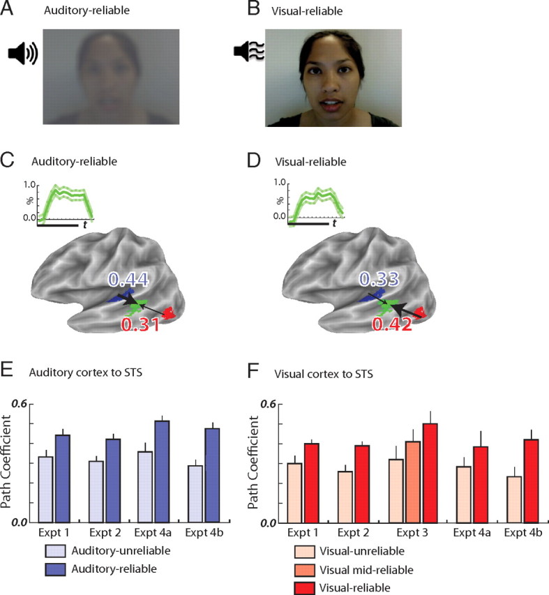
Speech stimuli and functional connectivity. A, Auditory-reliable speech: undegraded auditory speech (loudspeaker icon) with degraded visual speech (single video frame shown). B, Visual-reliable speech: undegraded visual speech with degraded auditory speech. C, STS BOLD response and functional connectivity during auditory-reliable speech in a representative subject. The inset graph shows the BOLD percentage signal change to blocks of speech (thick green line shows mean response; thin green lines show SEM; thick black bar shows 20 s duration of each block). The green region on the cortical surface model shows the location of the STS ROI. The blue number is the path coefficient between the STS ROI and the auditory cortex ROI (shown in blue); the red number is the path coefficient between the STS ROI and the visual cortex ROI (shown in red). Lateral view of the partially inflated left hemisphere, dark gray shows sulcal depths, light gray shows gyral crowns. D, STS BOLD response and functional connectivity during visual-reliable speech, same subject as in C. E, STS–auditory cortex functional connectivity in experiments 1, 2, 4A (attention to auditory modality), and 4B (attention to visual modality). Light blue bars, Path coefficients during auditory-unreliable speech. Dark blue bars, Path coefficients during auditory-reliable speech. F, STS–visual cortex functional connectivity in experiments 1–4.
Reliable (non-noisy) speech consisted of the original recordings without any degradation. Unreliable (noisy) speech was created by independently degrading the auditory and visual components of the recordings. The auditory stimulus was degraded in Matlab (MathWorks) using a noise-vocoded filter to modulate noise within the temporal envelope of the stimulus in four separate frequency bands (0–800 Hz, 800–1500 Hz, 1500–2500 Hz, and 2500–4000 Hz), and the smoothing frequency, or sampling rate of the temporal envelope of each frequency band of the noise-vocoded speech, was 300 Hz (Shannon et al., 1995). The visual stimulus was degraded by individually filtering each frame of the video in Matlab. First, the contrast of the frame was decreased by 70%, and then the frame was blurred with a Gaussian filter (the filter size depended on the stimulus condition; see below). Both of these methods for degrading speech decrease intelligibility: vocoding auditory speech stimuli decreases recognition scores (Shannon et al., 1995), and decreasing the spatial resolution of visual speech stimuli decreases word identification (Munhall et al., 2004).
General fMRI methods
At the beginning of each scanning session, two T1-weighted MP-RAGE anatomical MRI scans were collected at 3 tesla using an eight-channel head gradient coil; the anatomical scans were aligned to each other and averaged to provide maximum gray-white contrast. Then, a cortical surface model was created with FreeSurfer (Dale et al., 1999; Fischl et al., 1999) to allow visualization and region-of-interest creation with SUMA (Argall et al., 2006). T2*-weighted images for fMRI were collected using gradient-echo echo-planar imaging (TR = 2015 ms, TE = 30 ms, flip angle = 90°) with in-plane resolution of 2.75 × 2.75 mm. Thirty-three 3 mm axial slices were collected, resulting in whole-brain coverage in most subjects. Each functional scan series consisted of 154 brain volumes. The first four volumes, collected before equilibrium magnetization was reached, were discarded resulting in 150 usable volumes. Ear defender (acoustic earmuff) type pneumatic headphones were used to present auditory stimuli within the scanner, ensuring stimulus audibility even without the use of a sparse sampling paradigm. Visual stimuli were projected onto a screen using an LCD projector and viewed through a mirror attached to the head coil. Behavioral responses were collected using a fiber-optic button response pad (Current Designs). MR-compatible eye tracking (Applied Science Laboratories) was used in all fMRI experiments to ensure alertness and visual fixation.
fMRI data analysis was performed using the freely available software packages “R” (Ihaka and Gentleman, 1996) and Analysis of Functional NeuroImages software (AFNI) (Cox, 1996). Appendices A–C contain the complete list of commands used to analyze data in experiments 1 and 2 to facilitate replication of our analyses. Corrections for voxelwise multiple comparisons were performed using the false discovery rate procedure (Genovese et al., 2002) and reported as “q” values. Data were analyzed within each subject, and then group analyses were performed by combining data across subjects using a random-effects model.
Functional data were aligned to the average anatomical dataset and motion corrected for each voxel in each subject using a local Pearson correlation (Saad et al., 2009). All analysis was performed in all voxels in each subject in the context of the generalized linear model using a maximum-likelihood approach using the AFNI function 3dDeconvolve.
For block designs (localizer and experiment 1), a single regressor was created for each stimulus type by convolving the stimulus timing with a canonical gamma-variate estimate of the hemodynamic response function. For rapid event-related designs (experiments 2, 3, and 4), the amplitude of the hemodynamic response for each individual auditory-reliable and visual-reliable stimulus presentation was estimated. A separate regressor was created for each individual stimulus using the -stim_times_IM mode of 3dDeconvolve. Movement covariates and baseline drifts (as second-order polynomials, one per scan series) were modeled as regressors of no interest. All regressors were fit separately to each voxel.
For volumetric group analysis, each subject's average anatomical dataset was normalized to the N27 reference anatomical volume (Mazziotta et al., 2001) using the auto_tlrc function in AFNI.
fMRI functional localizer and regions of interest
A functional localizer scan series was used to identify regions of interest (ROIs) important for speech processing: auditory cortex, visual cortex, and STS. Each ROI was identified separately in each subject (for ROI sizes and locations, see Table 2). The ROIs were then applied to independent reliability-weighting data collected in separate scan series, preventing bias (Kriegeskorte et al., 2009). ROIs were created in both left and right hemispheres, although our analysis focused on the left hemisphere because the left hemisphere is usually dominant for language (Branch et al., 1964; Ellmore et al., 2010).
Table 2.
ROIs from fMRI localizer
| ROI | Size (mm3) | Talairach coordinates (mm) |
||
|---|---|---|---|---|
| x | y | z | ||
| Auditory | 3108 ± 969 | −45.4 ± 4.1 | −17.5 ± 3.6 | 6.1 ± 2.7 |
| Visual | 3111 ± 1068 | −42.4 ± 3.6 | −66.5 ± 4.9 | 3.1 ± 3.9 |
| STS | 3611 ± 1210 | −48.8 ± 2.9 | −46 ± 6.4 | 9.7 ± 3.8 |
Average size and location of individual auditory, visual, and STS ROIs created from functional localizers across all subjects (mean ± SD). Sample subject ROIs are shown in Figure 1, C and D.
The functional localizer scan series contained 10 blocks (five unisensory auditory and five unisensory visual in random order) of duration 20 s with 10 s of fixation baseline between each block. Each block contained ten 2 s trials, each containing one undegraded word. All ROIs were created on the cortical surface using SUMA for maximum anatomical precision. The auditory cortex ROI was defined using the contrast of auditory speech versus baseline to find active voxels within Heschl's gyrus, demarcated by the superior temporal gyrus at the lateral/inferior boundary, the first temporal sulcus at the anterior boundary, the transverse temporal sulcus at the posterior boundary, and the medial termination of Heschl's gyrus at the medial/superior boundary (Patterson and Johnsrude, 2008; Upadhyay et al., 2008). The visual cortex ROI was defined using the contrast of visual speech versus baseline to find active voxels along the inferior temporal sulcus (ITS) or its posterior continuation near areas LO and MT (Dumoulin et al., 2000) within extrastriate lateral occipital cortex, a brain region critical for processing moving and biological stimuli that includes the middle temporal visual area and the extrastriate body area (Tootell et al., 1995; Beauchamp et al., 1997, 2002, 2003; Downing et al., 2001; Pelphrey et al., 2005). The STS ROI was defined using a conjunction analysis to find all voxels that responded to both auditory and visual speech significantly greater than baseline in the anatomically defined posterior STS (q < 0.05 for each modality) (Beauchamp, 2005a; Beauchamp et al., 2008).
Structural equation modeling
To test the hypothesis that connection weights would be different for auditory-reliable and visual-reliable speech, a structural equation model was constructed and tested for each stimulus condition in each subject in each experiment. Path coefficients from the models were compared across subjects using an ANOVA.
The model consisted of the three ROIs (auditory cortex, visual cortex, and STS) in the left hemisphere with unidirectional connections between auditory cortex and STS and between visual cortex and STS (for ROIs in one subject, see Fig. 1C,D). Models were also tested consisting of bidirectional connections between the left-hemisphere ROIs and unidirectional connections between right-hemisphere ROIs. In addition, we performed a whole-brain connectivity analysis on the experiment 1 data to determine whether any other regions outside the auditory and visual cortex ROIs showed condition-dependent changes in connection strength with STS, similar to a psychophysiological interaction (Friston et al., 1997). The whole-brain connectivity analysis was first performed in each subject and then averaged across subjects using an ANOVA.
Experiment 1: fMRI block design
fMRI experimental design.
To minimize the number of stimulus conditions in experiments 1 and 2, reliable stimuli in one modality were paired with unreliable stimuli in the other modality, resulting in only two conditions: auditory-reliable (auditory-reliable + visual-unreliable) and visual-reliable (visual-reliable + auditory-unreliable). Unreliable videos were created by blurring with a 30 pixel diameter Gaussian filter. Three reliability scan series were presented to each subject. Scan series contained five blocks of auditory-reliable and five blocks of visual-reliable congruent words. Each 20 s block contained ten 2 s trials, with one different word per trial (10 words total per block). Each video ranged in length from 1.1 to 1.8 s with fixation crosshairs occupying the remainder of each 2 s trial. Each block contained a different set of randomly selected words. There were 10 s of fixation baseline between each block, for a total scan series time of 5 min.
fMRI data analysis.
As shown in Figure 1, stimulus blocks evoked a robust blood oxygenation level-dependent (BOLD) signal consisting of a typical square-wave-like response. A generalized linear model analysis was used to calculate the average amplitude of response to each stimulus type in each ROI. However, analysis of fMRI time series containing these large block onsets and offsets produces a very high correlation between ROIs that obscures differences in functional connectivity (Büchel and Friston, 1997). Therefore, for the connectivity analysis in each subject, these block onset and offset responses (defined as the best fit of the block-design regressors) were subtracted from the time series in each voxel, as were the best-fit regressors of no interest for that voxel, using the AFNI function 3dSynthesize (see Appendix A for the details of all functions used in the analysis). Because a distinct set of areas is active during baseline conditions in the so-called default-mode network (Raichle et al., 2001), our connectivity analysis only examined the 10 volumes per block collected during word presentation (150 time points for each condition, consisting of 15 blocks of each stimulus type times 10 time points per block). The residual time series for each condition was averaged across all voxels in each ROI to create two time series for each ROI (one per condition). The residual time series were used to calculate the correlation matrix and path coefficients for each condition using the AFNI functions 1ddot and 1dsem (Chen et al., 2007). Two-way ANOVAs were performed in MATLAB with condition (auditory-reliable or visual-reliable) and sensory cortex (auditory or visual) as fixed factors, subject as a random factor, and amplitude of response and path coefficient as the dependent measures.
Whole-brain connectivity: psychophysiological interactions.
The ROI analysis determined whether the connectivity between auditory cortex, visual cortex, and STS differed across conditions. To determine whether any other brain regions showed differing connectivity with the STS, we performed a whole-brain connectivity analysis similar to a psychophysiological interaction (Friston et al., 1997). The time series for each condition was created consisting of the concatenated residual time series for the auditory-reliable and visual-reliable stimulation blocks (see Appendix B for details). A generalized linear model analysis was performed on this dataset using three regressors of interest. The first regressor (physiological factor) consisted of the residual time series from the STS ROI. The second regressor (psychological factor) consisted of 150 values of +1 (corresponding to the 150 visual-reliable time points) and 150 values of −1 (corresponding to the 150 auditory-reliable time points). The third regressor (the psychophysiological factor) consisted of the first regressor multiplied by the second regressor. Voxels with a significant amount of variance accounted for by the third regressor show a different slope relating activity in the STS to activity in the target region as a function of condition. The t-statistic of the psychophysiological factor and the t-statistic of the full model from each individual subject were averaged across subjects using a voxelwise ANOVA to find all voxels that showed a significant response to a threshold of all word stimuli (q < 0.0095) and a significant difference in correlation with the STS across conditions (q < 0.05).
Experiment 2: fMRI rapid event-related design
Two reliability scan series were presented to each subject, each containing 60 auditory-reliable word trials (2 s each), 60 visual-reliable word trials (2 s each), and 30 null trials (2 s of fixation baseline) presented pseudorandomly in optimal rapid event-related order (Dale, 1999). The amplitude of the hemodynamic response was estimated for each individual word stimulus and averaged within each ROI to produce a vector of 60 auditory-reliable word amplitudes and 60 visual-reliable word amplitudes (see Appendix C for details). These amplitudes were used to calculate the correlation matrix and path coefficients for each condition in each subject using the AFNI functions 1ddot and 1dsem. The path coefficients were then entered into the group ANOVA.
Experiment 3: fMRI rapid event-related parametric design
To create a parametric design in experiment 3, the auditory unreliable words from experiments 1 and 2 were paired with visual words that were either the same word (congruent; 50% of trials) or a different word (incongruent). Subjects made a two-alternative forced choice (2-AFC) about each stimulus using a button press (congruent vs incongruent). The visual words were reliable (unblurred) or blurred with one of three Gaussian filter widths: 5 pixels, 15 pixels, or 30 pixels. Three reliability scan series were presented to each subject. Each scan series contained 30 trials of each of the four stimulus types (120 total) and 30 trials of fixation baseline in optimized order. The behavioral and fMRI data from the 5 and 15 pixel stimuli did not differ significantly, so they were collapsed for the final analysis, resulting in three levels: reliable visual (unblurred); unreliable, blurred visual (30-pixel-width blur, the same as used in experiments 1 and 2); and intermediate midblur (5- and 15-pixel-width blur). The three conditions were then analyzed as in experiment 2.
Experiment 4: attention experiment
Although the event-related designs of experiments 2 and 3 eliminated the effect of sustained attention over the course of a block, subjects could still have reallocated attention on a trial-by-trial basis. Therefore, in experiment 4, we manipulated the behavioral task to explicitly direct subjects' attention to either the auditory or visual modality during presentation of auditory-reliable and visual-reliable syllables. A rapid event-related design was used in which auditory-reliable and visual-reliable congruent syllable stimuli were randomly intermixed. Subjects performed a behavioral 2-AFC task that directed their attention to either modality.
The stimuli consisted of two instances of syllable “ja” and two instances of “ma,” one with the speaker's eyes open and one with the speaker's eyes closed. For the auditory attention task, subjects discriminated the syllables (“ja” vs “ma”). For the visual attention task, subjects discriminated the visual appearance of the speaker (eyes open vs eyes closed).
Our choice of different auditory and visual tasks was motivated by several competing desires. First, we wished subjects to maintain attention to the auditory or visual speech, to ensure a high level of activity in STS. This ruled out an orthogonal discrimination task, such as detection of brightness changes at fixation or auditory beeps. Second, we wished to maintain ethological validity by using tasks that were not too different from cognitive processes that might occur during normal speech processing. We did not wish to use tasks that were so difficult that they might drive a high level of activity, obscuring the brain activity related to speech perception. This ruled out complex semantic decision tasks. Third, we wished to make information from the opposing modality uninformative for the task. There was absolutely no information about eyes open or eyes closed in the auditory stimulus, so subjects' optimal strategy would be to ignore the auditory modality, presumably enhancing any effect of attention and reducing any effect of reliability weighting (if reliability weighting depended on voluntary attention to the auditory modality). In contrast, if we had asked subject to perform a visual “ja” from “ma” discrimination, they could have “cheated” by using auditory information. To prevent cheating, we would have had to introduce incongruent auditory–visual stimuli, which would in itself cause changes in brain activity, since the STS is very sensitive to auditory–visual congruence (van Atteveldt et al., 2010).
Each scan series contained 120 stimuli and 30 presentations of the baseline condition in a random order. Within the 120 stimuli in each scan series, there were equal numbers of auditory-reliable and visual-reliable stimuli, equal numbers of syllables corresponding to “ja” and “ma,” and equal numbers of stimuli with the speaker's eyes open and closed. Subjects performed the auditory attention task for two scan series and the visual attention task for two scan series. Four separate structural equation models were constructed, one for each condition in each attentional state.
Experiment 5: behavioral experiment
A behavioral experiment was performed to make sure that our stimuli elicited the behavioral reliability weighting observed in previous studies. Ten healthy right-handed subjects (two female, mean age 24.8) participated in the behavioral study. To prevent ceiling effects, all stimuli were degraded more than the stimuli used in the fMRI experiments. The auditory-reliable stimuli consisted of auditory syllables noise-vocoded with a smoothing frequency of 1000 Hz and visual-unreliable syllables blurred with a 50 pixel diameter Gaussian filter, and the visual-reliable stimuli consisted of auditory-unreliable syllables noise-vocoded with a smoothing frequency of 300 Hz and visual syllables blurred with a 30 pixel diameter Gaussian filter. Congruency was manipulated in experiment 5 so that half the stimuli were congruent and half were incongruent. A 2 × 2 × 2 factorial design was used, with auditory syllable (“ma” vs “na”) as the first factor, visual syllable (“ma” vs “na”) as the second factor, and reliability (auditory-reliable vs visual-reliable) as the third factor. Auditory stimuli were delivered through headphones at ∼70 dB, and visual stimuli were presented on a computer screen. Each of 10 subjects was presented with 80 stimuli (10 examples of each stimulus type) and made a 2-AFC about their perception of each stimulus (“ma” vs “na”). Responses to incongruent stimuli (e.g., auditory “ma” + visual “na”) were analyzed with a within-subjects paired t test.
Results
The STS responded to both auditory-reliable and visual-reliable audiovisual speech with a robust BOLD response (Fig. 1C,D), but there was no difference in the amplitude of the response: 0.62% for auditory-reliable versus 0.69% for visual-reliable (p = 0.18, paired t test across subjects).
Although the amplitude of the BOLD response was similar between conditions, there was a large change in STS functional connectivity: the STS was more strongly connected to a sensory cortex when that sensory modality was reliable (Fig. 1E,F). STS–auditory cortex connectivity increased from 0.33 for auditory-unreliable to 0.44 for auditory-reliable (p = 0.02, paired t test) for the blocks of words presented in experiment 1 and from 0.31 to 0.42 (p = 0.003) for the single words presented in an event-related design in experiment 2. STS–visual cortex connectivity increased from 0.30 for visual-unreliable to 0.40 for visual-reliable (p = 0.04) in experiment 1 and from 0.26 to 0.39 (p = 0.0003) in experiment 2. In experiment 3, in which a parametric design was used with single words presented at three levels of visual reliability, STS–visual cortex connectivity increased from 0.32 to 0.42 to 0.50 with increasing levels of visual reliability (ANOVA with main effect of reliability: F(1,5) = 17.9, p = 0.0005).
Whole-brain connectivity: psychophysiological interactions
Our initial analysis measured the connection strength between the STS and auditory and visual cortex ROIs created from independent functional localizers. To determine whether other brain areas also showed reliability-weighted connections, we performed a post hoc whole-brain connectivity analysis that searched for brain areas showing stimulus-dependent interactions with the STS (Fig. 2, Table 3).
Figure 2.

Whole-brain connectivity group map. A, Whole-brain connectivity analysis showing regions with differential connectivity with STS during auditory-reliable and visual-reliable words. Shown is a group map from 10 subjects with STS seed region shown in green surrounded by dashed line. Blue areas showed greater connectivity with the STS during auditory-reliable speech, and red areas showed greater connectivity during visual-reliable speech. Shown is a lateral view of the partially inflated average cortical surface, left hemisphere. B, Ventral view of the left hemisphere showing a region near the location of the fusiform face area that showed stronger connections with the STS during auditory-reliable speech. C, Dorsal view of the left hemisphere showing a region of dorsal occipital cortex, near visual area V3A, with greater STS connectivity during visual-reliable speech.
Table 3.
Whole-brain connectivity analysis
| Interaction | Brain region | Size (mm3) | Talairach coordinates |
||
|---|---|---|---|---|---|
| x | y | z | |||
| Auditory-reliable | L STG | 1427 | −63 | −33 | 8 |
| L fusiform gyrus | 210 | −43 | −67 | −16 | |
| Visual-reliable | L LOC | 202 | −43 | −79 | 2 |
| L V3a | 142 | −17 | −93 | 12 | |
Regions in the experiment 1 group dataset showing a positive interaction with STS during auditory-reliable blocks or visual-reliable blocks. The regions are illustrated in Figure 2. L, Left.
Regions with greater STS connectivity during auditory-reliable speech were concentrated in and around auditory cortex, while regions with a greater STS connectivity during visual-reliable speech were concentrated in lateral occipital cortex. These regions largely corresponded to the auditory and visual ROIs generated from the localizer. Additional regions showing differential connectivity were found in the fusiform gyrus (greater STS connectivity during auditory-reliable speech) and dorsal occipital cortex, near visual area V3A (greater STS connectivity during visual-reliable speech). Notably, neither calcarine cortex (the location of V1) nor portions of Heschl's gyrus (the location of primary auditory cortex) showed condition-dependent changes in connectivity.
BOLD amplitudes
The observed increases in functional connectivity with reliability could be driven by differential responses in sensory cortex. The amplitudes of the BOLD response in sensory cortex increased significantly for more reliable stimuli in experiments 1 and 2 [auditory cortex, experiment (Expt.) 1: 0.46% to 0.72%, p = 0.000003; Expt. 2: 0.18% to 0.36%, p = 0.0003; visual cortex: 0.38% to 0.51%, p = 0.001; 0.23% to 0.29%, p = 0.002] but not experiment 3 (0.32% to 0.34% to 0.37%, F(1,5) = 2.1, p = 0.18). If there was a simple relationship between STS connectivity and sensory cortex BOLD amplitude, we might expect to find a correlation across subjects between connectivity and amplitude. However, there was little correlation between the two in any experiment, with all p values >0.20 (auditory cortex, correlation between STS functional connectivity and BOLD amplitude, Expt. 1, r = 0.14, p = 0.70 for auditory-unreliable stimuli and r = 0.44, p = 0.20 for auditory-reliable stimuli, Expt. 2, r = −0.15, p = 0.68 and r = −0.06, p = 0.87; visual cortex, correlation between STS functional connectivity and BOLD amplitude, Expt. 1, r = 0.16, p = 0.85 for visual-unreliable stimuli and r = −0.08, p = 0.66 for visual-reliable stimuli, Expt. 2, r = −0.41, p = 0.25 and r = −0.10, p = 0.78; Expt. 3, r = −0.21, p = 0.69 for visual-unreliable, r = 0.18, p = 0.73 for visual mid-reliable, and r = −0.42, p = 0.41 for visual-reliable).
Attention experiment
Another possible cause of reliability-related changes in connection weights could be top-down factors, especially attention (Büchel and Friston, 1997; Friston and Büchel, 2000; Macaluso et al., 2000; Mozolic et al., 2008). In experiment 4, the behavioral task was manipulated to direct subjects' attention to either the auditory or visual modality during presentation of auditory-reliable or visual-reliable speech. Subjects accurately performed the instructed task (97% correct during auditory attention and 93% correct during visual attention), indicating that subjects attended to the correct modality. Despite the presence of directed attention, the changes in STS connectivity observed in experiments 1, 2, and 3 were replicated (STS–auditory cortex: 0.32 to 0.50, p = 0.00003; STS–visual cortex: 0.25 to 0.40, p = 0.002). An ANOVA demonstrated no interaction between attention and reliability (F(1,5) = 0.11, p = 0.74).
Additional analyses
Structural equation models depend on initial assumptions about connections within the network. When we modified the model to include bidirectional connections or right hemisphere regions of interest, we observed similar, but weaker, patterns of reliability weighting. For bidirectional connections, STS–auditory cortex connectivity increased from 0.55 to 0.60 (p = 0.10) in experiment 1 and from 0.45 to 0.53 (p = 0.01) in experiment 2, and STS–visual cortex connectivity increased from 0.55 to 0.59 (p = 0.13) in experiment 1, 0.45 to 0.50 (p = 0.01) in experiment 2, and 0.51 to 0.62 to 0.68 (F(1,5) = 39.1, p = 0.00002) in experiment 3. For right hemisphere regions of interest, STS–auditory cortex connectivity increased from 0.39 to 0.47 (p = 0.15) in experiment 1 and from 0.40 to 0.50 (p = 0.007) in experiment 2, and STS–visual cortex connectivity increased from 0.28 to 0.32 (p = 0.42) in experiment 1, 0.20 to 0.26 (p = 0.03) in experiment 2, and 0.45 to 0.40 to 0.53 (F(1,5) = 1.9, p = 0.21) in experiment 3.
Behavioral experiment
To replicate previous studies demonstrating that the perception of audiovisual speech is driven by the more reliable sensory modality, in experiment 5 we created incongruent stimuli whose reliability was altered using the techniques of experiments 1–4. When subjects were presented with incongruent stimuli that were reliable in one modality and unreliable in the other modality, they were more likely to classify the stimulus as the syllable presented in the reliable modality (p = 0.0001, paired t test).
Discussion
The most important result of these experiments was the surprising finding that the functional connectivity of the STS changes dramatically during perception of noisy speech, depending on the reliability of the auditory and visual modalities. The changes in connectivity were striking: the dominant modality, defined as the sensory modality with the strongest input to STS, was determined by reliability. The changes in functional connectivity were rapid, happening within 2 s during the rapid event-related experiments (experiments 2, 3, and 4) in which auditory-reliable and visual-reliable speech was randomly intermixed. Consistent results were observed across a variety of stimuli and behavioral tasks in four experiments, suggesting that the phenomenon of reliability-weighted STS connectivity is not dependent on a particular stimulus or task.
An obvious candidate to produce rapid and large changes in functional connectivity between STS and sensory cortex is the activity within sensory cortex itself. Consistent with this idea, we observed increases in the BOLD amplitude of response in sensory cortex for more reliable stimuli. This is consistent with previous fMRI studies in which auditory speech degraded using a noise-vocoded filter (as used in our study) resulted in reduced activity in auditory cortex (Scott et al., 2000; Narain et al., 2003; Giraud et al., 2004; Davis et al., 2005; Obleser et al., 2007) and low-contrast images (such as the blurred videos in our study) resulted in reduced activity in visual cortex (Callan et al., 2004; Olman et al., 2004; Park et al., 2008; Stevenson et al., 2009). While the changes in BOLD amplitude in sensory cortex in our study can be parsimoniously explained as reflecting low-level stimulus properties, we did not observe a significant correlation between STS connectivity and sensory cortex BOLD amplitude. One possible explanation is that STS neurons are driven by only a subset of neurons within sensory cortex, with a normalization that divides the strongest response in the input population by the pooled background activity (Ghose, 2009; Lee and Maunsell, 2009; Reynolds and Heeger, 2009). If we could more accurately measure the activity of this subset of neurons, perhaps using MR adaptation techniques (van Atteveldt et al., 2010), a stronger relationship between activity and connectivity might be observed.
These results can be also be interpreted in light of predictive coding models of cortical function (Kersten et al., 2004). The BOLD signal in sensory cortex is higher when a correct inference (hit) is made about auditory or visual stimuli than during misses of identical stimuli or false alarms (Hesselmann et al., 2010), suggesting that the BOLD signal in sensory cortex could be a measure of the brain's confidence about the perceptual hypothesis represented by neurons in that sensory cortex. In this model, the STS could use this confidence measure to adjust its own predictive model of the multisensory environment by adjusting its connection weights with sensory cortex.
The experimental findings are consistent with the idea that the STS is a critical brain area for auditory–visual multisensory integration (Beauchamp, 2005b). In macaque STS, a region known as STP (superior temporal polysensory) or TPO (temporo-parietal-occipital) receives projections from auditory and visual association cortex (Seltzer et al., 1996; Lewis and Van Essen, 2000) and contains single neurons that show enhanced responses to auditory and visual communication signals (Dahl et al., 2009). For brevity, we have referred to the human homolog of this region as “STS” while noting that the STS also contains other functionally and anatomically heterogeneous regions (Beauchamp, 2005b; Van Essen, 2005; Hein and Knight, 2008). During speech perception, the auditory cortex processes spectral and temporal information from the auditory vocalization, extrastriate visual cortex processes cues from lip movements, and the STS integrates the auditory and visual information (Binder et al., 1997; Price, 2000; Scott and Johnsrude, 2003; Belin et al., 2004; Hickok and Poeppel, 2007; Zatorre, 2007; Bernstein et al., 2008, 2010; Campbell, 2008; Poeppel et al., 2008). Interrupting activity in the STS reduces the McGurk effect, an illusion that depends on auditory–visual interactions (Beauchamp et al., 2010b), supporting a role for the STS in auditory–visual multisensory integration during speech (Scott and Johnsrude, 2003; Miller and D'Esposito, 2005; Campanella and Belin, 2007).
A number of behavioral studies show that the presence of information from both the auditory and visual modalities aids the perception of noisy speech (Sumby and Pollack, 1954; Hauser, 1996; Kryter, 1996; Grant and Seitz, 2000; MacDonald et al., 2000; Shahin and Miller, 2009). The perception of multisensory stimuli is reliability weighted: information from the more reliable modality is given a stronger weight (experiment 5) (Ernst and Banks, 2002; Alais and Burr, 2004). The connectivity differences we observed followed this same pattern, with more reliable sensory stimuli producing stronger connectivity between that sensory cortex and STS. If both modalities provide equivalent amounts of information, then the neural signals representing those modalities should be weighted equally. In contrast, if one modality provides poor quality information, it should receive less weighting by multisensory areas such as the STS. Therefore, it seems plausible that reliability-weighted functional connectivity between STS and sensory cortex could be the neural substrate for the reliability weighting observed behaviorally. This brain mechanism for understanding noisy speech may also be applicable to machine-learning strategies for computer-based speech recognition (Dupont and Luettin, 2000; Girin et al., 2001).
For the initial analysis, a structural equation model was selected in which auditory and visual cortex provide unidirectional projections to STS. However, there are both top-down and bottom-up connections throughout the cortical processing hierarchy (Felleman and Van Essen, 1991; Murray et al., 2002; de la Mothe et al., 2006; Winer, 2006; van Atteveldt et al., 2009). When incorporating bidirectional connections into the structural equation model, we also observed reliability weighting. Models of the right hemisphere showed weaker reliability weighting, perhaps reflecting the less important role of the right hemisphere in speech perception (Wolmetz et al., 2011).
Even without the constraints of the functional localizers (used to identify sensory cortex regions of interest), the whole-brain connectivity analysis demonstrated reliability-weighted connectivity changes between STS and auditory and extrastriate visual cortex. Interestingly, the whole-brain analysis also suggested that connectivity between core regions of auditory cortex and primary visual cortex were not reliability weighted. This may reflect the anatomical finding that STS receives strong visual input from extrastriate visual areas such as MT, but not V1, and that STS receives stronger input from auditory association areas than from core areas of auditory cortex (Seltzer and Pandya, 1994; Lewis and Van Essen, 2000; Smiley et al., 2007). A provocative finding in our dataset was the increased connection weight between STS and regions of ventral temporal cortex (near the fusiform face area) during auditory-reliable stimulation. If this region forms a node in the network for person identification (Kanwisher and Yovel, 2006; von Kriegstein et al., 2008), and auditory information is especially useful for person identification when visual information is degraded, then it would be behaviorally advantageous to increase connection weights between the fusiform face area and STS.
Behavioral studies have shown that reliability weighting occurs even if subjects are forced to attend to one modality, suggesting that reliability weighting is independent of modality-specific attention (Helbig and Ernst, 2008). Consistent with this finding, in experiment 4 we found that reliability-weighted connection changes persisted even if subjects' attention was directed to one modality or the other. Because we observed the same pattern of connectivity changes in experiments with passive word presentation (experiments 1 and 2) and with three different behavioral tasks (congruence detection in experiment 3; visual discrimination and auditory discrimination in experiment 4), attention or behavioral context is unlikely to be the sole explanation of our results.
We define “noisy” and “unreliable” stimuli operationally, as stimuli with reduced intelligibility (perceptual accuracy). Vocoded auditory speech (Davis et al., 2005; Dahan and Mead, 2010) and blurred visual speech (Thomas and Jordan, 2002; Gordon and Allen, 2009) have been used in many previous studies to reduce intelligibility. A recent study of visual–tactile integration used dynamic visual white noise, instead of blurring, to degrade the visual modality and found similar reliability-weighted changes in functional connectivity (Beauchamp et al., 2010a), suggesting that the precise method used to degrade stimuli is unlikely to explain our results.
Changes in functional connectivity have been observed in other studies of multisensory integration (Hampson et al., 2002; Horwitz and Braun, 2004; Fu et al., 2006; Patel et al., 2006; Gruber et al., 2007; Kreifelts et al., 2007; Noesselt et al., 2007; Obleser et al., 2007; Noppeney et al., 2008), with stronger weights most often observed in conditions in which multisensory stimuli result in behavioral improvements. Kreifelts et al. (2007) found that connection weights from sensory cortex to multisensory areas increased in strength during multisensory stimulation compared with unisensory stimulation. Noesselt et al. (2007) observed greater functional coupling between sensory cortex and STS when audiovisual stimuli were temporally congruent than when they were not. In our study, the sensory cortex processing the more reliable modality had a stronger connection with STS. Together with these previous fMRI studies, our results suggest that increased functional coupling could be a general mechanism for promoting multisensory integration. Under situations in which multisensory integration occurs, as codified by Stein and Meredith's laws of multisensory integration (Stein and Meredith, 1993), connection strengths between sensory cortex and multisensory areas are expected to be strong.
Appendix A: Commands for Analyzing Experiment 1 Data
The following are the commands used to analyze a single-subject dataset for experiment 1.
First, we aligned the two T1 anatomical scans (“${ec}” refers to the subject's experiment code, the code for each patient used to preserve anonymity).
3dAllineate -base 3dsag_t1_2.nii -source 3dsag_t1_1.nii -prefix ${ec}anatr1_1RegTo2 -verb -warp shift_rotate -cost mi -automask -1Dfile ${ec}anatr2toanatr1
Then, we averaged the two aligned anatomical scans into one dataset.
3dmerge -gnzmean -nscale -prefix ${ec}anatavg 3dsag_t1_2.nii ${ec}anatr1_1RegTo2+orig
We created skull-stripped anatomy to which the EPI could be aligned.
3dSkullStrip -input {$ec}anatavg+orig -prefix {$ec}anatavgSS
The skull-stripped anatomy was then normalized to the N27 reference anatomical volume.
@auto_tlrc -base TT_N27+tlrc -no_ss -input {$ec}anatavgSS+orig
adwarp -apar {$ec}anatavgSS_at+tlrc -dpar {$ec}anatavg+orig
The four fMRI scan series were concatenated to one file (1–3 refer to block design reliability runs, and 4 refers to the localizer run).
3dTcat -prefix {$ec}rall fmri_1.nii fmri_2.nii fmri_3.nii fmri_4.nii
The next steps were for motion correction and distortion correction.
3dresample -master {$ec}rall+orig -dxyz 1.0 0.938 0.938 -inset {$ec}anatavgSS+orig -prefix {$ec}anatavgSScrop
align_epi_anat.py -epi2anat -anat {$ec}anatavgSS+orig -anat_has_skull no -epi {$ec}rall+orig -epi_base mean
The aligned EPI data were smoothed using a 3 × 3 × 3 mm FWHM Gaussian kernel.
3dmerge -doall -1blur_rms 3 -prefix {$ec}Albl {$ec}rall_al+orig
A mask of the EPI dataset was created.
3dAutomask -dilate 1 -prefix {$ec}maskAlbl {$ec}Albl+orig
fMRI activation maps were created through a deconvolution analysis.
3dDeconvolve -fout -tout -full_first -polort a -concat runs.txt -cbucket {$ec}mr_bucket
-input {$ec}Albl+orig -num_stimts 10 -nfirst 0 -jobs 2
-mask {$ec}maskAlbl+orig
-stim_times 1 ARblock.txt 'BLOCK(20,1)' -stim_label 1 ARblock
-stim_times 2 VRblock.txt 'BLOCK(20,1)' -stim_label 2 VRblock
-stim_times 3 Ablock.txt 'BLOCK(20,1)' -stim_label 3 Ablock
-stim_times 4 Vblock.txt 'BLOCK(20,1)' -stim_label 4 Vblock
-stim_file 5 {$ec}rall_vr_al_motion.1D'[0]' -stim_base 5
-stim_file 6 {$ec}rall_vr_al_motion.1D'[1]' -stim_base 6
-stim_file 7 {$ec}rall_vr_al_motion.1D'[2]' -stim_base 7
-stim_file 8 {$ec}rall_vr_al_motion.1D'[3]' -stim_base 8
-stim_file 9 {$ec}rall_vr_al_motion.1D'[4]' -stim_base 9
-stim_file 10 {$ec}rall_vr_al_motion.1D'[5]' -stim_base 10
-prefix {$ec}mr
The next steps describe the structural equation modeling of the block design data. First, we used 3dSynthesize to find the best fit of the block-design regressors.
3dSynthesize -cbucket {$ec}mr_bucket+orig -matrix {$ec}mr.xmat.1D -select all -prefix {$ec}mr_all
Then, the best fits of the block-design regressors were subtracted from the aligned and smoothed EPI dataset to create a residual dataset.
3dcalc -a {$ec}Albl+orig -b {$ec}mr_all+orig -prefix {$ec}mr_noall -expr “a-b”
The trials in the residual dataset corresponding to the auditory-reliable (AR) and visual-reliable (VR) blocks were extracted into separate files.
3dTcat -prefix {$ec}AR_noall {$ec}mr_noall+orig'[300..309,315..324,375..384,405..414,435..444,450..459,465..474,480..489,495..504,570..579,615..624,645..654,690..699,705..714,735..744]'
3dTcat -prefix {$ec}VR_noall {$ec}mr_noall+orig'[330..339,345..354,360..369,390..399,420..429,510..519,525..534,540..549,555..564,585..594,600..609,630..639,660..669,675..684,720..729]'
These residual time series were used to calculate the correlation matrix for each condition. The rows (left to right) and columns (top to bottom) refer to the auditory ROI, visual ROI, and STS ROI.
3dROIstats -quiet -mask {$ec}_L_ROI+orig {$ec}AR_noall+orig > AR.1D
- 1ddot -terse AR.1D
- 1.00000 0.58155 0.58876
- 0.58155 1.00000 0.51082
- 0.58876 0.51082 1.00000
3dROIstats -quiet -mask {$ec}_L_ROI+orig {$ec}VR_noall+orig > VR.1D
- 1ddot -terse VR.1D
- 1.00000 0.58355 0.60122
- 0.58355 1.00000 0.67784
- 0.60122 0.67784 1.00000
The output from 1ddot was then entered into the afni function 1dsem, which prompted the user for the number and names of the ROIs, the correlation matrix (as shown above), and the parameters of the structural equation model. For the unidirectional model, we specified unidirectional connections from auditory and visual cortex to STS; for the bidirectional model, we specified bidirectional connections. The output of the SEM from each subject was then entered into an ANOVA in Matlab for group analysis.
Appendix B: Commands for Whole-Brain Connectivity Analysis
The following are the commands used to perform the whole-brain connectivity analysis (PPI) for experiment 1. First, the commands in Appendix A were executed, followed by these additional commands.
The auditory-reliable and visual-reliable residual time courses were concatenated together.
3dTcat -prefix {$ec}RelWt_noall {$ec}AR_noall+orig {$ec}VR_noall+orig
A generalized linear model analysis was performed on this dataset using three regressors of interest: the residual time series from the STS ROI, 150 values of +1 (150 auditory-reliable time points) and 150 values of −1 (150 visual-reliable time points), and the first regressor multiplied by the second regressor (all regressors created in Microsoft Excel and saved as text files).
3dDeconvolve -fout -tout -full_first -polort a
-input {$ec}RelWt_noall+orig -num_stimts 9 -nfirst 0 -jobs 2
-mask {$ec}maskAlbl+orig
-stim_file 1 STSnoall.txt -stim_label 1 STSnoall
-stim_file 2 condition.txt -stim_label 2 condition
-stim_file 3 PPI_noall.txt -stim_label 3 PPI_noall
-stim_file 4 {$ec}rall_vr_al_motion.1D'[0]' -stim_base 4
-stim_file 5 {$ec}rall_vr_al_motion.1D'[1]' -stim_base 5
-stim_file 6 {$ec}rall_vr_al_motion.1D'[2]' -stim_base 6
-stim_file 7 {$ec}rall_vr_al_motion.1D'[3]' -stim_base 7
-stim_file 8 {$ec}rall_vr_al_motion.1D'[4]' -stim_base 8
-stim_file 9 {$ec}rall_vr_al_motion.1D'[5]' -stim_base 9
-prefix {$ec}PPImr
The single-subject output from each subject was then entered into a group analysis with the following command:
3dANOVA2 -overwrite -type 3 -alevels 2 -blevels 10
-dset 1 1 FPPPImr+tlrc'[8]' -dset 2 1 FPPPImr+tlrc'[10]'
-dset 1 2 FRPPImr+tlrc'[8]' -dset 2 2 FRPPImr+tlrc'[10]'
-dset 1 3 FTPPImr+tlrc'[8]' -dset 2 3 FTPPImr+tlrc'[10]'
-dset 1 4 FVPPImr+tlrc'[8]' -dset 2 4 FVPPImr+tlrc'[10]'
-dset 1 5 FXPPImr+tlrc'[8]' -dset 2 5 FXPPImr+tlrc'[10]'
-dset 1 6 GFPPImr+tlrc'[8]' -dset 2 6 GFPPImr+tlrc'[10]'
-dset 1 7 GGPPImr+tlrc'[8]' -dset 2 7 GGPPImr+tlrc'[10]'
-dset 1 8 GIPPImr+tlrc'[8]' -dset 2 8 GIPPImr+tlrc'[10]'
-dset 1 9 GKPPImr+tlrc'[8]' -dset 2 9 GKPPImr+tlrc'[10]'
-dset 1 10 GMPPImr+tlrc'[8]' -dset 2 10 GMPPImr+tlrc'[10]'
-fa Stimuli -amean 1 PPI_Tstat -amean 2 AVFullFstat
-bucket 3dANOVA_PPI
Appendix C: Commands for Analyzing Experiment 2 Data
The following are the commands used to analyze a single-subject dataset for experiment 2.
First, we aligned the two T1 anatomical scans (“ec” refers to the subject's experiment code).
3dAllineate -base 3dsag_t1_2.nii -source 3dsag_t1_1.nii -prefix ${ec}anatr1_1RegTo2 -verb -warp shift_rotate -cost mi -automask -1Dfile ${ec}anatr2toanatr1
Then, we averaged the two aligned anatomical scans into one dataset.
3dmerge -gnzmean -nscale -prefix ${ec}anatavg 3dsag_t1_2.nii ${ec}anatr1_1RegTo2+orig
We created skull-stripped anatomy to which the EPI could be aligned.
3dSkullStrip -input {$ec}anatavg+orig -prefix {$ec}anatavgSS
The skull-stripped anatomy was then normalized to the N27 reference anatomical volume.
@auto_tlrc -base TT_N27+tlrc -no_ss -input {$ec}anatavgSS+orig
adwarp -apar {$ec}anatavgSS_at+tlrc -dpar {$ec}anatavg+orig
The four fMRI scan series are concatenated to one file (1–3 refer to block design reliability runs, and 4 refers to the localizer run).
3dTcat -prefix {$ec}rall fmri_1.nii fmri_2.nii fmri_3.nii fmri_4.nii
The next steps are for motion correction and distortion correction.
3dresample -master {$ec}rall+orig -dxyz 1.0 0.938 0.938 -inset {$ec}anatavgSS+orig -prefix {$ec}anatavgSScrop
align_epi_anat.py -epi2anat -anat {$ec}anatavgSS+orig -anat_has_skull no -epi {$ec}rall+orig -epi_base mean
The aligned EPI data are smoothed using a 3 × 3 × 3 mm FWHM Gaussian kernel.
3dmerge -doall -1blur_rms 3 -prefix {$ec}Albl {$ec}rall_al+orig
A mask of the EPI dataset is created.
3dAutomask -dilate 1 -prefix {$ec}maskAlbl {$ec}Albl+orig
The amplitude of the hemodynamic response was estimated for each individual word stimulus.
3dDeconvolve -fout -tout -full_first -polort a -concat runs.txt -cbucket {$ec}RERmr_bucket
-input {$ec}Albl+orig -num_stimts 10 -nfirst 0 -jobs 2
-mask {$ec}maskAlbl+orig
-stim_times_IM 1 ARevent.txt 'BLOCK(2,1)'-stim_label 1 ARevent
-stim_times_IM 2 VRevent.txt 'BLOCK(2,1)'-stim_label 2 VRevent
-stim_times_IM 3 Ablock.txt 'BLOCK(20,1)' -stim_label 3 Ablock
-stim_times_IM 4 Vblock.txt 'BLOCK(20,1)' -stim_label 4 Vblock
-stim_file 5 {$ec}rall_vr_al_motion.1D'[0]' -stim_base 5
-stim_file 6 {$ec}rall_vr_al_motion.1D'[1]' -stim_base 6
-stim_file 7 {$ec}rall_vr_al_motion.1D'[2]' -stim_base 7
-stim_file 8 {$ec}rall_vr_al_motion.1D'[3]' -stim_base 8
-stim_file 9 {$ec}rall_vr_al_motion.1D'[4]' -stim_base 9
-stim_file 10 {$ec}rall_vr_al_motion.1D'[5]' -stim_base 10
-prefix {$ec}RERmr
The trials corresponding to the auditory-reliable (AR) and visual-reliable (VR) words are extracted into separate files.
3dbucket -prefix {$ec}AR '{$ec}RERmr_bucket+orig[24-143]'
3dbucket -prefix {$ec}VR '{$ec}RERmr_bucket+orig[144-263]'
These vectors of 60 auditory-reliable word amplitudes and 60 visual-reliable word amplitudes were used to calculate the correlation matrix for each condition. The rows (left to right) and columns (top to bottom) refer to the auditory ROI, visual ROI, and STS ROI.
3dROIstats -quiet -mask {$ec}_L_ROI_v1+orig {$ec}AR+orig > AR.1D
- 1ddot -terse AR.1D
- 1.00000 0.69681 0.75244
- 0.69681 1.00000 0.70460
- 0.75244 0.70460 1.00000
3dROIstats -quiet -mask {$ec}_L_ROI_v1+orig {$ec}VR+orig > VR.1D
- 1ddot -terse VR.1D
- 1.00000 0.43685 0.57950
- 0.43685 1.00000 0.67163
- 0.57950 0.67163 1.00000
The output from 1ddot was then entered into the afni function 1dsem, which prompted the user for the number and names of the ROIs, the correlation matrix (as shown above), and the parameters of the structural equation model. For the unidirectional model, we specified unidirectional connections from auditory and visual cortex to STS; for the bidirectional model, we specified bidirectional connections. The output of the SEM from each subject was then entered into an ANOVA in Matlab for group analysis.
Footnotes
This research was supported by National Science Foundation Grant 642532 and National Institutes of Health Grants R01NS065395, TL1RR024147, and S10RR019186. We thank eight anonymous reviewers and the editors for their helpful comments and Vips Patel for assistance with MR data collection.
References
- Alais D, Burr D. The ventriloquist effect results from near-optimal bimodal integration. Curr Biol. 2004;14:257–262. doi: 10.1016/j.cub.2004.01.029. [DOI] [PubMed] [Google Scholar]
- Argall BD, Saad ZS, Beauchamp MS. Simplified intersubject averaging on the cortical surface using SUMA. Hum Brain Mapp. 2006;27:14–27. doi: 10.1002/hbm.20158. [DOI] [PMC free article] [PubMed] [Google Scholar]
- Beauchamp MS. Statistical criteria in FMRI studies of multisensory integration. Neuroinformatics. 2005a;3:93–113. doi: 10.1385/NI:3:2:093. [DOI] [PMC free article] [PubMed] [Google Scholar]
- Beauchamp MS. See me, hear me, touch me: multisensory integration in lateral occipital-temporal cortex. Curr Opin Neurobiol. 2005b;15:145–153. doi: 10.1016/j.conb.2005.03.011. [DOI] [PubMed] [Google Scholar]
- Beauchamp MS, Cox RW, DeYoe EA. Graded effects of spatial and featural attention on human area MT and associated motion processing areas. J Neurophysiol. 1997;78:516–520. doi: 10.1152/jn.1997.78.1.516. [DOI] [PubMed] [Google Scholar]
- Beauchamp MS, Lee KE, Haxby JV, Martin A. Parallel visual motion processing streams for manipulable objects and human movements. Neuron. 2002;34:149–159. doi: 10.1016/s0896-6273(02)00642-6. [DOI] [PubMed] [Google Scholar]
- Beauchamp MS, Lee KE, Haxby JV, Martin A. fMRI responses to video and point-light displays of moving humans and manipulable objects. J Cogn Neurosci. 2003;15:991–1001. doi: 10.1162/089892903770007380. [DOI] [PubMed] [Google Scholar]
- Beauchamp MS, Lee KE, Argall BD, Martin A. Integration of auditory and visual information about objects in superior temporal sulcus. Neuron. 2004;41:809–823. doi: 10.1016/s0896-6273(04)00070-4. [DOI] [PubMed] [Google Scholar]
- Beauchamp MS, Yasar NE, Frye RE, Ro T. Touch, sound and vision in human superior temporal sulcus. Neuroimage. 2008;41:1011–1020. doi: 10.1016/j.neuroimage.2008.03.015. [DOI] [PMC free article] [PubMed] [Google Scholar]
- Beauchamp MS, Pasalar S, Ro T. Neural substrates of reliability-weighted visual-tactile multisensory integration. Front Syst Neurosci. 2010a;4:25. doi: 10.3389/fnsys.2010.00025. [DOI] [PMC free article] [PubMed] [Google Scholar]
- Beauchamp MS, Nath AR, Pasalar S. fMRI-guided transcranial magnetic stimulation reveals that the superior temporal sulcus is a cortical locus of the McGurk effect. J Neurosci. 2010b;30:2414–2417. doi: 10.1523/JNEUROSCI.4865-09.2010. [DOI] [PMC free article] [PubMed] [Google Scholar]
- Belin P, Fecteau S, Bédard C. Thinking the voice: neural correlates of voice perception. Trends Cogn Sci. 2004;8:129–135. doi: 10.1016/j.tics.2004.01.008. [DOI] [PubMed] [Google Scholar]
- Bernstein LE, Lu ZL, Jiang J. Quantified acoustic-optical speech signal incongruity identifies cortical sites of audiovisual speech processing. Brain Res. 2008;1242:172–184. doi: 10.1016/j.brainres.2008.04.018. [DOI] [PMC free article] [PubMed] [Google Scholar]
- Bernstein LE, Jiang J, Pantazis D, Lu ZL, Joshi A. Visual phonetic processing localized using speech and nonspeech face gestures in video and point-light displays. Hum Brain Mapp. 2010 doi: 10.1002/hbm.21139. [DOI] [PMC free article] [PubMed] [Google Scholar]
- Binder JR, Frost JA, Hammeke TA, Cox RW, Rao SM, Prieto T. Human brain language areas identified by functional magnetic resonance imaging. J Neurosci. 1997;17:353–362. doi: 10.1523/JNEUROSCI.17-01-00353.1997. [DOI] [PMC free article] [PubMed] [Google Scholar]
- Branch C, Milner B, Rasmussen T. Intracarotid sodium amytal for the lateralization of cerebral speech dominance; observations in 123 patients. J Neurosurg. 1964;21:399–405. doi: 10.3171/jns.1964.21.5.0399. [DOI] [PubMed] [Google Scholar]
- Büchel C, Friston K. Interactions among neuronal systems assessed with functional neuroimaging. Rev Neurol (Paris) 2001;157:807–815. [PubMed] [Google Scholar]
- Büchel C, Friston KJ. Modulation of connectivity in visual pathways by attention: cortical interactions evaluated with structural equation modelling and fMRI. Cereb Cortex. 1997;7:768–778. doi: 10.1093/cercor/7.8.768. [DOI] [PubMed] [Google Scholar]
- Callan DE, Jones JA, Munhall K, Kroos C, Callan AM, Vatikiotis-Bateson E. Multisensory integration sites identified by perception of spatial wavelet filtered visual speech gesture information. J Cogn Neurosci. 2004;16:805–816. doi: 10.1162/089892904970771. [DOI] [PubMed] [Google Scholar]
- Calvert GA, Campbell R, Brammer MJ. Evidence from functional magnetic resonance imaging of crossmodal binding in the human heteromodal cortex. Curr Biol. 2000;10:649–657. doi: 10.1016/s0960-9822(00)00513-3. [DOI] [PubMed] [Google Scholar]
- Campanella S, Belin P. Integrating face and voice in person perception. Trends Cogn Sci. 2007;11:535–543. doi: 10.1016/j.tics.2007.10.001. [DOI] [PubMed] [Google Scholar]
- Campbell R. The processing of audio-visual speech: empirical and neural bases. Philos Trans R Soc Lond B Biol Sci. 2008;363:1001–1010. doi: 10.1098/rstb.2007.2155. [DOI] [PMC free article] [PubMed] [Google Scholar]
- Chen G, Glen DR, Stein JL, Meyer-Lindenberg AS, Saad ZS, Cox RW. Model validation and automated search in fMRI path analysis: a fast open-source tool for structural equation modeling. Paper presented at the Human Brain Mapping Conference; June; Chicago, IL. 2007. [Google Scholar]
- Cox RW. AFNI: software for analysis and visualization of functional magnetic resonance neuroimages. Comput Biomed Res. 1996;29:162–173. doi: 10.1006/cbmr.1996.0014. [DOI] [PubMed] [Google Scholar]
- Dahan D, Mead RL. Context-conditioned generalization in adaptation to distorted speech. J Exp Psychol Hum Percept Perform. 2010;36:704–728. doi: 10.1037/a0017449. [DOI] [PubMed] [Google Scholar]
- Dahl CD, Logothetis NK, Kayser C. Spatial organization of multisensory responses in temporal association cortex. J Neurosci. 2009;29:11924–11932. doi: 10.1523/JNEUROSCI.3437-09.2009. [DOI] [PMC free article] [PubMed] [Google Scholar]
- Dale AM. Optimal experimental design for event-related fMRI. Hum Brain Mapp. 1999;8:109–114. doi: 10.1002/(SICI)1097-0193(1999)8:2/3<109::AID-HBM7>3.0.CO;2-W. [DOI] [PMC free article] [PubMed] [Google Scholar]
- Dale AM, Fischl B, Sereno MI. Cortical surface-based analysis. I. Segmentation and surface reconstruction. Neuroimage. 1999;9:179–194. doi: 10.1006/nimg.1998.0395. [DOI] [PubMed] [Google Scholar]
- Davis MH, Johnsrude IS, Hervais-Adelman A, Taylor K, McGettigan C. Lexical information drives perceptual learning of distorted speech: evidence from the comprehension of noise-vocoded sentences. J Exp Psychol Gen. 2005;134:222–241. doi: 10.1037/0096-3445.134.2.222. [DOI] [PubMed] [Google Scholar]
- de la Mothe LA, Blumell S, Kajikawa Y, Hackett TA. Cortical connections of the auditory cortex in marmoset monkeys: core and medial belt regions. J Comp Neurol. 2006;496:27–71. doi: 10.1002/cne.20923. [DOI] [PubMed] [Google Scholar]
- de Marco G, Vrignaud P, Destrieux C, de Marco D, Testelin S, Devauchelle B, Berquin P. Principle of structural equation modeling for exploring functional interactivity within a putative network of interconnected brain areas. Magn Reson Imaging. 2009;27:1–12. doi: 10.1016/j.mri.2008.05.003. [DOI] [PubMed] [Google Scholar]
- Downing PE, Jiang Y, Shuman M, Kanwisher N. A cortical area selective for visual processing of the human body. Science. 2001;293:2470–2473. doi: 10.1126/science.1063414. [DOI] [PubMed] [Google Scholar]
- Dumoulin SO, Bittar RG, Kabani NJ, Baker CL, Jr, Le Goualher G, Bruce Pike G, Evans AC. A new anatomical landmark for reliable identification of human area V5/MT: a quantitative analysis of sulcal patterning. Cereb Cortex. 2000;10:454–463. doi: 10.1093/cercor/10.5.454. [DOI] [PubMed] [Google Scholar]
- Dupont S, Luettin J. Audio-visual speech modeling for continuous speech recognition. IEEE Trans Multimedia. 2000;2:141–151. [Google Scholar]
- Ellmore TM, Beauchamp MS, Breier JI, Slater JD, Kalamangalam GP, O'Neill TJ, Disano MA, Tandon N. Temporal lobe white matter asymmetry and language laterality in epilepsy patients. Neuroimage. 2010;49:2033–2044. doi: 10.1016/j.neuroimage.2009.10.055. [DOI] [PMC free article] [PubMed] [Google Scholar]
- Ernst MO, Banks MS. Humans integrate visual and haptic information in a statistically optimal fashion. Nature. 2002;415:429–433. doi: 10.1038/415429a. [DOI] [PubMed] [Google Scholar]
- Felleman DJ, Van Essen DC. Distributed hierarchical processing in the primate cerebral cortex. Cereb Cortex. 1991;1:1–47. doi: 10.1093/cercor/1.1.1-a. [DOI] [PubMed] [Google Scholar]
- Fischl B, Sereno MI, Dale AM. Cortical surface-based analysis. II: Inflation, flattening, and a surface-based coordinate system. Neuroimage. 1999;9:195–207. doi: 10.1006/nimg.1998.0396. [DOI] [PubMed] [Google Scholar]
- Friston KJ, Büchel C. Attentional modulation of effective connectivity from V2 to V5/MT in humans. Proc Natl Acad Sci U S A. 2000;97:7591–7596. doi: 10.1073/pnas.97.13.7591. [DOI] [PMC free article] [PubMed] [Google Scholar]
- Friston KJ, Buechel C, Fink GR, Morris J, Rolls E, Dolan RJ. Psychophysiological and modulatory interactions in neuroimaging. Neuroimage. 1997;6:218–229. doi: 10.1006/nimg.1997.0291. [DOI] [PubMed] [Google Scholar]
- Fu CHY, McIntosh AR, Kim J, Chau W, Bullmore ET, Williams SCR, Honey GD, McGuire PK. Modulation of effective connectivity by cognitive demand in phonological verbal fluency. Neuroimage. 2006;30:266–271. doi: 10.1016/j.neuroimage.2005.09.035. [DOI] [PubMed] [Google Scholar]
- Genovese CR, Lazar NA, Nichols T. Thresholding of statistical maps in functional neuroimaging using the false discovery rate. Neuroimage. 2002;15:870–878. doi: 10.1006/nimg.2001.1037. [DOI] [PubMed] [Google Scholar]
- Ghose GM. Attentional modulation of visual responses by flexible input gain. J Neurophysiol. 2009;101:2089–2106. doi: 10.1152/jn.90654.2008. [DOI] [PMC free article] [PubMed] [Google Scholar]
- Giraud AL, Kell C, Thierfelder C, Sterzer P, Russ MO, Preibisch C, Kleinschmidt A. Contributions of sensory input, auditory search and verbal comprehension to cortical activity during speech processing. Cereb Cortex. 2004;14:247–255. doi: 10.1093/cercor/bhg124. [DOI] [PubMed] [Google Scholar]
- Girin L, Schwartz J-L, Feng G. Audio-visual enhancement of speech in noise. J Acoust Soc Am. 2001;109:3007–3020. doi: 10.1121/1.1358887. [DOI] [PubMed] [Google Scholar]
- Gordon MS, Allen S. Audiovisual speech in older and younger adults: integrating a distorted visual signal with speech in noise. Exp Aging Res. 2009;35:202–219. doi: 10.1080/03610730902720398. [DOI] [PubMed] [Google Scholar]
- Grant KW, Seitz PF. The use of visible speech cues for improving auditory detection of spoken sentences. J Acoust Soc Am. 2000;108:1197–1208. doi: 10.1121/1.1288668. [DOI] [PubMed] [Google Scholar]
- Gruber O, Müller T, Falkai P. Dynamic interactions between neural systems underlying different components of verbal working memory. J Neural Transm. 2007;114:1047–1050. doi: 10.1007/s00702-007-0634-7. [DOI] [PubMed] [Google Scholar]
- Hampson M, Peterson BS, Skudlarski P, Gatenby JC, Gore JC. Detection of functional connectivity using temporal correlations in MR images. Hum Brain Mapp. 2002;15:247–262. doi: 10.1002/hbm.10022. [DOI] [PMC free article] [PubMed] [Google Scholar]
- Hauser MD. Cambridge, MA: MIT Press; 1996. The evolution of communication. [Google Scholar]
- Hein G, Knight RT. Superior temporal sulcus— it's my area: or is it? J Cogn Neurosci. 2008;20:2125–2136. doi: 10.1162/jocn.2008.20148. [DOI] [PubMed] [Google Scholar]
- Helbig HB, Ernst MO. Visual-haptic cue weighting is independent of modality-specific attention. J Vis. 2008;8:21, 21–16. doi: 10.1167/8.1.21. [DOI] [PubMed] [Google Scholar]
- Hesselmann G, Sadaghiani S, Friston KJ, Kleinschmidt A. Predictive coding or evidence accumulation? False inference and neuronal fluctuations. PLoS ONE. 2010;5:e9926. doi: 10.1371/journal.pone.0009926. [DOI] [PMC free article] [PubMed] [Google Scholar]
- Hickok G, Poeppel D. The cortical organization of speech perception. Nat Rev Neurosci. 2007;8:393–402. doi: 10.1038/nrn2113. [DOI] [PubMed] [Google Scholar]
- Horwitz B, Braun AR. Brain network interactions in auditory, visual and linguistic processing. Brain Lang. 2004;89:377–384. doi: 10.1016/S0093-934X(03)00349-3. [DOI] [PubMed] [Google Scholar]
- Horwitz B, Warner B, Fitzer J, Tagamets MA, Husain FT, Long TW. Investigating the neural basis for functional and effective connectivity. Application to fMRI. Philos Trans R Soc Lond B Biol Sci. 2005;360:1093–1108. doi: 10.1098/rstb.2005.1647. [DOI] [PMC free article] [PubMed] [Google Scholar]
- Ihaka R, Gentleman R. R: a language for data analysis and graphics. J Comput Graph Stat. 1996;5:299–314. [Google Scholar]
- Kanwisher N, Yovel G. The fusiform face area: a cortical region specialized for the perception of faces. Philos Trans R Soc Lond B Biol Sci. 2006;361:2109–2128. doi: 10.1098/rstb.2006.1934. [DOI] [PMC free article] [PubMed] [Google Scholar]
- Kersten D, Mamassian P, Yuille A. Object perception as Bayesian inference. Annu Rev Psychol. 2004;55:271–304. doi: 10.1146/annurev.psych.55.090902.142005. [DOI] [PubMed] [Google Scholar]
- Kreifelts B, Ethofer T, Grodd W, Erb M, Wildgruber D. Audiovisual integration of emotional signals in voice and face: an event-related fMRI study. Neuroimage. 2007;37:1445–1456. doi: 10.1016/j.neuroimage.2007.06.020. [DOI] [PubMed] [Google Scholar]
- Kriegeskorte N, Simmons WK, Bellgowan PS, Baker CI. Circular analysis in systems neuroscience: the dangers of double dipping. Nat Neurosci. 2009;12:535–540. doi: 10.1038/nn.2303. [DOI] [PMC free article] [PubMed] [Google Scholar]
- Kryter KD. New York: New York Academic; 1996. Handbook of hearing and the effects of noise. [Google Scholar]
- Lee J, Maunsell JH. A normalization model of attentional modulation of single unit responses. PLoS ONE. 2009;4:e4651. doi: 10.1371/journal.pone.0004651. [DOI] [PMC free article] [PubMed] [Google Scholar]
- Lewis JW, Van Essen DC. Corticocortical connections of visual, sensorimotor, and multimodal processing areas in the parietal lobe of the macaque monkey. J Comp Neurol. 2000;428:112–137. doi: 10.1002/1096-9861(20001204)428:1<112::aid-cne8>3.0.co;2-9. [DOI] [PubMed] [Google Scholar]
- Ma WJ, Zhou X, Ross LA, Foxe JJ, Parra LC. Lip-reading aids word recognition most in moderate noise: a Bayesian explanation using high-dimensional feature space. PLoS ONE. 2009;4:e4638. doi: 10.1371/journal.pone.0004638. [DOI] [PMC free article] [PubMed] [Google Scholar]
- Macaluso E, Frith C, Driver J. Selective spatial attention in vision and touch: unimodal and multimodal mechanisms revealed by PET. J Neurophysiol. 2000;83:3062–3075. doi: 10.1152/jn.2000.83.5.3062. [DOI] [PubMed] [Google Scholar]
- MacDonald J, Andersen S, Bachmann T. Hearing by eye: how much spatial degradation can be tolerated? Perception. 2000;29:1155–1168. doi: 10.1068/p3020. [DOI] [PubMed] [Google Scholar]
- Mazziotta J, Toga A, Evans A, Fox P, Lancaster J, Zilles K, Woods R, Paus T, Simpson G, Pike B, Holmes C, Collins L, Thompson P, MacDonald D, Iacoboni M, Schormann T, Amunts K, Palomero-Gallagher N, Geyer S, Parsons L, et al. A probabilistic atlas and reference system for the human brain: International Consortium for Brain Mapping (ICBM) Philos Trans R Soc Lond B Biol Sci. 2001;356:1293–1322. doi: 10.1098/rstb.2001.0915. [DOI] [PMC free article] [PubMed] [Google Scholar]
- McIntosh AR, Gonzalez-Lima F. Structural equation modeling and its application to network analysis in functional brain imaging. Hum Brain Mapp. 1994;2:2–22. [Google Scholar]
- Miller LM, D'Esposito M. Perceptual fusion and stimulus coincidence in the cross-modal integration of speech. J Neurosci. 2005;25:5884–5893. doi: 10.1523/JNEUROSCI.0896-05.2005. [DOI] [PMC free article] [PubMed] [Google Scholar]
- Mozolic JL, Joyner D, Hugenschmidt CE, Peiffer AM, Kraft RA, Maldjian JA, Laurienti PJ. Cross-modal deactivations during modality-specific selective attention. BMC Neurol. 2008;8:35. doi: 10.1186/1471-2377-8-35. [DOI] [PMC free article] [PubMed] [Google Scholar]
- Munhall KG, Kroos C, Jozan G, Vatikiotis-Bateson E. Spatial frequency requirements for audiovisual speech perception. Percept Psychophys. 2004;66:574–583. doi: 10.3758/bf03194902. [DOI] [PubMed] [Google Scholar]
- Murray SO, Kersten D, Olshausen BA, Schrater P, Woods DL. Shape perception reduces activity in human primary visual cortex. Proc Natl Acad Sci U S A. 2002;99:15164–15169. doi: 10.1073/pnas.192579399. [DOI] [PMC free article] [PubMed] [Google Scholar]
- Narain C, Scott SK, Wise RJS, Rosen S, Leff A, Iversen SD, Matthews PM. Defining a left-lateralized response specific to intelligible speech using fMRI. Cereb Cortex. 2003;13:1362–1368. doi: 10.1093/cercor/bhg083. [DOI] [PubMed] [Google Scholar]
- Noesselt T, Rieger JW, Schoenfeld MA, Kanowski M, Hinrichs H, Heinze HJ, Driver J. Audiovisual temporal correspondence modulates human multisensory superior temporal sulcus plus primary sensory cortices. J Neurosci. 2007;27:11431–11441. doi: 10.1523/JNEUROSCI.2252-07.2007. [DOI] [PMC free article] [PubMed] [Google Scholar]
- Noppeney U, Josephs O, Hocking J, Price CJ, Friston KJ. The effect of prior visual information on recognition of speech and sounds. Cereb Cortex. 2008;18:598–609. doi: 10.1093/cercor/bhm091. [DOI] [PubMed] [Google Scholar]
- Obleser J, Wise RJS, Dresner MA, Scott SK. Functional integration across brain regions improves speech perception under adverse listening conditions. J Neurosci. 2007;27:2283–2289. doi: 10.1523/JNEUROSCI.4663-06.2007. [DOI] [PMC free article] [PubMed] [Google Scholar]
- Olman CA, Ugurbil K, Schrater P, Kersten D. BOLD fMRI and psychophysical measurements of contrast response to broadband images. Vision Res. 2004;44:669–683. doi: 10.1016/j.visres.2003.10.022. [DOI] [PubMed] [Google Scholar]
- Park JC, Zhang X, Ferrera J, Hirsch J, Hood DC. Comparison of contrast-response functions from multifocal visual-evoked potentials (mfVEPs) and functional MRI responses. J Vis. 2008;8:1–12. doi: 10.1167/8.10.8. [DOI] [PMC free article] [PubMed] [Google Scholar]
- Patel RS, Bowman FD, Rilling JK. Determining hierarchical functional networks from auditory stimuli fMRI. Hum Brain Mapp. 2006;27:462–470. doi: 10.1002/hbm.20245. [DOI] [PMC free article] [PubMed] [Google Scholar]
- Patterson RD, Johnsrude IS. Functional imaging of the auditory processing applied to speech sounds. Philos Trans R Soc Lond B Biol Sci. 2008;363:1023–1035. doi: 10.1098/rstb.2007.2157. [DOI] [PMC free article] [PubMed] [Google Scholar]
- Pelphrey KA, Morris JP, Michelich CR, Allison T, McCarthy G. Functional anatomy of biological motion perception in posterior temporal cortex: an fMRI study of eye, mouth and hand movements. Cereb Cortex. 2005;15:1866–1876. doi: 10.1093/cercor/bhi064. [DOI] [PubMed] [Google Scholar]
- Poeppel D, Idsardi WJ, van Wassenhove V. Speech perception at the interface of neurobiology and linguistics. Philos Trans R Soc Lond B Biol Sci. 2008;363:1071–1086. doi: 10.1098/rstb.2007.2160. [DOI] [PMC free article] [PubMed] [Google Scholar]
- Price CJ. The anatomy of language: contributions from functional neuroimaging. J Anat. 2000;197:335–359. doi: 10.1046/j.1469-7580.2000.19730335.x. [DOI] [PMC free article] [PubMed] [Google Scholar]
- Raichle ME, MacLeod AM, Snyder AZ, Powers WJ, Gusnard DA, Shulman GL. A default mode of brain function. Proc Natl Acad Sci U S A. 2001;98:676–682. doi: 10.1073/pnas.98.2.676. [DOI] [PMC free article] [PubMed] [Google Scholar]
- Reynolds JH, Heeger DJ. The normalization model of attention. Neuron. 2009;61:168–185. doi: 10.1016/j.neuron.2009.01.002. [DOI] [PMC free article] [PubMed] [Google Scholar]
- Saad ZS, Glen DR, Chen G, Beauchamp MS, Desai R, Cox RW. A new method for improving functional-to-structural MRI alignment using local Pearson correlation. Neuroimage. 2009;44:839–848. doi: 10.1016/j.neuroimage.2008.09.037. [DOI] [PMC free article] [PubMed] [Google Scholar]
- Scott SK, Johnsrude IS. The neuroanatomical and functional organization of speech perception. Trends Neurosci. 2003;26:100–107. doi: 10.1016/S0166-2236(02)00037-1. [DOI] [PubMed] [Google Scholar]
- Scott SK, Blank CC, Rosen S, Wise RJ. Identification of a pathway for intelligible speech in the left temporal lobe. Brain. 2000;123:2400–2406. doi: 10.1093/brain/123.12.2400. [DOI] [PMC free article] [PubMed] [Google Scholar]
- Sekiyama K, Kanno I, Miura S, Sugita Y. Auditory-visual speech perception examined by fMRI and PET. Neurosci Res. 2003;47:277–287. doi: 10.1016/s0168-0102(03)00214-1. [DOI] [PubMed] [Google Scholar]
- Seltzer B, Pandya DN. Parietal, temporal, and occipital projections to cortex of the superior temporal sulcus in the rhesus monkey: a retrograde tracer study. J Comp Neurol. 1994;343:445–463. doi: 10.1002/cne.903430308. [DOI] [PubMed] [Google Scholar]
- Seltzer B, Cola MG, Gutierrez C, Massee M, Weldon C, Cusick CG. Overlapping and nonoverlapping cortical projections to cortex of the superior temporal sulcus in the rhesus monkey: double anterograde tracer studies. J Comp Neurol. 1996;370:173–190. doi: 10.1002/(SICI)1096-9861(19960624)370:2<173::AID-CNE4>3.0.CO;2-#. [DOI] [PubMed] [Google Scholar]
- Shahin AJ, Miller LM. Multisensory integration enhances phonemic restoration. J Acoust Soc Am. 2009;125:1744–1750. doi: 10.1121/1.3075576. [DOI] [PMC free article] [PubMed] [Google Scholar]
- Shannon RV, Zeng F-G, Kamath V, Wygonski J, Ekelid M. Speech recognition with primarily temporal cues. Science. 1995;270:303–304. doi: 10.1126/science.270.5234.303. [DOI] [PubMed] [Google Scholar]
- Smiley JF, Hackett TA, Ulbert I, Karmas G, Lakatos P, Javitt DC, Schroeder CE. Multisensory convergence in auditory cortex, I. Cortical connections of the caudal superior temporal plane in macaque monkeys. J Comp Neurol. 2007;502:894–923. doi: 10.1002/cne.21325. [DOI] [PubMed] [Google Scholar]
- Stein BE, Meredith MA. Cambridge, MA: MIT Press; 1993. The merging of the senses. [Google Scholar]
- Stein JL, Wiedholz LM, Bassett DS, Weinberger DR, Zink CF, Mattay VS, Meyer-Lindenberg A. A validated network of effective amygdala connectivity. Neuroimage. 2007;36:736–745. doi: 10.1016/j.neuroimage.2007.03.022. [DOI] [PubMed] [Google Scholar]
- Stevenson RA, James TW. Audiovisual integration in human superior temporal sulcus: inverse effectiveness and the neural processing of speech and object recognition. Neuroimage. 2009;44:1210–1223. doi: 10.1016/j.neuroimage.2008.09.034. [DOI] [PubMed] [Google Scholar]
- Stevenson RA, Kim S, James TW. An additive-factors design to disambiguate neuronal and areal convergence: measuring multisensory interactions between audio, visual and haptic sensory streams using fMRI. Exp Brain Res. 2009;198:183–194. doi: 10.1007/s00221-009-1783-8. [DOI] [PubMed] [Google Scholar]
- Sumby WH, Pollack I. Visual contribution to speech intelligibility in noise. J Acoust Soc Am. 1954;26:212–215. [Google Scholar]
- Thomas SM, Jordan TR. Determining the influence of Gaussian blurring on inversion effects with talking faces. Percept Psychophys. 2002;64:932–944. doi: 10.3758/bf03196797. [DOI] [PubMed] [Google Scholar]
- Tootell RB, Reppas JB, Kwong KK, Malach R, Born RT, Brady TJ, Rosen BR, Belliveau JW. Functional analysis of human MT and related visual cortical areas using magnetic resonance imaging. J Neurosci. 1995;15:3215–3230. doi: 10.1523/JNEUROSCI.15-04-03215.1995. [DOI] [PMC free article] [PubMed] [Google Scholar]
- Upadhyay J, Silver A, Knaus TA, Lindgren KA, Ducros M, Kim D-S, Tager-Flusberg H. Effective and structural connectivity in the human auditory cortex. J Neurosci. 2008;28:3341–3349. doi: 10.1523/JNEUROSCI.4434-07.2008. [DOI] [PMC free article] [PubMed] [Google Scholar]
- van Atteveldt NM, Blau VC, Blomert L, Goebel R. fMR-adaptation indicates selectivity to audiovisual content congruency in distributed clusters of human superior temporal cortex. BMC Neurosci. 2010;11:11. doi: 10.1186/1471-2202-11-11. [DOI] [PMC free article] [PubMed] [Google Scholar]
- van Atteveldt N, Roebroeck A, Goebel R. Interaction of speech and script in human auditory cortex: insights from neuro-imaging and effective connectivity. Hear Res. 2009;258:152–164. doi: 10.1016/j.heares.2009.05.007. [DOI] [PubMed] [Google Scholar]
- Van Essen DC. A population-average, landmark- and surface-based (PALS) atlas of human cerebral cortex. Neuroimage. 2005;28:635–662. doi: 10.1016/j.neuroimage.2005.06.058. [DOI] [PubMed] [Google Scholar]
- von Kriegstein K, Dogan O, Grüter M, Giraud AL, Kell CA, Grüter T, Kleinschmidt A, Kiebel SJ. Simulation of talking faces in the human brain improves auditory speech recognition. Proc Natl Acad Sci U S A. 2008;105:6747–6752. doi: 10.1073/pnas.0710826105. [DOI] [PMC free article] [PubMed] [Google Scholar]
- Werner S, Noppeney U. Superadditive responses in superior temporal sulcus predict audiovisual benefits in object categorization. Cereb Cortex. 2010;20:1829–1842. doi: 10.1093/cercor/bhp248. [DOI] [PubMed] [Google Scholar]
- Wilson M. The MRC psycholinguistic database: machine readable dictionary, version 2. Behav Res Methods Instrum Comput. 1988;20:6–11. [Google Scholar]
- Winer JA. Decoding the auditory corticofugal systems. Hear Res. 2006;212:1–8. doi: 10.1016/j.heares.2005.06.014. [DOI] [PubMed] [Google Scholar]
- Wolmetz M, Poeppel D, Rapp B. What does the right hemisphere know about phoneme categories? J Cogn Neurosci. 2011;23:552–569. doi: 10.1162/jocn.2010.21495. [DOI] [PMC free article] [PubMed] [Google Scholar]
- Wright TM, Pelphrey KA, Allison T, McKeown MJ, McCarthy G. Polysensory interactions along lateral temporal regions evoked by audiovisual speech. Cereb Cortex. 2003;13:1034–1043. doi: 10.1093/cercor/13.10.1034. [DOI] [PubMed] [Google Scholar]
- Zatorre RJ. There's more to auditory cortex than meets the ear. Hear Res. 2007;229:24–30. doi: 10.1016/j.heares.2007.01.018. [DOI] [PubMed] [Google Scholar]