

Abstract
The distributed point source method (DPSM) was recently proposed for ultrasonic field modeling and other applications. This method uses distributed point sources, placed slightly behind transducer surface, to model the ultrasound field. The acoustic strength of each point source is obtained through matrix inversion that requires the number of target points on the transducer surface to be equal to the number of point sources. In this work, DPSM was extended and further developed to overcome the limitations of the original method and provide a solid mathematical explanation of the physical principle behind the method. With the extension, the acoustic strength of the point sources was calculated as the solution to the least squares minimization problem instead of using direct matrix inversion. As numerical examples, the ultrasound fields of circular and rectangular transducers were calculated using the extended and original DPSMs which were then systematically compared with the results calculated using the theoretical solution and the exact spatial impulse response method. The numerical results showed the extended method can model ultrasonic fields accurately without the scaling step required by the original method. The extended method has potential applications in ultrasonic field modeling, tissue characterization, nondestructive testing, and ultrasound system optimization.
Keywords: distributed point source method, field modeling, nondestructive testing, noninvasive tissue characterization, spatial impulse response method
1. Introduction
Ultrasound, as one method utilized in nondestructive testing (NDT), has been widely used for characterization of materials' properties in industry, defense, and aerospace research. Nondestructive and non-invasive ultrasound is also used for quantification and characterization of biological bone tissues, such as cortical and trabecular bones, and other biomaterials [1-4]. For these purposes, the ultrasound wave propagation and diffraction in these media need to be understood. Within homogenous media, wave propagation and diffraction from a boundary or aperture are governed by the classic diffraction theory [5-7], which is based on the linear scalar wave equation. The most elegant solution to the diffraction problem is the Rayleigh-Sommerfeld (RS) formula [8]. However, the exact closed-form solution is only available for axial field points [9-11] in simple configurations because of the double integration in the RS formula.
Angular spectrum method [12-15] is a mathematically equivalent solution to the diffraction problem and has a simple physical explanation. With this method, a complicated field pattern is decomposed through a 2-D Fourier transform as a summation or integration of simple waves, propagating homogeneous waves and the ever-decaying evanescent waves. After the waves propagate for some distance, the field at the new location can be expressed as the superposition of propagating waves with adjusted phases while evanescent waves are ignored in most cases. To improve computation efficiency, the 2-D Fourier transform can be implemented through fast Fourier transform (FFT) that dramatically reduces the computation time compared to the RS formula. Because of its computational efficiency and capability of calculating the field at the transducer surface, the angular spectrum method has been studied extensively [16-28].
Another technique that can evaluate the transient field directly in time domain is called the spatial impulse response method (SIRM), derived from the Rayleigh integral and first proposed by Tupholme [29] and Stepanishen [30, 31]. With this method, the transient field is formulated as a convolution of the normal velocity function and the spatial impulse response function. In the original papers [30, 31], the closed-form solution was only given for circular pistons. The exact solution of the impulse response for rectangular planar sources was later provided by Lockwood and Willette [32] and Emeterio and Ullate [33], and solutions for other sources with different shapes have also been proposed [34-36]. Like the angular spectrum method, SIRM is capable of evaluating the field at the transducer surface.
In the past decade or so, some alternative methods [37-53] have also been proposed to speed up numerical calculations. For example, Cavanagh and Cook [37] decomposed the axial-symmetrical field produced by a circular piston to simple Gaussian beams; Berkhout and Wapenaar [40-42] developed a matrix formulation for ultrasound propagation and reflection in inhomogeneous media; Fan et al. [39, 46] calculated the axial-symmetric ultrasound field through an equivalent phased array method; Lee and Benkeser [43] divided the piston into small rectangular parts and applied the Fourier transform relationship between the far field and the aperture.
The distributed point source method (DPSM) was recently proposed by Placko and Kundu [54, 55]. It has attracted much attention in the field of non destructive evaluation [56-58]. This method uses distributed point sources, placed slightly behind the transducer surface, to model ultrasound fields. The acoustic strength of each point source is obtained through direct matrix inversion. Because discrete point sources are used, the field calculation can be formulated as highly-efficient matrix operations. This method has extensive applications in field calculation, transducer modeling and other areas [54]. However, a solid mathematical foundation of this method was not provided in previous publications although intuitive justifications for using point sources to model the transducer were suggested by Placko and Kundu [55]. In addition, the number of target points on the transducer surface must equal the number of point sources. Furthermore, the accuracy of this method was not systematically studied since only the results of axial field points were compared to theoretical results for circular transducers.
Because of its broad applications in transducer design, ultrasound system modeling, nondestructive testing and ultrasound beamforming, the DPSM was extended and further studied in this work. For the extended method, the distributed point sources were also placed slightly behind the transducer surface. However the number of target points could be larger than the number of point sources and these target points could be chosen with few restrictions. The acoustic strength of the point sources was formulated as the solution to the least squares minimization problem by using matrix formulation. This formulation laid a solid mathematical foundation for the physical principle behind the extended DPSM. As numerical examples, the ultrasound fields of circular and rectangular transducers were modeled using the original and extended DPSMs. The results were systematically compared with theoretical results and the SIRM results using exact formulation for the impulse response without any approximation [32].
2. Theory
2.1. Extension of the distributed point source method
For a rigidly-baffled planar transducer (shown in Fig. 1) in a homogeneous medium, the solution to the linear lossless wave equation can be expressed as a Rayleigh integral [17],
Fig. 1.

Geometry of the transducer and the field point. The transducer is located on the (x, y, 0) plane; ds is the surface element of the transducer; (x, y, z) is the coordinate of the field point x⃗; R is the distance between the surface element and field point; the shaded area is the rigid baffle.
| (1) |
where p(x⃗, ω0) is the pressure at field point x⃗; ω0 is the angular frequency; ρ0 is the density of the medium; v0 is the amplitude of the particle velocity that is normal to the transducer surface and distributed uniformly over the entire transducer aperture as vz = v0e−jω0t; t is the time; k = ω0/c is the wave number and c is the speed of sound in the medium; and R is the distance between the field point and surface element ds.
The aim is to use M distributed point sources (as shown in Fig. 2) in place of the transducer itself for modeling ultrasound fields. These point sources are placed on a plane that is parallel to the transducer surface and slightly behind it by a distance of rs. After sequentially labeling point sources as 1 to M, we can simplify the integration in Eq. (1) to a summation,
Fig. 2.

The positioning of distributed point sources, transducer surface and target points. The point sources are placed on a parallel plane behind the transducer surface, and the distance between them is rs; the point sources and target points are indexed by m and n, respectively; the distance between point source m and target point n is rnm.
| (2) |
where m is the index of a point source; rm is distance between point source m and field point x⃗; and pm(x⃗, ω0) is the pressure that is contributed by point source m. pm(x⃗, ω0) can be explicitly written as,
| (3) |
where Am = − jω0ρ0v0ds / 2π is defined as the acoustic strength of point source m.
By using the Euler's equation for ideal fluids [55], the z-direction particle velocity at field point x⃗ that is contributed by point source m can be derived from Eq. (3) as,
| (4) |
where zm is the distance in z direction between field point x⃗ and point source m. The total z-direction particle velocity contributed by all point sources is the summation of vzm(x⃗, ω0) and given by,
| (5) |
When N field points, sequentially labeled as 1 to N, are selected as the target points (shown in Fig. 2), the z-direction particle velocity at target point n is given by,
| (6) |
where n is the index of a target point; znm is the distance in z direction between target point n and point source m; and rnm is distance between target point n and point source m.
Arranging the strengths of point sources into a vector and separating the real parts from the imaginary parts, we have
| (7) |
where is the real part of the acoustic strength for point source m; is the imaginary part; and m = 1,⋯, M. The real and imaginary parts are separated to avoid complex vectors and complex matrixes that are not always supported for some programming environments in numerical implementations. This formulation can be easily adapted where complex systems are supported, such as in Matlab.
Following the same format, we define the z-direction particle velocities at target points as another vector,
| (8) |
where is the real part of the particle velocity as defined in Eq. (6) for target point n; is the imaginary part; and n=1,⋯,N.
Assuming As is known and using Eq. (8) and Eq. (7), we can reformulate Eq. (6) as,
| (9) |
where the matrix Mss is defined as,
| (10) |
According to Eq. (6), the elements in Eq. (10) are given by,
| (11) |
where n=1,⋯, N, and m = 1,⋯, M.
Assuming that these selected target points are located on the transducer surface plane, we can express the boundary condition at these target points for the rigidly-baffled transducer as,
| (12) |
where is the real part of the surface velocity defined by the boundary condition at target point n; is the corresponding imaginary part; and n=1,⋯,N. For the target points that are located within the transducer aperture, the real part of the velocity equals v0, and the imaginary part equals zero. For the target points that are located outside the transducer aperture, both the real and imagery parts of the velocity equal zero because the transducer is rigidly baffled.
The boundary condition at the transducer surface needs to be satisfied, which requires that Vs = vd. If the strength vector As of the point sources is known, the particle velocity vector Vs for the target points can be evaluated according to Eq. (9). By adjusting the strength vector As, we are trying to match Vs with vD by utilizing the equation as follows,
| (13) |
In Eq. (13), there are 2M variables, and 2N linear equations. When N > M, Eq. (13) is overdetermined; in most cases, there is no solution that satisfies all linear equations. Therefore, Vs would not be exactly equal to vD. To avoid this issue, we can define the square difference of these two vectors as,
| (14) |
and aim to minimize the square difference S. Minimization of S becomes the classic optimization problem in linear algebra. In the least-squares sense, the unique solution to this minimization problem is given by,
| (15) |
When N = M, Mss is a square matrix and invertible. Eq. (15) can be simplified as,
| (16) |
When N < M, Eq. (13) does not have a unique solution since the number of variables is larger than the number of linear equations.
By substituting Eq. (15) into Eq. (5), the realized z-direction particle velocity at any field point x⃗ on the transducer surface is obtained as,
| (17) |
By substituting Eq. (15) into Eq. (2), the ultrasound field at any field point x⃗ is obtained as,
| (18) |
Ideally, vz (x⃗, ω) in Eq. (17) should equal v0 everywhere within the transducer aperture, and equal zero outside of the aperture. Such an ideal condition cannot be perfectly realized because only a limited amount of point sources are used to replace the transducer that is made of a continuous surface, and Am(LS) is the optimal point strength only in the least-square sense. The unevenness of the surface velocity is the direct result of the discrete nature of these point sources. When N = M, vz(x⃗, ω) at each selected target point is indeed matched to the boundary condition according to Eq. (13) and Eq. (16) provided that Eq. (13) is not ill-conditioned. However, vz(x⃗, ω) at other points on the transducer surface are still not exactly matched. Therefore, using the distributed point sources to replace the transducer and to model ultrasound fields is a method only valid in the least-squares sense.
Solutions similar to Eq. (16) were first proposed for the original DPSM by Placko and Kundu [55]. In the original method, the target points are selected as the apexes of the spheres, which are centered at the point sources and touch the transducer surface. These distributed point sources are placed on a plane slightly behind and parallel to the transducer surface. The same number of point sources and target points is resulted. For the extended method, the target points on the transducer surface do not have to be those apexes, and the number of target points can be larger than the number of point sources.
The extended method does not limit how the point sources are distributed. For convenience, the point sources are usually distributed evenly, and each point covers an equal amount of area Δs. In this case, gap rs between the source plane and transducer plane can be set to . In effect, we are trying to use one point to replace the transducer element Δs. Therefore, the distance between the point source and the field point must be much larger than the Rayleigh distance. At such a distance, the field generated by transducer element Δs starts to resemble the field generated by a point. Because the closest distance between a point source and a field point is rs, we have,
| (19) |
where Δs/λ0 is approximately equal to the Rayleigh distance [59] for transducer element Δs and λ0 is the wavelength of the sound wave in the medium. Substituting into Eq. (19) yields,
| (20) |
From Eq. (20), the constraint on the number of point sources can be obtained as,
| (21) |
where A is the area of the transducer aperture.
For the DPSM application in this paper, rs is defined as the distance between the source plane and the transducer surface. Eq. (19)-(21) give some guidelines on how to choose the sampling pitches and total number of the point sources. Other applications of the DPSM [54, 55] defines and determines rs using different methods.
2.2. Spatial impulse response method
For SIRM, the pressure at field point x⃗ for a rigidly-baffled planar transducer (shown in Fig. 1) is given by Lockwood and Willette [32] as,
| (22) |
where H(x⃗, ω0) is the Fourier transform of the time-domain spatial impulse response h(x⃗, t) and evaluated at frequency ω0, and v0 is the amplitude of the particle velocity on the transducer surface in z direction. The exact formulation of h(x⃗, t) for circular and rectangular transducers can be found in Ref. [32].
The Fourier transform of the impulse response in Eq. (22) can be numerically implemented by FFT. The relationship between FFT and the continuous Fourier transform is given by [60],
| (23) |
where Hˆ(·) is evaluated using discrete FFT; ΔT is the sampling interval of the time-domain impulse response; Δω = 2π /N/ΔT is the sampling frequency in frequency domain after the transform; and l = ω0/Δω is the corresponding index of the frequency ω0. When l is not an integer, simple linear interpolation can be performed to obtain Hˆ (x⃗, l).
3. Numerical Examples
3.1. Simulation conditions
For field modeling, we considered two single-element transducers, one circular with a diameter of 12.7 mm and one rectangular with dimensions of 12.7 mm × 12.7 mm. The frequency ω0/2π was set to 1 MHz; the medium was water with a density ρ0 of 1000 kg/m3; speed of sound c in water was 1540 m/s; and amplitude of the surface velocity v0 was 1 m/s. The distributed point sources and the target points were evenly sampled. The sampling pitch of point sources (pS), the sampling pitch of target points (pT), the number of point sources M and the number of target points N were listed in Table 1 with corresponding row headings. For increased distinction and clarity of results presented here, when N = M the method was labeled as DPSM since direct matrix inversion was used like the original DPSM; when N > M the method was labeled as extended DPSM (eDPSM) since least squares optimization was adopted. In addition, the sampled area of the target points for eDPSM was larger than the transducer aperture, covering the entire transducer aperture and part of the rigid baffle. The radius and length of sampled areas were 1.05 times of the radius of the circular transducer and the length of rectangular transducer, respectively. The boundary condition for the points that lay outside of the transducer aperture was defined by the rigid baffle, and the surface velocity was set to zero.
Table 1. Simulation parameters and average error of the fields for the circular and rectangular transducers.
| Circular Transducer | Rectangular Transducer | ||||||||
|---|---|---|---|---|---|---|---|---|---|
| pS(mm) | 0.5 | 0.25 | 0.17 | 0.125 | 0.5 | 0.25 | 0.17 | 0.125 | |
| M | 505 | 2025 | 4389 | 8093 | 625 | 2601 | 5625 | 10201 | |
| rs(mm) | 0.25 | 0.125 | 0.085 | 0.0625 | 0.25 | 0.125 | 0.085 | 0.0625 | |
| pT(mm) | 0.5 | 0.25 | 0.17 | 0.125 | 0.5 | 0.25 | 0.17 | 0.125 | |
| N | DPSM | 505 | 2025 | 4389 | 8093 | 625 | 2601 | 5625 | 10201 |
| eDPSM | 555 | 2214 | 4823 | 8925 | 729 | 2809 | 6241 | 11449 | |
| AE(%) | DPSM | 1.37 | 0.58 | 0.46 | 0.37 | 1.53 | 0.75 | 0.65 | 0.39 |
| eDPSM | 1.19 | 0.45 | 0.36 | 0.33 | 1.84 | 0.94 | 0.73 | 0.39 | |
Abbreviations: pS = sampling pitch of point sources; pT = sampling pitch of target points; AE = average error; DPSM = distributed point source method; eDPSM = extended distributed point source method.
The DPSM, eDPSM and SIRM [32] were all implemented using C language while SIRM was used as the standard for comparison. The methods were tested under the Linux operating system on a PC (Dell Optiplex, GX620) equipped with dual processors running at 2.8 GHz and a total internal memory of 2 GB. Limited by memory size, the methods were also adapted to Matlab under the 64-bit Window operating system on a workstation (Dell Precision, T3500) equipped with 12 GB internal memory.
To calculate the absolute differences between a field and the standard field from SRIM, an error field was defined as the absolute difference between these two fields. The average error (AE) that characterizes the average deviation of the field from the standard field in an absolute sense was calculated from the error field by averaging the error at each point. AE was normalized to the maximum of the standard field and expressed as a percentage.
3.2. Field modeling for a circular transducer
The circular transducer was modeled after a physical transducer, Panametrics V303 (Olympus NDT Inc, Waltham, MA) with a diameter of 12.7 mm and a central frequency of 1.0 MHz. This transducer is often used in NDT applications. The continuous ultrasound fields for the rigidly-baffled transducer were calculated using the DPSM and eDPSM with different parameters and compared to the field calculated using SIRM. Because the analytical solution of the field, derived from the RS formula, is only available for the axial field points as per the equation [59],
| (24) |
where a is the radius of the transducer, the field calculated with SIRM was chosen as the standard for comparison when the entire field was considered together. This choice was also justified by the fact that the SIRM developed by Lockwood and Willette [32] was an exact implementation of the Rayleigh integral [17].
To facilitate comparison of the accuracy from both eDPSM and DPSM, the ultrasound fields were calculated using both methods under different sampling schemes (listed in Table 1). The results from DPSM were presented first.
3.2.1. Results from DPSM
Fig. 3 shows the continuous ultrasound fields at 1 MHz calculated using the DPSM and SIRM for the circular transducer. The dimensions for both fields were 50 mm in z direction starting from the transducer surface and 25.4 mm (double of the transducer's diameter) in radial direction sharing the same geometrical center with the transducer. The fields were normalized and log-compressed to -40 dB to show details. In panel (a), the field was calculated using DPSM with a sampling pitch of 0.5 mm for both point sources and target points; a total of 505 point sources were used. rs was set to 0.25 mm, which was smaller than λ0/4 = 0.385 mm as required by Eq. (20). In panel (b), the field was calculated using SIRM with a temporal sampling rate of 6.4 GHz. The high sampling rate was chosen to ensure the accuracy of the calculated field since lower sampling rates could introduce aliasing in the numerical implementation of the SIRM [61]. From Fig. 3, it is apparent that the normalized field calculated using DPSM has similar characteristics as the field calculated using SIRM. To further investigate the accuracy of DPSM and SIRM, the absolute field pressures at the axial points, evaluated from these two methods and the analytical solution, were plotted in Fig. 4. There were no differences between the analytical solution and the SIRM result; this reaffirmed that the field calculated using SIRM could be used as a surrogate of the analytical solution that was not readily available at other locations, such as at the non-axial field points. On the other hand, the DPSM result was significantly different from others with the maxima being significantly smaller. Similar differences were also noticed by Kundu et al. [62] where a circular transducer with a diameter of 2.54 mm at 5.0 MHz was modeled and 500 point sources were used. These two fields could be compared to each other because the linear fields were scalable and a/λ0 was almost the same for both studies.
Fig. 3.
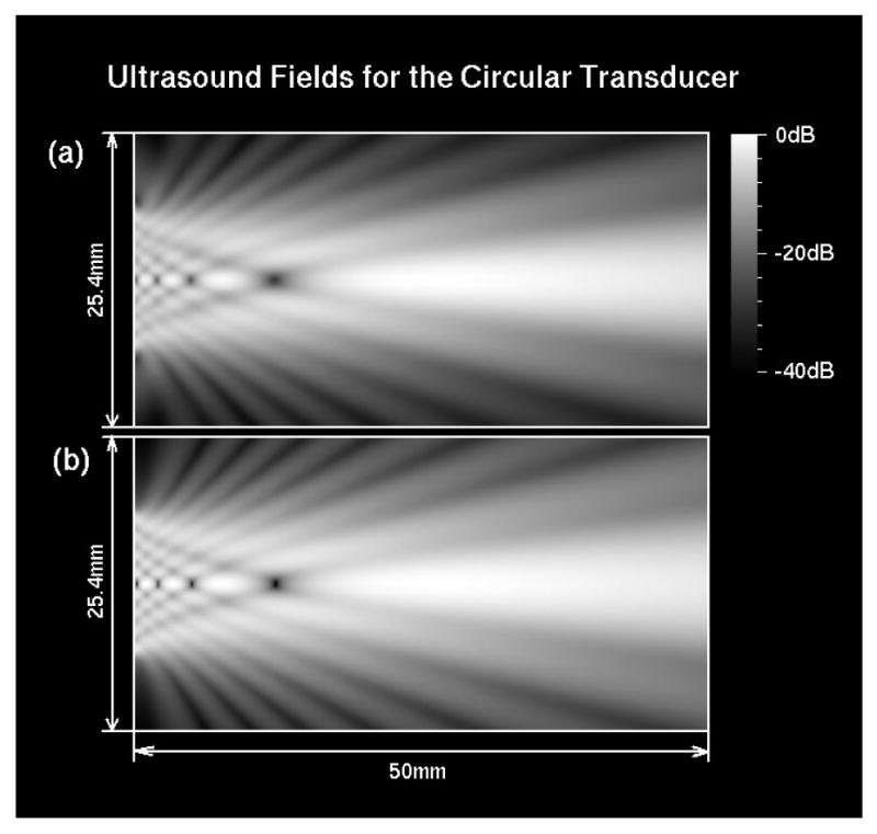
Ultrasound fields for the circular transducer at 1 MHz. (a) calculated using DPSM. pS = pT = 0.5 mm; N = M = 505. (b) calculated using SIRM. The temporal sampling rate is 6.4 GHz. The diameter of the transducer is 12.7 mm. The field is log-compressed to -40 dB.
Fig. 4.

Plots of the axial pressure calculated using DPSM, SIRM and the analytical solution. The sampling pitch of point sources and target points for DPSM is 0.5 mm and the temporal sampling rate for SRIM is 6.4 GHz.
The fields were also calculated using DPSM with other sampling pitches: 0.25 mm, 0.17 mm, and 0.125 mm. The number of point sources or target points was 2025, 4389 and 8093 respectively. All these fields have similar characteristics as the field calculated with the pitch of 0.5 mm (displayed in Fig. 3a), and are not duplicated here. However, the pressure for the axial points calculated at different sampling pitches was plotted in Fig. 5. At first glance, the results in Fig. 5 seemed to be puzzling and counterintuitive because the accuracy of the calculated pressure did not improve when finer sampling pitch and more point sources were used. The differences between the pressure calculated with DPSM and the pressure calculated with SIRM or theoretical solution, as first observed in Fig. 4, persisted even after 16 times more point sources were used. As suggested by Kundu et al. [62], the maxima of the axial pressure being significantly smaller than the theoretical prediction could be explained by the fact that the average surface velocity on the transducer surface was significantly smaller than v0 = 1 m/s, which was demanded by the boundary condition. The normal surface velocity on the transducer surface was evaluated according to Eq. (17) and displayed in Fig. 6 in linear scale as a map. The spatial sampling resolution of the velocity maps was 10 times smaller than corresponding sampling pitches of the target points. From panel (a) to (d) in Fig. 6, the sampling pitches of the velocity maps were 0.05 mm, 0.025 mm, 0.017 mm and 0.0125 mm respectively, and the average velocity on the transducer surface (ASV) was 0.845 m/s, 0.813 m/s, 0.810 m/s, and 0.808 m/s respectively. The perplexing results in Fig. 5 could be explained by the fact that average surface velocity from panel (a) to (d) in Fig. 6 was consistently smaller than 1 m/s. When more point sources were added, the distribution pattern of the surface velocity became finer while the characteristics of the pattern were kept the same. In the end, the average surface velocity was relatively constant although the density of the bright points increased dramatically from panel (a) to (d).
Fig. 5.

Plots of the axial pressure calculated using DPSM with different sampling pitches of point sources. The sampling pitches are 0.5 mm, 0.25 mm, 0.17 mm, and 0.125 mm for point sources and target points. The sampling pitches are labeled in the legend.
Fig. 6.

The surface velocity maps on the circular transducer calculated using DPSM with different sampling pitches. (a) pS = pT = 0.5 mm, (b) pS = pT= 0.25 mm, (c) pS = pT = 0.17 mm, (d) pS = pT = 0.125 mm. The velocity map is displayed in linear scale.
According to Eq. (3), the acoustic strength of the point source Am was supposed to approach – jω0ρ0v0ds / 2π when large numbers of point sources were used. Normalized by the sampling area ds, the absolute strength of the point source would be ω0ρ0v0/ 2π = 1.0×10⁹ (for clarity, the units of measure were ignored for this parameter). The average absolute strength of the point sources was 0.864×10⁹, 0.830×10⁹, 0.823×10⁹ and 0.820×10⁹ for panel (a) to (d) in Fig. 6, respectively. Like the average surface velocity, the normalized average strengths of the point sources were also consistently smaller than 1.0×10⁹.
As noticed by Kundu et al. [62], the original DPSM required an additional scaling step to accurately calculate ultrasonic fields. A scaling factor could be calculated according to the average surface velocity. For example, the average surface velocity was 0.845 m/s when the sampling pitch was 0.5 mm and the expected surface velocity was 1 m/s as demanded by the boundary condition. The scaling factor would be 1/0.845 = 1. 183. After multiplication by scaling factors, the fields at the central axis would be much closer to the theoretical results as shown in Fig. 7.
Fig. 7.

Plots of the axial pressure calculated using DPSM with scaling. The sampling pitches are 0.5 mm, 0.25 mm, 0.17 mm, and 0.125 mm for point sources and target points. The sampling pitches are labeled in the legend.
The numerical errors of entire fields, characterized by the average errors (AE) using the field calculated by the SIRM as the standard for comparison, were listed in Table 1 beginning with row heading AE. The fields calculated with DPSM were scaled by the corresponding scaling factors. The average errors were quite low and all smaller than 2%. These results reaffirmed that the original DPSM with scaling worked well.
3.2.2. Results from eDPSM
The fields calculated using the extended DPSM with four different sets of parameters (refer to Table 1) were similar to the field displayed in Fig. 3a, and were not shown to avoid duplication. The sampling pitches of the point sources were kept the same as those for DPSM; therefore, the numbers of point sources were the same too. The sampling pitches for the target points were also kept the same as those for DPSM. However, a larger area, including part of the rigid baffle, was sampled and location of the target points was different. The target points were shifted away from the source points by a distance of a quarter of the sampling pitch in both directions.
The pressure of the axial points calculated using the extended DPSM is shown in Fig. 8. Overall, eDPSM results were very close to the theoretical solutions like the DPSM results after scaling (shown in Fig. 7). The average surface velocity on the transducer surface (shown in Fig. 9), which were 1.019 m/s, 1.024 m/s, 1.021 m/s and 1.021 m/s for panel (a) to (d), respectively. These average surface velocities were very close to v0 = 1 m/s as demanded by the boundary condition. The distribution pattern of the surface velocity in Fig. 9 was quite different from that in Fig. 6. The surface velocity in Fig. 6 reached its peak, which was 1m/s, exactly at the target points, and it was smaller at all other locations. In Fig. 9, the surface velocity reached 1 m/s around the peaks, making the average surface velocity very close to 1 m/s. The average absolute strength of the point sources after normalization by the area ds was 1.019×10⁹, 1.024×10⁹, 1.021×10⁹ and 1.021×10⁹ for panel (a) to (d) in Fig. 9, respectively. Once again, the average strengths were close to 1.0×10⁹. When the entire field was considered, the accuracy of the fields calculated using eDPSM was very high (as shown in Table 1 beginning with row heading AE). The average errors for all fields were smaller than 2%, and similar to those calculated using DPSM with scaling.
Fig. 8.

Plots of the axial pressure calculated using eDPSM with different sampling pitches. The sampling pitches of are 0.5 mm, 0.25 mm, 0.17 mm, and 0.125 mm for point sources and target points. The sampling pitches are labeled in the legend.
Fig. 9.
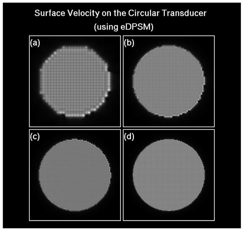
The surface velocity maps on the circular transducer calculated using eDPSM with different sampling pitches (a) pS = pT = 0.5 mm, (b) pS = pT= 0.25 mm, (c) pS = pT = 0.17 mm, (d) pS = pT = 0.125 mm. The velocity map is displayed in linear scale.
Notice that the average errors (AE) defined in this work depended on size of the area that was covered by the field. For all error calculations, the area was 25.4 mm by 50.0 mm in size as displayed in Fig. 3, and included 127,500 field points. Due to unevenness of the field, the error calculated at all field points was normalized to the maximum pressure of the standard field and expressed as a percentage. The error at each field point reflected the absolute accuracy instead of the relative accuracy for the specific field point. The AE estimated the accuracy for the entire field since the distribution of the errors was not necessarily normal.
Worth noticing was that the exact numerical implementation of DPSM in this work was slightly different from the implementation in Ref. [62] and Ref. [55], but the principles behind the them were the same. If a different implementation was adopted, the numerical results might be slightly different, but the basic trends, as observed in Fig. 5, Fig7 and Fig. 8, would be similar.
The sampling schemes for panels in Fig. 9 were by no means optimal; however, they did show that eDPSM had great potentials. The sampling scheme in Fig.9 demonstrated that the boundary condition at the transducer surface could be satisfied and the fields could be accurately calculated without the scaling step as required by the original DPSM. The extended DPSM kept the elegance and simplicity of the matrix operation from beginning to end.
3.3. Field modeling for a rectangular transducer
Fig. 10 shows the fields for the rectangular transducer calculated using DPSM and SIRM by following the same format as in Fig. 3, except that the fields in Fig. 10 lack radial symmetry due to the rectangular shape of the transducer. The field displayed in each panel of Fig. 10 was located on a plane normal to the transducer surface, parallel to two opposite edges, and through the center. The field was also calculated with different sets of parameters (listed in Table 1), using both DPSM and eDPSM. As before, all fields were quite similar and were not shown to avoid duplication. The sampling pitches for the point sources and target points were kept the same as those for the circular transducer under each sampling condition, while the numbers of point sources and target points were larger because of the transducer's rectangular shape.
Fig. 10.

Ultrasound fields for the rectangular transducer at 1 MHz. (a) calculated using DPSM. pS = pT = 0.5 mm; N = M = 625. (b) calculated using SIRM. The temporal sampling rate is 6.4 GHz. The length and width of the transducer are 12.7 mm and 12.7 mm, respectively. The fields are log-compressed to -40 dB.
The scaling step was taken for the DPSM before the average errors were calculated. The AE (listed in Table 1) showed the eDPSM and DPSM with scaling could model the ultrasonic field accurately. The AE was smaller than 2% for all fields, and became smaller when more point sources were added.
4. Conclusion
In this paper, we extended the distributed point source method. Through theoretical development, a solid mathematical foundation was established for the physical principle behind the DPSM. Based on least squares optimization, the extension maintained the simplicity and elegance of DPSM from beginning to end.
As examples, the ultrasound fields for circular and rectangular transducers were calculated using DPSM and extended DPSM with different sampling parameters. These fields were systematically compared with the standard fields calculated using SIRM. The numerical results showed that the extended DPSM provide a new way to accurately model the ultrasound field without the scaling step required by the original DPSM.
Acknowledgments
This work is kindly supported by the National Space Biomedical Research Institute through NASA Cooperative Agreement NCC 9-58, the NIH (AR52379), and US Army Medical Research.
Footnotes
Publisher's Disclaimer: This is a PDF file of an unedited manuscript that has been accepted for publication. As a service to our customers we are providing this early version of the manuscript. The manuscript will undergo copyediting, typesetting, and review of the resulting proof before it is published in its final citable form. Please note that during the production process errors may be discovered which could affect the content, and all legal disclaimers that apply to the journal pertain.
References
- 1.Lin W, Xia Y, Qin YX. Characterization of the trabecular bone structure using frequency modulated ultrasound pulse. J Acoust Soc Am. 2009;125:4071–4077. doi: 10.1121/1.3126993. [DOI] [PMC free article] [PubMed] [Google Scholar]
- 2.Xia Y, Lin W, Qin YX. Bone surface topology mapping and its role in trabecular bone quality assessment using scanning confocal ultrasound. Osteoporos Int. 2007;18:905–913. doi: 10.1007/s00198-007-0324-1. [DOI] [PubMed] [Google Scholar]
- 3.Xia Y, Lin W, Qin YX. The influence of cortical end-plate on broadband ultrasound attenuation measurements at the human calcaneus using scanning confocal ultrasound. J Acoust Soc Am. 2005;118:1801–1807. doi: 10.1121/1.1979428. [DOI] [PubMed] [Google Scholar]
- 4.Lin W, Qin YX, Rubin C. Ultrasonic wave propagation in trabecular bone predicted by the stratified model. Ann Biomed Eng. 2001;29:781–790. doi: 10.1114/1.1397787. [DOI] [PubMed] [Google Scholar]
- 5.Stratton JA. Electromagnetic theory. 1st. McGraw-Hill book company, inc.; New York, London: 1941. [Google Scholar]
- 6.Bouwkamp CJ. Diffraction theory. Rep Prog Phys. 1954;17:35–100. [Google Scholar]
- 7.Born M, Wolf E. Principles of optics. 7th. Cambridge University Press; Cambridge: 1999. [Google Scholar]
- 8.Goodman JW. Introduction to Fourier optics. 2nd. McGraw-Hill; New York: 1996. [Google Scholar]
- 9.Osterberg H, Smith LW. Closed solutions of Rayleighs diffraction integral for axial points. J Acoust Soc Am. 1961;51:1050–1054. [Google Scholar]
- 10.Marathay AS, McCalmont JF. On the usual approximation used in the Rayleigh-Sommerfeld diffraction theory. J Opt Soc Am A. 2004;21:510–516. doi: 10.1364/josaa.21.000510. [DOI] [PubMed] [Google Scholar]
- 11.Heurtley JC. Scalar Rayleigh-Sommerfeld and Kirchhoff diffraction integrals: a comparison of exact evaluations for axial points. J Opt Soc Am. 1973;63:1003–1008. [Google Scholar]
- 12.Sherman GC, Bremermann H. Generalization of the angular spectrum of plane waves and the diffraction transform. J Opt Soc Am. 1969;59:146–156. [Google Scholar]
- 13.Sherman GC. Diffracted wave fields expressible by plane-wave expansions containing only homogeneous waves. J Opt Soc Am. 1969;59:697–711. [Google Scholar]
- 14.Montgomery WD. Algebraic formulation of diffraction applied to self imaging. J Acoust Soc Am. 1968;58:1112–1124. [Google Scholar]
- 15.Labor E. Conditions for the validity of the angular spectrum of plane waves. J Opt Soc Am. 1968;58:1235–1237. [Google Scholar]
- 16.Stepanishen PR, Benjamin KC. Forward and backward projection of acoustic fields using FFT methods. J Acoust Soc Am. 1982;71:803–812. doi: 10.1121/1.390975. [DOI] [PubMed] [Google Scholar]
- 17.Williams EG, Maynard JD. Numerical evaluation of the Rayleigh integral for planar radiators using the FFT. J Acoust Soc Am. 1982;72:2020–2030. [Google Scholar]
- 18.Maynard JD, Williams EG, Lee Y. Nearfield acoustic holography: I. theory of generalized holography and the development of NAH. J Acoust Soc Am. 1985;78:1395–1413. [Google Scholar]
- 19.Veronesi WA, Maynard JD. Nearfield acoustic holography (NAH): II. holographic reconstruction algorithms and computer implementation. J Acoust Soc Am. 1987;81:1307–1322. [Google Scholar]
- 20.Williams EG. Numerical evaluation of the radiation from unbaffled, finite plates using the FFT. J Acoust Soc Am. 1983;74:343–347. [Google Scholar]
- 21.Assaad J, Rouvaen JM. Numerical evaluation of the far-field directivity pattern using the fast Fourier transform. J Acoust Soc Am. 1998;104:72–80. [Google Scholar]
- 22.Christopher PT, Parker KJ. New approaches to nonlinear diffractive field propagation. J Acoust Soc Am. 1991;90:488–499. doi: 10.1121/1.401274. [DOI] [PubMed] [Google Scholar]
- 23.Christopher PT, Parker KJ. New approaches to the linear propagation of acoustic fields. J Acoust Soc Am. 1991;90:507–521. doi: 10.1121/1.401277. [DOI] [PubMed] [Google Scholar]
- 24.Forbes M, Letcher S, Stepanishen PR. A wave vector, time-domain method of forward projecting time-dependent pressure fields. J Acoust Soc Am. 1991;90:2782–2793. [Google Scholar]
- 25.Liu DLD, Waag RC. Propagation and backpropagation for ultrasonic wavefront design. IEEE Trans Ultrason, Ferroelect,Freq Contr. 1997;44:1–13. doi: 10.1109/58.585184. [DOI] [PubMed] [Google Scholar]
- 26.Orofino DP, Pedersen PC. Efficient angular spectrum decomposition of acoustic sources-part I I : results. IEEE Trans Ultrason, Ferroelect,Freq Contr. 1993;40:250–257. doi: 10.1109/58.216838. [DOI] [PubMed] [Google Scholar]
- 27.Orofino DP, Pedersen PC. Efficient angular spectrum decomposition of acoustic sources-part I: theory. IEEE Trans Ultrason, Ferroelect,Freq Contr. 1993;40:238–249. doi: 10.1109/58.216837. [DOI] [PubMed] [Google Scholar]
- 28.Wu P, Kazys R, Stepinski T. Analysis of the numerically implemented angular spectrum approach based on the evaluation of two-dimensional acoustic fields. part II. characteristics as a function of angular range. J Acoust Soc Am. 1996;99:1349–1359. [Google Scholar]
- 29.Tupholme GE. Generation of acoustic pulses by baffled plane pistons. Mathematika. 1969;16:209–224. [Google Scholar]
- 30.Stepanishen PR. The time-dependent force and radiation impedance on a piston in a rigid infinite planar baffle. J Acoust Soc Am. 1971;49:841–849. [Google Scholar]
- 31.Stepanishen PR. Transient radiation from pistons in an infinite planar baffle. J Acoust Soc Am. 1971;49:1629–1638. [Google Scholar]
- 32.Lockwood JC, Willette JG. High-speed method for computing the exact solution for the pressure variations in the nearfield of a baffled piston. J Acoust Soc Am. 1973;53:735–741. [Google Scholar]
- 33.Emeterio JLS, Ullate LG. Diffraction impulse response of rectangular transducers. J Acoust Soc Am. 1992;92:651–662. [Google Scholar]
- 34.Harris GR. Transient field of a baffled planar piston having an arbitrary vibration amplitude distribution. J Acoust Soc Am. 1981;70:186–204. [Google Scholar]
- 35.Jensen JA. Ultrasound fields from triangular apertures. J Acoust Soc Am. 1996;100:2049–2056. [Google Scholar]
- 36.Jensen JA. A new calculation procedure for spatial impulse responses in ultrasound. J Acoust Soc Am. 1999;105:3266–3274. [Google Scholar]
- 37.Cavanagh E, Cook BD. Gaussian-Laguerre description of ultrasonic fields-numerical example circular piston. J Acoust Soc Am. 1980;67:1136–1140. [Google Scholar]
- 38.Wen JJ, Breazeale MA. A diffraction beam field expressed as the superposition of Gaussian beams. J Acoust Soc Am. 1988;83:1752–1756. [Google Scholar]
- 39.Fan X, Moros EG, Straube WL. A concentric-ring equivalent phased array method to model fields of large axisymmetric ultrasound transducers. IEEE Trans Ultrason, Ferroelect,Freq Contr. 1990;46:830–841. doi: 10.1109/58.775647. [DOI] [PubMed] [Google Scholar]
- 40.Berkhout AJ. A unified approach to acoustical reflection imaging. I: the forward model. J Acoust Soc Am. 1993;93:2005–2016. [Google Scholar]
- 41.Berkhout AJ, Wapenaar CPA. A unified approach to acoustical reflection imaging. II: the inverse problem. J Acoust Soc Am. 1993;93:2017–2023. [Google Scholar]
- 42.Wapenaar CPA, Berkhout AJ. A unified approach to acoustical reflection imaging. III: extension to the elastic situation. J Acoust Soc Am. 1993;93:2024–2034. [Google Scholar]
- 43.Lee C, Benkeser PJ. A computationally efficient method for the calculation of the transient field of acoustic radiators. J Acoust Soc Am. 1994;96:545–551. [Google Scholar]
- 44.Sahin A, Baker AC. Ultrasonic pressure fields due to rectangular apertures. J Acoust Soc Am. 1994;96:552–556. [Google Scholar]
- 45.Zhou D, Peirlinckx L, Lumori MLD, Biesen LV. Parametric modeling and estimation of ultrasonic fields using a system identification technique. J Acoust Soc Am. 1996;99:1438–1445. [Google Scholar]
- 46.Fan X, Moros EG, Straube WL. Acoustic field prediction for a single planar continuous-wave source using an equivalent phased array method. J Acoust Soc Am. 1997;102:2734–2741. doi: 10.1121/1.420327. [DOI] [PubMed] [Google Scholar]
- 47.Cahill MD, Baker AC. Numerical simulation of the acoustic field of a phased-array medical ultrasound scanner. J Acoust Soc Am. 1998;104:1274–1283. [Google Scholar]
- 48.Gridin D. A fast method for simulating the propagation of pulses radiated by a rectangular normal transducer into an elastic half-space. J Acoust Soc Am. 1998;104:3199–3211. [Google Scholar]
- 49.Stepanishen PR. Acoustic bullets/transient Bessel beams: near to far field transition via an impulse response approach. J Acoust Soc Am. 1998;103:1742–1751. [Google Scholar]
- 50.Mast TD, Hinkelman LM, Metlay LA, Orr MJ, Waag RC. Simulation of ultrasonic pulse propagation, distortion, and attenuation in the human chest wall. J Acoust Soc Am. 1999;106:3665–3677. doi: 10.1121/1.428209. [DOI] [PubMed] [Google Scholar]
- 51.Fan X, Moros EG, Straube WL. Ultrasound field estimation method using a secondary source-array numerically constructed from a limited number of pressure measurements. J Acoust Soc Am. 2000;107:3259–3265. doi: 10.1121/1.429398. [DOI] [PubMed] [Google Scholar]
- 52.Ding D, Zhang Y. Notes on the Gaussian beam expansion. J Acoust Soc Am. 2004;116:1401–1405. [Google Scholar]
- 53.McGough RJ. Rapid calculations of time-harmonic nearfield pressures produced by rectangular pistons. J Acoust Soc Am. 2004;115:1934–1941. doi: 10.1121/1.1694991. [DOI] [PMC free article] [PubMed] [Google Scholar]
- 54.Placko D, Kundu T. DPSM for modeling engineering problems. Wiley-Interscience; Hoboken, NJ: 2007. [Google Scholar]
- 55.Placko D, Kundu T. Modeling of ultrasonic field by distributed point source method. In: Kundu T, editor. Ultrasonic nondestructive evaluation : engineering and biological material characterization. CRC Press; Boca Raton, Fla: 2004. pp. 143–202. [Google Scholar]
- 56.Yanagita T, Kundu T, Placko D. Ultrasonic field modeling by distributed point source method for different transducer boundary conditions. J Acoust Soc Am. 2009;126:2331–2339. doi: 10.1121/1.3203307. [DOI] [PubMed] [Google Scholar]
- 57.Bhise P, Mukherjee A, Sharma S, Ram R. Distributed point source model for wave propagation through multi-phase systems. In: Dattaguru B, Gopalakrishnan S, Aatre VK, editors. IUTAM Symposium on Multi-Functional Material Structures and Systems. Springer; Netherlands: 2010. pp. 317–324. [Google Scholar]
- 58.Eskandarzade M, Kundu T, Liebeaux N, Placko D, Mobadersani F. Numerical simulation of electromagnetic acoustic transducers using distributed point source method. Ultrasonics. 2010;50:583–591. doi: 10.1016/j.ultras.2009.12.003. [DOI] [PubMed] [Google Scholar]
- 59.Cobbold RSC. Foundations of biomedical ultrasound. Oxford University Press; Oxford; New York: 2007. [Google Scholar]
- 60.Chu ECh. Discrete and continuous fourier transforms : analysis, applications and fast algorithms. CRC Press; Boca Raton, Fla.: 2008. [Google Scholar]
- 61.Crombie P, Bascom PAJ, Cobbold RSC. Calculating the pulsed response of linear arrays: accuracy versus computational efficiency. IEEE Trans Ultrason, Ferroelect,Freq Contr. 1997;44:997–1009. [Google Scholar]
- 62.Kundu T, Placko D, Kabiri Rahani E, Yanagita T, Minh Dao C. Ultrasonic field modelling: a comparision between analytical, semi-analystical and numerical techniques. IEEE Trans Ultrason, Ferroelect,Freq Contr. 2010;57:2795–2807. doi: 10.1109/TUFFC.2010.1753. [DOI] [PubMed] [Google Scholar]