Determining which mechanisms lead to activation in the motor cortex: a modeling study of transcranial magnetic stimulation using realistic stimulus waveforms and sulcal geometry

Abstract

Objective

To determine which mechanisms lead to activation of neurons in the motor cortex during transcranial magnetic stimulation (TMS) with different current directions and pulse waveforms.

Methods

The total electric field induced in a simplified model of a cortical sulcus by a figure-eight coil was calculated using the finite element method (FEM). This electric field was then used as the input to determine the response of compartmental models of several types of neurons.

Results

The modeled neurons were stimulated at different sites: fiber bends for pyramidal tract neurons, axonal terminations for cortical interneurons and axon collaterals, and a combination of both for pyramidal association fibers. All neurons were more easily stimulated by a PA directed electric field, except association fibers. Additionally, the second phase of a biphasic pulse was found to be more efficient than the first phase of either monophasic or biphasic pulses.

Conclusion

The stimulation threshold for different types of neurons depends on the pulse waveform and current direction. The reported results might account for the range of responses obtained in TMS of the motor cortex when using different stimulation parameters.

Significance

Modeling studies combining electric field calculations and neuronal models may lead to a deeper understanding of the effect of the TMS-induced electric field on cortical tissue, and may be used to evaluate improvements in TMS coil and waveform design.

1. Introduction

The question of which cells are excited during transcranial magnetic stimulation (TMS) of the cerebral cortex, and by which physical mechanisms, has been debated since the early days of this technique. Modeling studies made a significant contribution to our understanding of peripheral nerve magnetic stimulation but have had a more limited impact in TMS. In peripheral nerve stimulation, it has been shown theoretically and experimentally that changes in the membrane potential of long straight axons are driven primarily by the gradient of the component of the electric field along the axon, and that stimulation occurs where this component is decreasing most rapidly along the direction of the nerve (Roth and Basser, 1990; Nilsson et al., 1992; Maccabee et al., 1993). This simple description does not apply if the nerve bends sharply (Maccabee et al., 1993) or if it enters a bony foramen (Maccabee et al., 1991). In contrast, a variety of mechanisms may be involved in cortical stimulation since numerous axonal bends and terminations provide additional sites where neurons can be depolarized by a strong electric field, even in the absence of a significant electric field gradient (Amassian et al., 1992; Nagarajan et al., 1993; Roth, 1994). Furthermore, cortical neurons have a wide range of orientations relative to the applied electric field, due both to different orientations within the cortex and to cortical folding. Thus, it is conceivable that a strong tangential electric field may stimulate horizontal neurons in the crown of a gyrus (Day et al., 1989) or pyramidal neurons in the walls of the sulcus (Fox et al., 2004). Also, heterogeneity and anisotropy of the electrical conductivity of brain tissue has a significant impact on the spatial distribution of the induced electric field (e.g. De Lucia et al., 2007; Miranda et al., 2003; Miranda et al., 2007) and may therefore affect the site of stimulation. These factors increase the level of complexity involved in modeling cortical stimulation, making it more difficult to predict which neurons are stimulated during TMS than during magnetic stimulation of the peripheral nervous system.

In a recent paper (Silva et al., 2008) we used a Finite Element Method (FEM) model of a simplified cortical sulcus to calculate the amplitude of the electric field and its directional derivative parallel and perpendicular to the cortical surface. The results, which took into account cortical geometry and the orientation of the neurons within the folded cortical sheet, suggested that stimulation may take place preferentially at 1) terminations of medium caliber (5-10 μm) horizontal fibers located throughout the crown of the gyrus and aligned with the induced electric field, 2) terminations of medium caliber intracortical vertical axons, vertical pyramidal axon collaterals and terminations of pyramidal afferents, located in the lip of the gyrus and a few millimeters away from the lip, along the depth of the sulcus, 3) bends of pyramidal fibers with diameters d₀ ≥ 10 μm, in white matter just below the lip of the gyrus, and 4) bends of Betz cells along the entire surface of the vertical wall of the sulcus, with an expected maximum depth of stimulation of at least 1.5 cm below the cortical envelope. In all cases, the degree of membrane depolarization was determined by the intensity of the electric field along the axon. The effect of fiber diameter on the degree of depolarization due to a stimulus of fixed intensity was taken into account via the space constant, λ. On the other hand, the finite duration of the stimulus could only be taken into consideration in a crude manner in this steady-state analysis. It was not possible to take stimulus waveform and current direction into account, yet these two parameters greatly influence the effect of TMS.

Several studies report the outcome of TMS as a function of stimulus waveform – either monophasic or biphasic – and as a function of the direction of the current induced in the tissue – posterior-anterior (PA) or anterior-posterior (AP) for monophasic pulses, and PA-AP or AP-PA for biphasic pulses. The results found in the literature are, to a great extent, consistent. In brief, monophasic PA stimulation of the motor cortex recruits, at threshold, a wave which, because of its latency, is believed to be due to the transynaptic activation of pyramidal tract neurons (PTN) (Terao and Ugawa, 2002; Patton and Amassian, 1954). This is termed an I₁ (indirect) wave and is followed, at higher stimulus intensities, by other indirect waves (I₂ and I₃) at regular intervals of approximately 1.5 ms. At very high stimulus intensities (180-200% of the active motor threshold, AMT) a short latency wave is recruited (Di Lazzaro et al., 1998), which is termed a D-wave, since it is thought to be due to direct activation of corticospinal neurons. The latency of the TMS-recruited D-wave is similar to the latency of the wave recruited with anodal transcranial electric stimulation (aTES) (Patton and Amassian, 1954; Di Lazzaro et al., 2001b). The output of monophasic AP stimulation is generally either a late I-wave (I₃) or a D-wave (Di Lazzaro et al., 2001a). The outcome of biphasic PA-AP stimulation at threshold is usually an I₁-wave. At higher stimulus intensities, this pulse recruits I₃ and D-waves, in a pattern similar to a monophasic AP stimulus, but with somewhat longer latencies (Di Lazzaro et al., 2001a). As for biphasic AP-PA stimuli, they are reported to have a pattern of recruitments similar to monophasic PA stimuli, although at higher stimulus intensities the latencies of the waves are different from the latencies of the waves recruited by monophasic stimulus: for some patients, these latencies are longer, while for others they are shorter (Di Lazzaro et al., 2001a).

In this paper we investigate the dynamics of neuronal responses to TMS by simulating actual neurons and neuronal trajectories embedded in a simplified FEM model of a cortical fold. We model various types of neurons present in the motor cortex and determine their individual stimulation thresholds for different TMS waveforms. The time course of the membrane potential is calculated by solving the cable equation numerically for neurons immersed in a TMS-induced electric field. The spatial distribution of the electric field is calculated as described in (Silva et al., 2008) and its time course is obtained from simulated outputs of the Magstim monophasic and biphasic stimulators (Magstim 200 and Magstim Rapid, respectively). This work aims to elucidate which mechanism is likely to stimulate each neuron type, for a given pulse waveform and current direction, and to understand which neuronal populations are recruited at threshold by each of the four stimuli modeled. Additionally, the results are expected to improve upon our previous predictions (Silva et al., 2008) of the actual location and extent of stimulation in the motor cortex.

2. Methods

The variation of a neuron's transmembrane potential due to the electric field induced during TMS can be obtained by solving the cable equation (Roth and Basser, 1990; Basser and Roth, 1991; Nagarajan et al., 1993). Finding this solution requires knowledge about the electrical properties of the neuron's membrane, the temporal variation of the induced electric field and the spatial variation along the neuron of the component of the electric field, E_s, that is parallel to the neuron's local orientation. E_s is the component of the total electric field which effectively contributes to neuronal stimulation.

2.1. Computation of the electric field

In the first part of this work we calculated the electric field along lines describing the positions, lengths and paths taken in the cortex by several neurons, as described in the literature (c.f., Section 2.2). These neuronal trajectories were added to a simplified model of the motor cortex, shown in Figure 1, which has been described in detail in a previous work (Silva et al., 2008) and is similar to motor cortex models used in other modeling studies (Manola et al, 2005; Manola et al, 2007). The model includes a figure-eight planar coil placed 3 cm above the cortical surface and parallel to it. The coil parameters model the Magstim Double 70 mm coil (Thielscher and Kammer, 2002; Thielscher and Kammer, 2004; Miranda et al., 2007); the coil was placed so as to induce an electric field perpendicular to the central sulcus, located under the coil's center. PA and AP stimulation were modeled simply by changing the direction (sign) of the current in the coil.

Figure 1.

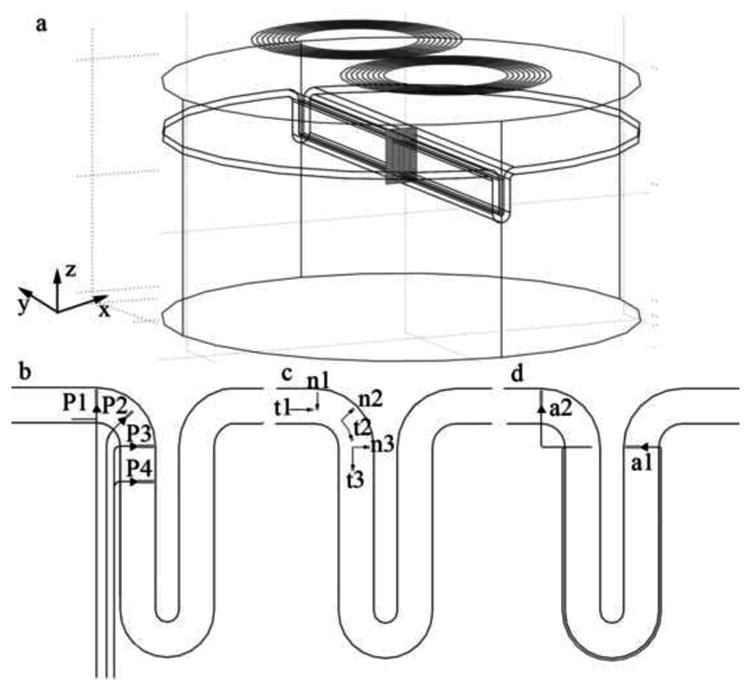
Finite Element Method (FEM) model of the motor cortex and trajectories of the 12 neurons modeled. The FEM model includes a figure-eight coil located 3 cm above the cortical surface. The plane containing the modeled neurons is shown in (a) by the gray rectangle and is located below the center of the figure-eight coil (plane y = 0). The trajectories shown in (b), (c), and (d) represent four pyramidal tract neurons (P1-P4), six cortical interneurons (t1-t3, n1-n3), and two association fibers (a1-a2), respectively. Neuron P1 comprises an axon collateral which can be located either in layer VI of the GM, as shown in the figure, or in the WM depending on the diameter of the main axon. The position of the cell bodies is represented by triangles (pyramidal cells) and circles (cortical interneurons). The dendrite is represented by a thick grey line. The motor cortex is located on the left half of the sulcus, while the somatosensory cortex is on the right half.

The total electric field, E⃗ = −∂A⃗/∂t − ∇⃗ϕ, induced in the motor cortex model was calculated using the FEM method, as implemented by the commercially available software Comsol 3.3a (www.comsol.com). This field is the sum of two terms: the first one, −∂A⃗/∂t, is the field induced by the coil itself and the second one, −(∇⃗ϕ, results from charge accumulation at the interfaces between the gray and the white matter (GM-WM) and between the cerebrospinal fluid and the gray matter (CSF-GM). In the homogeneous model, the second term is zero and the electric field is independent of the electrical conductivity. The effective electric field, E_s, along each neural trajectory was then exported from Comsol and fitted using LabFit (http://www.angelfire.com/rnb/labfit/index.htm), ZunZun.com (www.zunzun.com), or Microsoft EXCEL™.

The time variation of the total electric field, which is given by the current's time derivative, is another important parameter in neuronal stimulation (Roth and Basser, 1990; Basser and Roth, 1991). In Comsol, the current in the coil varies sinusoidally in time with a frequency, f, and a maximum intensity, I₀. However, this simplification inaccurately represents the current output of magnetic stimulators (Kammer et al., 2001). In order to take this into account we exported from Comsol the spatial distribution of E_s along the neuron at the instant of time when it was a maximum. This E_s distribution was then normalized by dividing it by the maximum value of the current's time derivative in Comsol, 2 π f I₀. Finally the normalized values of E_s along the neuron were multiplied by waveforms whose amplitudes and time courses are representative of the output of two commercially available stimulators: the Magstim 200 stimulator and the Magstim Rapid stimulator. This way we simulated the real time course of the induced electric field.

The waveforms used for both stimulators are shown in Figure 2. The Magstim 200 stimulator generates a monophasic current waveform with an approximate duration of 946 μs. The current's time derivative waveform has two peaks with opposite signs, the amplitude of the second peak being only about 0.25 of the amplitude of the first. The Magstim Rapid stimulator creates a biphasic current waveform with duration of 284 μs. The current's time derivative waveform has three peaks. The amplitude of the second peak is 0.9 of the amplitude of the first one, with an opposite sign and twice the duration of the first peak. The third peak has the same sign as the first one, about 0.8 of its amplitude and approximately the same duration. Throughout the remainder of this work, when mentioning a monophasic or biphasic waveform we will actually be referring to the current's time derivative waveforms (shown in Figure 2b), because the induced electric field is proportional to it and not to the current itself (Roth and Basser, 1990).

Figure 2.

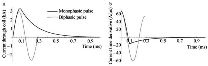
Coil current waveforms (a) and their time derivatives (b) for the monophasic and biphasic pulses modeled in this work. The terms monophasic and biphasic refer to the current waveform. The current time derivative is biphasic, for the monophasic current pulse, and triphasic, for the biphasic current pulse. The waveforms shown correspond to a charging voltage of 1107 V and a coil inductance of 16.35 μH, which yields a maximum value of 67 A/μs for the current time derivative.

All the stimulation thresholds in this work will be given in terms of the maximum value of the current's time derivative and also as the percentage of the maximum stimulator output (MSO). For the Magstim 200 stimulator, connected to the coil modelled in this work, dI/dt_Max = 171 A/μs at 100 % MSO (Kammer et al., 2001). The Magstim Rapid stimulator can be programmed to go up to dI/dt_Max=122 A/μs (Kammer et al., 2001) but at this value the stimulator's frontal panel indicates 120 % MSO.

2.2. Types of neurons modelled

In this work we modeled 12 different neurons of the kinds thought to be involved in the initiation of D and I waves (Ziemann and Rothwell, 2000; Terao and Ugawa, 2002), and that are represented in Figure 1b, 1c and 1d.

Neurons P1-P4 represent large PTNs. The model for these neurons includes a large cell body located in layer V and a representation of the apical dendrite that terminates near layer I (Standring, 2004; Brodal, 1998). The model also includes a long axon that enters the WM perpendicularly to the GM-WM interface (Kammer et al., 2007) and then bends towards the internal capsule (Rothwell, 1997), coursing through the WM in a direction approximately parallel to the sulcus wall (Manola et al., 2005). The axons of these pyramidal cells were described in many studies as having collaterals within the GM, some of which travel for a long distance (Ghosh and Porter, 1988; Meyer, 1987; Yamashita et al., 2001). To model these long range connections, neuron model P1 includes an axon collateral within the GM (see Figure 1b). The collateral is located in layer VI, has a length of 2 mm and is oriented tangentially to the WM-GM interface. Only PTN collaterals were considered in our model since other pyramidal cells, including association fibers, probably have smaller diameters and are therefore likely to have higher thresholds.

Neurons t1-t3 and n1-n3 model long-range intracortical connections within the motor cortex, via the GM (Brodal, 1998; Esser et al., 2005). Neurons of the first type (t1-t3) are oriented tangentially to the WM-GM interface, modeling intralayer connections. They have lengths of 2 mm (Esser et al., 2005) and are located in layer V. Neurons n1-n3 are oriented perpendicularly to the WM-GM interface and model interlayer connections between layers II/III and layer V (Esser et al., 2005), having an average length of 1.5 mm. Neurons ‘t’ and ‘n’ model interneurons with predominantly horizontal (Brodal, 1998; Meyer, 1987) or vertical orientations (Meyer, 1987), respectively. These two orientations are thought to be the most relevant ones since most interneurons align either tangentially or perpendicularly to the cortical surface (Fox et al., 2004; Standring, 2005).

Finally, neurons a1 and a2 model pyramidal association fibers. These fibers provide long-range connections between adjacent cortical areas, via the WM (Brodal, 1998). Specifically, neurons a1 and a2 have their somas located in layer III of the cortical area of origin and project to pyramidal cells in the same layer in the primary motor cortex. Neuron a1 projects from the primary somatosensory cortex (area 3b, in the posterior bank of the central sulcus) to area 4, in the anterior bank of the central sulcus. Neuron a2 connects two areas of the motor cortex: the putative forelimb motor cortex on the precentral gyrus (area 6) and the anterior bank of the central sulcus. The existence of these connections has been demonstrated in monkeys (Yamashita and Arikuni, 2001).

Every cell modeled in this work is contained in the vertical plane that separates the two wings of the coil, shown in light gray in Figure 1a.

2.3. Morphological and electrophysiological properties of the neurons

All neuron models used in this work consist of a single apical dendrite, soma, axon hillock, initial segment and a myelinated axon. The model of PTNs used in this work is based on a previous model proposed by Manola et al. (Manola et al., 2007) with a few changes. The model contains active compartments (with sodium, potassium and leakage currents) that represent nodes of Ranvier, the initial segment and the axon hillock. Details about the kinetics of the ionic channels present in this model can be found elsewhere (Wesselink et al., 1999). The soma and apical dendritic tree were modeled by passive RC compartments, with a time constant of 10.3 ms and a space constant of 1.5 mm. The myelinated internodes were also modeled by passive RC compartments, but with properties different from the ones used to model the soma and dendrite (Tasaki, 1955).

Cortical interneurons, axon collaterals and association fibers were modeled with the same membrane properties as the PTNs. It should be mentioned, however, that this is only a very rough approximation, especially for cortical interneurons (Markram et al., 2004; Tsugorka et al., 2007), for which the transmembrane potential is thought to behave differently from PTNs. In spite of that, and given that much is still unknown about the membrane properties of neocortical cells, we chose to always use the same model.

The different neurons modeled in this study have different morphological properties. The main differences are in the length of the apical dendritic tree (1.8 mm for pyramidal neurons and 50 μm for cortical interneurons) and the size and shape of the soma (large flask shaped cell bodies for pyramidal cells and small cylinders for cortical interneurons (Wang et al., 2002; Manola et al., 2007). Also, the range of fiber diameters studied depended upon the type of neuron considered. For pyramidal cells, diameters varied between 6 μm and 20 μm, which correspond to medium to large-sized pyramidal cells (Lassek, 1940). Cortical interneurons are thought to have smaller diameters, although accurate values are still largely unavailable (Manola et al., 2007). Here we chose a range of fiber diameters between 3.5 μm and 6 μm, which corresponds to small to medium caliber pyramidal cells (Lassek, 1940).

Axon collaterals usually branch off from the main axon at nodes of Ranvier (Struijk et al., 1992; Grill et al., 2008; Foust et al., 2010). In our model, axon collaterals branched from the first node of Ranvier after the initial segment. For diameters of the main axon up to 14 μm, the collateral was located within the GM (in layer VI), whereas for diameters above that value, the collateral was located within the WM. To take these two cases into consideration, we modeled P1 neurons whose main axons had diameters of 14 μm and 20 μm. The diameter of collaterals is smaller than the diameter of the main axon and the data in the literature suggest that the ratio of axon to collateral diameter is about 3:1 (Struijk et al., 1992; Hongo et al., 1987). Here we have chosen two values for the collateral's diameters, 3.5 μm and 6 μm, which correspond to the lower and upper limits of the range of values considered for the diameters of cortical interneurons.

2.4. Numerical solution of the discretized cable equation

The solutions to the cable equation yield the spatial and temporal variation of the membrane potential during and after stimulation. They were used to determine the stimulation threshold and the stimulation site, and to follow action potential propagation.

In this work we solved a spatially discretized version of the cable equation (Nagarajan et al., 1993), which is more suited to numerical calculations than the classic continuous version. This cable equation must be solved together with the equations that describe the kinetics of activation of the active ionic channels present in this model. The result is a set of non-linear equations that can be solved by a number of numerical algorithms (Mascagni, 1998). Of all algorithms we tested, we chose the Crank-Nicholson method with a staggered time step algorithm, to avoid iteration of the non-linear equations (Hines, 1984). The algorithm to solve the cable equation was implemented in Matlab (version 7.1 R14 SP3, www.mathworks.com). A typical calculation took less than 1 minute to perform on a computer with a 2 GHz dual core processor and 2 Gb of RAM.

In order to test the accuracy of this algorithm we created a model with one extracellular point electrode placed above one of the pyramidal neurons used in this work (see (Warman et al., 1992) for more details). This model was solved using our Matlab implementation of the Crank-Nicholson method and also using the Neuron simulation environment (Neuron 6.0, http://www.neuron.yale.edu/neuron/). Stimulation thresholds (measured as current injected by the electrode), and the space and time variation of the transmembrane potential obtained with both methods were then compared. The difference between stimulation thresholds obtained with both methods depended on the time step (the spatial discretization used was the same for both programs). For a time step of 0.5 μs, the results obtained for the several positions of the electrode tested always differed by less than 2% of the value given by Neuron. The time and space variations of the transmembrane potential were also very similar, although sometimes small temporal shifts were observed between the two solutions.

3. Results

3.1. Electric field along neurons

The effective electric field, E_s, along cortical interneurons (shown in Figure 3 for t and in Figure 4 for n neurons) depended essentially on their proximity to the coil and on their orientation relative to the plane of the coil. Negative values of E_s indicate that the effective electric field is directed from dendrite to axon terminal. Neuron t1, for instance, was positioned in the precentral gyrus, very close to the coil and parallel to its plane. As a result E_s along it was very high, about -94 V/m in the heterogeneous model for a stimulator output of 67.7 A/μs. Neuron n3, located in the sulcus wall, was also aligned parallel to the coil. However, the neuron was located further away from the coil so that E_s along it was smaller than along t1, with a maximum value of -52 V/m in the heterogeneous model for the same stimulator output. Neurons n1 and t3 were perpendicular to the plane of the coil. The effective electric field along them was very low, resulting only from charge accumulation at the boundaries. Neurons n2 and t2 were not completely parallel to the coil's plane but were located very close to it. The effective electric field along these neurons had roughly the same magnitude as along neuron n3. As can be seen in Figure 3 and Figure 4, E_s along t and n neurons was almost constant. This happened because these neurons are very small and straight and are located relatively close to the center of the coil. The only exception to this was neuron t2, due to the fact that this neuron curves away from the plane of the coil.

Figure 3.

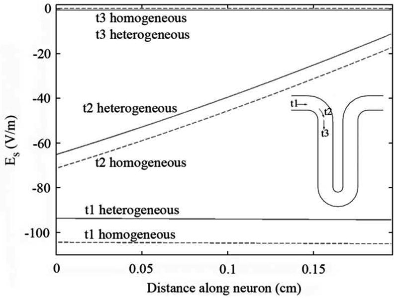
Effective electric field, E_s, along t interneurons, for a stimulator's output of 67 A/μs. The effective electric field in the heterogeneous model is represented by the solid line, while the effective electric field in the homogeneous model is represented by the dashed line. Distance is measured from the axon terminal towards the soma and the dendrite.

Figure 4.

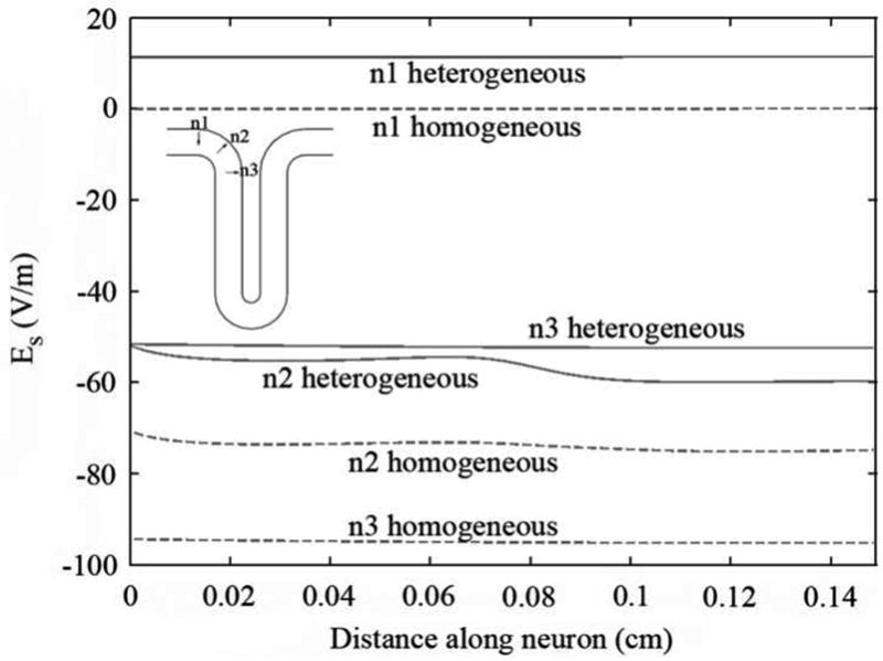
Effective electric field, E_s, along n interneurons, for a stimulator's output of 67 A/μs. The effective electric field in the heterogeneous model is represented by the solid line, while the effective electric field in the homogeneous model is represented by the dashed line. Distance is measured from the axon terminal towards the soma and the dendrite.

Regarding the effects of tissue heterogeneities on the effective field along cortical interneurons, we observed that the field induced at the interfaces (− ∇⃗ϕ) tended to oppose the field induced by the coil (−∂A⃗/∂t). This reduction was especially relevant for neurons lying perpendicular to the WM-GM interface (n neurons) for which the ratio between the homogeneous and heterogeneous effective electric field along them reached 1.8 (n3). For t neurons the reduction was smaller, with this ratio reaching a maximum value of only 1.1 for t1.

Contrary to the neurons mentioned above, the field along PTNs (Figure 5) and association fibers (Figure 6) varied considerably. One reason for this is that the axons of these neurons often bend sharply. Fiber bends gave rise to localized variations of the effective electric field due to a change in the orientation of the neurons relative to the coil. These effects are illustrated in Figure 5b, c and d (arrow 2), for PTNs, and in Figure 6a (arrows 2 and 6) and b (arrow 2), for association fibers. Another cause for the variability of E_s along these neurons is that they, unlike interneurons, often cross the WM-GM interface. The field due to charge accumulation at this interface creates a discontinuity in E_s (Miranda et al., 2007), which is shown in Figure 5b, c and d (arrow 3) and in Figure 6a (arrows 1 and 7) and b (arrow 1). Because charge accumulation depends on the existence of tissue heterogeneities, E_s in the homogeneous case lacked these discontinuities. Apart from these localized variations, E_s along the remaining sections of these neurons was relatively homogeneous, having high magnitudes if the section was aligned with the coil and close to it, and very low magnitudes when the section was perpendicular to the coil. An example of the latter is neuron P1, which is always perpendicular to the coil. The effective field along this neuron was very small, resulting only from charge accumulation at the interfaces. However, the electric field along the collateral of neuron P1 (see inset in Figure 5a) was very high due to the fact that it is parallel to the plane of the coil and located close to it, like neuron t1.

Figure 5.

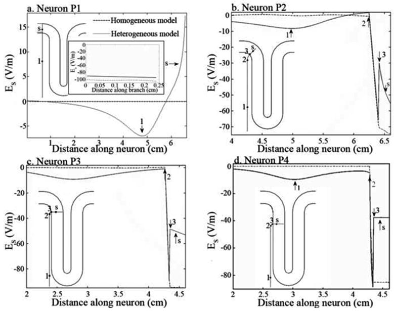
Effective electric field, E_s, along neurons P1-P4 (a-d) for both the homogeneous (dashed line) and heterogeneous models (solid line). The inset in (a) shows the effective electric field along the collateral of the axon of neuron P1. The effective electric field is shown at the time instant when it is maximum (maximum current time derivative of 67 A/μs). The arrows on the graphics indicate the most important features of E_s and the position of the soma (letter “s”). The position along the neuron where these features occur can be seen in the representation of the position of the neurons in the cortex that is shown in each figure.

Figure 6.

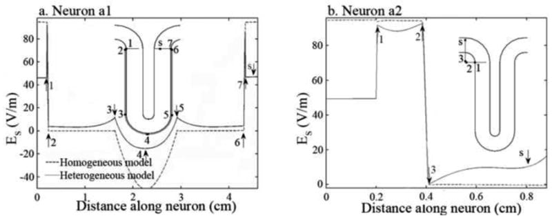
Effective electric field, E_s, along neurons a1 and a2 (a-b) for both the homogeneous (dashed line) and heterogeneous (solid line) models. The effective electric field is shown at the instant when it is a maximum (maximum time derivative of current of 67 A/μs). The insets show the neurons on their proper position in the cortex. The arrows on the graphics indicate the most important features of E_s (numbers) and the position of the soma (letter “s”). The position along the neuron where these features occur can be seen on the insets.

3.2. Activation sites and mechanisms

For cortical interneurons parallel to the electric field, stimulation always occurred at their axonal terminations. Stimulation at the dendritic end could never be achieved, because the polarization that occurred there had a faster spatial decay and a lower magnitude than at the axonal termination. This effect was not restricted to interneurons, but also applied to all the neurons modeled in this work. Stimulation of interneurons was, therefore, more easily achieved when the electric field induced in the tissue was directed along the dendrite-axon axis (PA direction for the neurons depicted in Figure 1c).

PTNs were always stimulated in the white matter, in the region where they bend after leaving the gray matter. This did not apply to neuron P1, which has no bends. When the electric field induced in the tissue was in the PA direction, the variation of E_s along the neuron (from axon to dendrite) due to the bend was negative, which caused a depolarization of the membrane. Therefore, stimulation occurred with lowest thresholds when the field pointed in this direction. The discontinuity in E_s that occurred at the WM-GM interface tended to induce a polarization that opposed the one induced at the fiber bend. In the case of the AP oriented electric field, the membrane was depolarized at the field discontinuity. However, because the hyperpolarization occurring at the nearby fiber bend had a higher magnitude, stimulation never occurred due to the “discontinuity mechanism”.

The collateral of neuron P1 was stimulated at its axonal termination by a PA-oriented electric field. The action potential generated at the termination propagated antidromically to the branching node but did not invade the main axon. The lack of propagation past the branching node is attributed to the large difference in fiber diameters, e.g., 6 μm for the collateral and 14 μm or 20 μm for the main axon. For this collateral diameter, propagation was observed only for main axon diameters less than 10 μm. When the electric field was directed along the AP direction, a depolarization occurred at the branching node. However, this was insufficient to stimulate the neuron, even at maximum stimulator output.

The case of association fibers was less straightforward. Due to their complex trajectories, these neurons possessed several sites where large changes in membrane polarization occurred, which lead to a competition among several stimulation mechanisms. Neuron a1 (Figure 6a) was stimulated at lower thresholds when the electric field was induced in the AP direction. However, stimulation sites depended on the diameter of the neurons. For smaller neurons (diameters between 6 μm and 12 μm) stimulation occurred at the axonal termination in the motor cortex. Larger neurons (14 μm to 20 μm) were stimulated more easily at the first fiber bend occurring after the neuron left the somatosensory cortex (arrows 6-7 in Figure 6a). This shift in activation site was due to the cancellation between the polarizations induced 1) at the fiber termination, in the motor cortex, and 2) at the last fiber bend, which occurs before entering the gray matter (arrows 1-2 in Figure 6a). Regarding neuron a2, it was also stimulated more easily by an AP directed electric field, which induced charge accumulation at its axonal termination.

3.3. Influence of pulse waveform and current direction on activation thresholds

As stated previously, cortical interneurons, PTNs and the collateral of neuron P1 were stimulated more easily when the electric field was induced in the PA direction. This occurred at different phases of the TMS waveform, depending on its type (monophasic or biphasic) and on the initial direction of the current in the coil. For monophasic PA pulses, stimulation occurred at the first phase of the waveform, whereas for monophasic AP pulses it only occurred in the second phase of the waveform. As the second phase is smaller than the first one, stimulation thresholds were much higher for AP than for PA pulses, by a factor of 2.7 to 2.8. Stimulation of these neurons with biphasic pulses was more easily attained with AP-PA pulses, at the second phase of the waveform as this was the only phase to induce a PA directed field. Thresholds for stimulation with this waveform type were even lower than thresholds for stimulation with monophasic PA pulses even though the magnitude of the first phase of the monophasic PA pulse is greater than the magnitude of the second phase of the biphasic AP-PA pulse. The ratio between thresholds for AP-PA pulses and for PA pulses varied between 0.7 and 0.9. For biphasic PA-AP pulses, stimulation occurred due to the sum of the depolarizations induced by the first and third phases of the pulse waveform. Contrary to what happened for AP-PA pulses, the thresholds for PA-AP pulses were about 1.1 times higher than those for monophasic PA pulses.

Since association fibers were most easily stimulated by AP directed electric fields, stimulation of these neurons occurred at waveform phases different from the ones where stimulation of the other modeled neurons occurred. Therefore, stimulation of association fibers with the lowest thresholds was always attained with biphasic PA-AP stimulation (at the second phase), followed by monophasic AP stimulation (at the first phase). Thresholds for biphasic AP-PA stimulation (third phase) were somewhat higher, and monophasic PA pulses (second phase) had the highest stimulation thresholds.

Table 1 summarizes the results presented thus far. Neurons not represented in the table (t2, t3 and n1) had very high stimulation thresholds and are not likely to be stimulated at all. The table shows that neuron a2 (for d₀ = 20 μm) had the lowest threshold of all neurons in the model, followed closely by the collateral of neuron P1 and by neuron t1 in the gyrus (for d₀ = 6 μm in both cases). Neurons P2 and P3 (d₀ = 20 μm) had similar stimulation thresholds, but higher than those of a2 and t1 neurons. Stimulation thresholds for neuron P4 were, on average, 18% higher than those for P3 (range: 13% - 26%). Neuron a1 had a threshold slightly higher than those of P2 and P3 but lower than that of P4. Neurons n2 and n3 both had thresholds higher than those of neuron P4. The diameter of the main axon of P1 had a negligible effect on the stimulation thresholds of the collateral.

Table 1.

Lowest stimulation thresholds for model PTNs (P2, P3, P4), cortical interneurons (t1, n2 and n3) and association fibers (a1, a2) as a function of waveform type. The table also shows the sites and mechanisms of activation and the phase of the waveform at which stimulation occurred.

Model Neuron (diameter)	Pulse type		Lowest threshold		Stimulation		Phase of waveformb
			A/μs	% of MSOa	Site	Mechanism
P2 (20 μm)	Mono	PA	97.7	57%	Axonal bend in white matter	Charge accumulation at the bend	1st 2nd 2nd 3rd
		AP	263.1	154%
	Bi	AP-PA	73.4	72%
		PA-AP	107.3	106%
P3 (20 μm)	Mono	PA	90.9	53%
		AP	252.9	148%
	Bi	AP-PA	70.7	70%
		PA-AP	98.4	97%
P4 (20 μm)	Mono	PA	105.9	62%
		AP	291.4	170%
	Bi	AP-PA	81.5	80%
		PA-AP	114.4	113%
Collateral of P1 (6 μm collateral, 20 μm main axon)	Mono	PA	64.8	38%	Collateral termination	Charge accumulation at axonal termination
		AP	165.5	97%
	Bi	AP-PA	48.2	47%
		PA-AP	72.2	71%
t1 (6μm)	Mono	PA	65.7	38%	Axonal termination (gray matter)	Charge accumulation at axonal termination
		AP	162.6	95%
	Bi	AP-PA	48.0	47%
		PA-AP	72.7	72%
n2 (6μm)	Mono	PA	116.7	68%
		AP	289.8	170%
	Bi	AP-PA	85.1	84%
		PA-AP	127.5	125%
n3 (6 μm)	Mono	PA	127.9	75%
		AP	318.1	186%
	Bi	AP-PA	93.4	92%
		PA-AP	139.7	137%
a1 (10 μm)	Mono	PA	171.7	101%	Axonal terminationc (gray matter, M1)	Charge accumulation at axonal	2nd 1st 3rd 2nd
		AP	104.8	61%
	Bi	AP-PA	106.7	105%
		PA-AP	79.1	78%
a2 (20 μm)	Mono	PA	70.2	41%
		AP	40.6	24%
	Bi	AP-PA	41.6	41%
		PA-AP	31.1	31%

^aAll values above 100 % for the Magstim 200 stimulator, and 120 % for the Magstim Rapid stimulator are outside the range of values that the stimulator can provide.

^bPhase of pulse waveform for which stimulation occurred. Each row corresponds to the pulse types displayed in the second column.

^cFor all pulse types, except monophasic PA, the threshold for activation at the bend after the fiber leaves the somato-sensory cortex was very similar to this one.

3.4. Effect of tissue heterogeneity and fiber diameter on activation sites and thresholds

The influence of tissue heterogeneity on activation sites was negligible. However, activation thresholds always increased due to the presence of these heterogeneities, with the magnitude of this increase varying from neuron to neuron. This was expected, since in this heterogeneous model of the cortex and surrounding tissues, the electric field is reduced inside the cortex and in the white matter, when compared to the field induced in an equivalent homogeneous model (Silva et al., 2008). The magnitude and direction of this effect is determined by the relative electrical conductivity values used for the brain tissues.

Regarding cortical interneurons, thresholds for activation tended to increase proportionally to the decrease of the field along the neuron. For neuron t1, for instance, the ratio between thresholds in the heterogeneous and homogeneous models (1.1) was the same as the ratio between effective electric fields in the two models. This was also the case for neuron n3 (ratio of 1.8), neuron t2 (ratio of 1.1), and there was also a very good agreement between the two ratios for neurons n2 (ratio of 1.3 between thresholds and 1.4 between the electric field).

For the other neuron types, tissue heterogeneities also resulted in increased thresholds. Regarding pyramidal tract neurons the ratio between thresholds was larger for neuron P4 (about 1.9) than for neurons P3 (about 1.7) and P2 (about 1.4). Finally, for association fibers, the thresholds increased more for neuron a1 (ratio of thresholds is about 2) than for neuron a2 (ratios between 1.1 and 1.4).

The influence of fiber diameter on activation sites was also negligible, except for neurons a1 and a2 (see section 3.2). As expected, the activation threshold was lowest for the largest diameter considered for the fiber, and these are the values reported in Table 1. The threshold for neuron a1 was the only exception due to the discussed shift in stimulation site with fiber diameter. For this neuron, the lowest threshold was obtained for a diameter of 10 μm.

4. Discussion

4.1. Mechanisms of stimulation and the site of activation

The dominant mechanism leading to neuronal activation and the site where it occurred varied substantially among the modeled neurons. The neurons modeling PTNs (P), for instance, were excited in the white matter where they bent (neuron P1 was an exception because it is straight and perpendicular to the coil). Cortical interneurons (n, t) and axon collaterals, on the other hand, were excited at their axonal terminations provided they were aligned with the main component of the field. Finally, pyramidal association fibers (a) were stimulated either at their axonal termination or at some sharp axonal bend. These results highlight the importance of fiber bends and axonal terminations in stimulation of motor cortical neurons, as has been suggested in other studies (Nagarajan et al., 1993; Maccabee et al., 1998). Geometrical factors such as these can create very strong and localized variations of the effective electric field along the neuron, even when the gradient of the field induced by the coil is small.

The overall effectiveness of stimulation at axonal terminations was much greater than that of stimulation at fiber bends, a well-known result from cable theory (Roth, 1994). This was illustrated by the much lower activation thresholds of cortical interneurons as compared to PTNs, even though the diameters of the former (maximum of 6 μm) were much smaller than those of the latter (maximum of 20 μm). Also in agreement with theoretical predictions was the fact that thresholds for stimulation by these mechanisms were proportional to the strength of E_s along the neuron (Roth, 1994). This was shown by the fact that the ratio between the homogeneous and the heterogeneous effective electric fields along cortical interneurons was equal to the ratio between the activation thresholds for the homogeneous and the heterogeneous models.

Apart from the two aforementioned stimulation mechanisms, another stimulation mechanism also influenced the activation thresholds. This can be seen by comparing the response of P neurons to homogeneous and heterogeneous effective electric fields. The homogeneous effective field differs from the heterogeneous one essentially by the absence of the field discontinuity (arrow 3 in Figure 5b-d). However, stimulation thresholds were smaller for the homogeneous model, indicating that the discontinuities in E_s diminished the effectiveness of stimulation at fiber bends, even though the latter remained the dominant stimulation mechanism. This effect strengthens the importance of modeling tissue heterogeneities, as has been stressed previously by others (Kobayashi et al., 1997; Maccabee et al., 1991; Miranda et al., 2003; Miranda et al., 2007; Silva et al., 2008).

The influence of fiber branching in neuronal stimulation was also considered, through the inclusion of one horizontal axon collateral in neuron P1. A change in polarization did occur at the branching node, but with opposite sign and smaller magnitude than the change occurring at the collateral's termination. The lower excitability of branches compared to terminations is also in agreement with theoretical predictions (Roth, 1994). Increasing the diameter of the axon collateral or decreasing its length would lead to a greater interaction between these two polarizations changes, which could make stimulation at the termination less effective.

4.2. Comparison with experimental results

In this model, monophasic PA stimulation of medium caliber cortical interneurons and axon collaterals (6 μm diameter), located at the top of the gyrus and parallel to the WM-GM interface, was achieved at 65.7 A/μs and 64.9 A/μs, respectively. These values lie within the range of experimental values reported in the literature for I-wave generation: 43.5 – 67.1 A/μs (Di Lazzaro et al., 1998; Di Lazzaro et al., 2001a; Kammer et al., 2001). These thresholds are lower than those obtained here for stimulation of large PTNs located near the lip of the gyrus, for which the minimum threshold, 90.9 A/μs, lies in the range of values reported in the literature for D-wave generation: 82.1-91.2 A/μs (Di Lazzaro et al., 1998; Di Lazzaro et al., 2004). Analyzing these thresholds in terms of an average resting motor threshold (RMT), 67 A/μs according to (Kammer et al., 2001), we see that interneurons and axon collaterals could be stimulated at RMT, while stimulation of PTNs could not be achieved below 134% RMT (neuron P3). Neuron P4 could only be stimulated at 158% RMT. Therefore, at RMT, no PTN could be stimulated, but at 150% RMT stimulation of PTNs could be achieved possibly up to a depth of 8 mm from the cortical surface (neuron P4), or 2.8 cm from the scalp, in our model, but no further than that.

These results are in better agreement with experimental data than our previous modeling study (Silva et al., 2008), which predicted direct stimulation of large caliber PTNs under a monophasic PA stimulus at RMT, although in that case a different model for the neuronal membrane was assumed (Basser and Roth, 1991).

Still under PA monophasic stimulation, neuron a2 could be stimulated at thresholds close to the ones obtained for cortical interneurons: 70.2 A/μs (about 41.1% of MSO) for d₀ = 20 μm. Again, this is close to the threshold range for I-wave generation reported experimentally. However, given that these neurons do not project as far as PTNs do, it seems unlikely that they have such large diameters (Manola et al., 2007). If we considered smaller diameters, the thresholds would increase to values between those of cortical interneurons and PTNs.

Regarding monophasic AP stimulation, our results indicated that cortical interneurons modeled in this work could not be stimulated at thresholds achievable with TMS devices used today. This was a direct consequence of i) the specific orientation chosen for the horizontally aligned cortical interneurons in the model, i.e., dendrite posterior to axon, and ii) the difficulty in stimulating the apical dendrite. Reversing this orientation would cause thresholds for AP stimulation to be similar to ones obtained for PA stimulation. The distribution of orientations of horizontal interneurons is possibly isotropic, but no evidence could be found in the literature of the actual orientation pattern.

Still regarding monophasic AP pulses, PTNs also could not be stimulated at thresholds within operating range of TMS devices; with this direction of the current, PTNs were strongly hyperpolarized at their bending site, during the first phase of the pulse waveform. In this case, depolarization only occurred during the second phase of the waveform, which has a much smaller magnitude. However, during AP stimulation, D-waves have been reported (Di Lazzaro et al., 2001a). This could be a result of stimulation of PTNs from other cortical areas, like the somatosensory cortex or premotor and supplementary motor areas. PTNs from these areas, as opposed to what happened with PTNs emanating from M1, have their bends oriented in such a way that they are depolarized with an AP oriented field and hyperpolarized with PA oriented fields. Yet, stimulation of PTNs from the somatosensory cortex was shown not to elicit a motor response (Di Lazzaro et al., 2008). Moreover, such neurons are thought to have small diameters (in the 2-4 μm range; McComas and Wilson 1968) and are therefore very difficult to stimulate, according to the results presented in this work. To the best of our knowledge, no similar information is available regarding the fibers emanating from the premotor and supplementary motor areas and, therefore, they might be a possible source for D-wave generation with an AP oriented field.

Experimental studies (Kammer et al., 2001; Di Lazzaro et al., 2004; Sakai et al., 1997; Mills et al., 1992) have reported that monophasic AP stimulation has a higher threshold than PA stimulation, and that it gives rise to a longer latency I-wave (I₃-wave). Several works have attributed the difference in thresholds between PA and AP stimulation as a consequence of the latter stimulating a different population of neurons, other than cortical interneurons (Di Lazzaro et al., 2004; Sakai et al., 1997). Esser et al. (Esser et al., 2005) have suggested that association fibers may be responsible for the different outcomes of AP and PA stimulation. There, the authors presented simulations that showed that stimulation of fibers projecting from the somatosensory cortex to the motor cortex, at the site where the fibers bend into the motor cortex, led to a wave with the same latency as an I₃-wave. Our results suggest that pyramidal association fibers (neurons a1 and a2) have thresholds for monophasic AP stimulation much smaller than those for PA stimulation. The stimulation of neurons a1/a2 can only give rise to an indirect (I) wave, so this could be the possible source of late I waves under AP stimulation. Neuron a2 is especially relevant, given that its thresholds – ranging between 111.8 A/μs and 40.6 A/μs for fiber diameters between 6 μm and 20 μm, respectively – are in good agreement with experimental measurements of thresholds for AP stimulation (values between 59.7 A/μs and 99 A/μs, (Di Lazzaro et al., 2001a; Kammer et al., 2001)). Neuron a1, which represents the type of fibers identified by Esser et al. as giving rise to the late I-wave, had stimulation thresholds somewhat higher than those observed experimentally, with values between 104.8 A/μs and 137.9 A/μs. Still regarding Esser's work it should be noted that we disagree as to where stimulation occurs. Our present work shows that an AP pulse would hyperpolarize association fibers projecting from the somatosensory cortex (a1) in the region where it bends into the motor cortex. Stimulation of these association fibers with AP pulses always occurred at the fiber terminal in layer III of the motor cortex.

Finally, biphasic pulses always stimulated neurons during the second or third phase of the waveform, depending on the type of neuron and initial direction of the current in the coil. For pyramidal tract neurons and cortical interneurons, activation with biphasic AP-PA pulses occurred during the second phase of the waveform (the only one that induced a PA directed electric field), at thresholds lower than those necessary for stimulation with monophasic PA pulses (in terms of the maximum value of the current's time derivative). The increased efficiency of the second phase predicted here is in good agreement with results reported by others (Kammer et al., 2001; Maccabee et al., 1998), who attribute it to the fact that the second phase of the waveform lasts twice as long as the first phase of a monophasic pulse, rendering it more effective.

4.3. Generation of D and I-waves

D-waves are attributed to the direct stimulation of the axons of PTNs. According to our model these might be large PTNs located near the lip of the gyrus. I-waves, on the other hand, result from a complex interaction between cortical cells of different types (Ziemann and Rothwell, 2000; Esser et al., 2005). Even though the present study concerns only single cell stimulation, the results may tell us something about the initial steps involved in the generation of these waves. It is possible that stimulation of both interneurons and axon collaterals of PTNs could contribute to the generation of I-waves, since both are recruited at RMT and since it is likely that both excitatory and inhibitory input is necessary to generate I-waves (Esser et al., 2005). In particular, stimulation of PTN axon collaterals alone is not sufficient to generate I-waves (Patton and Amassian, 1954). Local connections between PTNs are provided both by PTN axon collaterals and interneurons (Somogyi et al., 1998). Given that PTNs are excitatory cells and the majority of interneurons are inhibitory (Markram et al., 2004), stimulation of the synaptic terminals of the axon collaterals of PTNs could elicit the excitatory drive needed to generate the I-waves, whereas stimulation of interneurons could elicit the inhibitory drive. Smaller pyramidal cells are unlikely to be stimulated at threshold. Furthermore, the fact that in our model the action potential elicited at the termination of the axon collateral always failed to invade the main axon of the PTN might also explain why stimulation of these axon collaterals is possible without eliciting a D-wave. Antidromic propagation in branched axons has been described in the context of deep brain stimulation (Grill et al., 2008), but the range of axon diameters modeled were quite different from those of PTNs.

4.4. Model limitations and future work

One of the main limitations of this work is that accurate mathematical models describing the active membrane properties of cortical neurons are still unavailable. The model used in this work is based on data obtained from human myelinated sensory fibers (Wesselink et al., 1999), which may not be appropriate to describe the three kinds of neurons modeled in this work. Additionally, data regarding the diameters of the fibers modeled here are still lacking, except for pyramidal tract neurons (Lassek, 1940). These two factors may significantly affect the stimulation thresholds reported here.

Another important limitation lies in the approximate geometry of the central sulcus modeled in this work. In fact, it has been shown that the hand-area of the motor cortex has a “hook” shape when viewed in a parasagittal plane (Yousry et al., 1997), unlike the straight vertical wall modeled here. Despite this, our model is a good approximation of the upper part of the central sulcus, close to the lip of the gyrus, where the majority of the TMS-recruited neurons are thought to be. For deeper parts the model fails, but neurons there are less affected by the field induced by TMS. On the other hand, the characteristic “hook” shape of the sulcus affects the paths taken by the axons of PTNs. This may cause the axonal bends to be less sharp, and consequently a lower depolarization to be elicited there. In this case, PTNs could be stimulated by a mechanism other than the axonal bend, such as the field discontinuity at the WM/GM interface. Therefore, the exact mechanism activating a PTN will depend on the specific combination of all these factors.

The simplified geometry of this sulcus model also prevents it from being used to study LM simulation. The latter form of stimulation has been shown to yield results significantly different from those of either AP or PA stimulation (Di Lazzaro et al., 2001a), which is probably due to the Ω shape of the hand-area of the motor cortex when viewed in an axial plane (Yousry et al., 1997). As this shape was not modeled in the present work, the results of LM stimulation cannot be inferred from the current ones.

The fact that the present model does not account for the Ω shape should, however, have a limited effect on the results obtained for PA / AP stimulation. This is strengthened by the work of Herbsman et al. (2009), which shows the absence of correlation between the motor threshold and the component of the diffusion tensor along the LM direction under an AP monophasic pulse (Herbsman et al., 2009). This suggests that mainly the neurons present in the part of the hand knob perpendicular to the AP electric field were being recruited. In other words, for AP or PA stimulation, our model contains the relevant region of the hand knob, which is the section perpendicular to the electric field. However, the existence of an Ω-shaped knob in a real brain would affect the electric field magnitude and hence the estimated threshold values.

Also, it is known that background cortical activity changes the cortical excitability and the individual stimulation thresholds (Matthews, 1999), and our model does not contemplate that.

It should also be stressed that the findings reported in this work refer to single pulse TMS and should not be extrapolated to studies involving repetitive stimulation of the motor cortex (rTMS). rTMS of the motor cortex has been shown to lead to a spread of the activation to muscles far from the target area, and to influence cortical excitability (Terao and Ugawa, 2002; Di Lazzaro et al, 2008). These effects depend most likely on the effects of rTMS on synapses between cortical neurons (Di Lazzaro et al, 2008) and, therefore, cannot by accounted for in the present model. For the same reason, results obtained with paired-pulse paradigms (Di Lazzaro et al, 2008) are also outside the scope of this work.

Given the limitations pointed out above, and despite the good agreement between the modeling results and the experimental data, the conclusions outlined in this discussion should be confirmed using more accurate models. An important improvement would be to use high-resolution human head models that include a detailed 3D description of the geometry of the cortical sheet (e.g. Chen and Mogul, 2009). This would increase the accuracy of the calculation of the electric field and would help to describe in a more realistic way the trajectory of the neuron in the field. Additionally, a more accurate representation of the neuronal geometry that includes the main features of the axonal arborization would, in conjunction with better data for the electrophysiological properties of the neurons, lead to better estimates of the changes in membrane potential. Finally, the model could be improved by including simulations of synaptic connections between the several neurons represented. That would allow us not only to investigate the mechanisms that determine stimulation of an individual neuron, but also to predict the response due to synaptic interactions between neurons in the network.

4.5. Concluding remarks

In this work the electric field induced by a figure-eight coil along neurons embedded in an idealized model of the human motor cortex was calculated. The response of the neurons following a TMS stimulus was predicted by taking into account the spatial and temporal variations of the electric field induced by the coil, the effects of tissue heterogeneities, and the influence of the neuron's position, orientation and geometry. This model allowed us to predict the influence of these factors on the recruitment order of neurons in the motor cortex, on their activation thresholds, and on the activation site. Despite some limitations inherent to this model, most of its predictions are consistent with experimental results and offer some insights into the possible origin of the responses elicited by TMS of the motor cortex.

References

- Amassian VE, Eberle L, Maccabee PJ, Cracco RQ. Modelling magnetic coil excitation of human cerebral cortex with a peripheral nerve immersed in a brain-shaped volume conductor: the significance of fiber bending in excitation. Electroencephalogr Clin Neurophysiol. 1992;85:291–301. doi: 10.1016/0168-5597(92)90105-k. [DOI] [PubMed] [Google Scholar]
- Basser PJ, Roth BJ. Stimulation of a myelinated nerve axon by electromagnetic induction. Med Biol Eng Comput. 1991;29:261–8. doi: 10.1007/BF02446708. [DOI] [PubMed] [Google Scholar]
- Brodal P. The central nervous system: Structure and function. 2nd. Oxford University Press Inc; 1998. [Google Scholar]
- Chen M, Mogul DJ. A structurally detailed finite element human head model for simulation of transcranial magnetic stimulation. J Neurosci Methods. 2009;179:111–20. doi: 10.1016/j.jneumeth.2009.01.010. [DOI] [PubMed] [Google Scholar]
- Day BL, Dressler D, Denoordhout AM, Marsden CD, Nakashima K, Rothwell JC, et al. Electric and magnetic stimulation of human motor cortex - surface EMG and single motor unit responses. J Physiol. 1989;412:449–73. doi: 10.1113/jphysiol.1989.sp017626. [DOI] [PMC free article] [PubMed] [Google Scholar]
- De Lucia M, Parker GJ, Embleton K, Newton JM, Walsh V. Diffusion tensor MRI-based estimation of the influence of brain tissue anisotropy on the effects of transcranial magnetic stimulation. Neuroimage. 2007;36:1159–70. doi: 10.1016/j.neuroimage.2007.03.062. [DOI] [PubMed] [Google Scholar]
- Di Lazzaro V, Oliviero A, Mazzone P, Insola A, Pilato F, Saturno E, et al. Comparison of descending volleys evoked by monophasic and biphasic magnetic stimulation of the motor cortex in conscious humans. Exp Brain Res. 2001a;141:121–7. doi: 10.1007/s002210100863. [DOI] [PubMed] [Google Scholar]
- Di Lazzaro V, Oliviero A, Pilato F, Saturno E, Dileone M, Mazzone P, et al. The physiological basis of transcranial motor cortex stimulation in conscious humans. Clin Neurophysiol. 2004;115:255–66. doi: 10.1016/j.clinph.2003.10.009. [DOI] [PubMed] [Google Scholar]
- Di Lazzaro V, Oliviero A, Profice P, Meglio M, Cioni B, Tonali P, et al. Descending spinal cord volleys evoked by transcranial magnetic and electrical stimulation of the motor cortex leg area in conscious humans. J Physiol. 2001b;537:1047–58. doi: 10.1111/j.1469-7793.2001.01047.x. [DOI] [PMC free article] [PubMed] [Google Scholar]
- Di Lazzaro V, Oliviero A, Profice P, Saturno E, Pilato F, Insola A, et al. Comparison of descending volleys evoked by transcranial magnetic and electric stimulation in conscious humans. Electroencephalogr Clin Neurophysiol. 1998;109:397–401. doi: 10.1016/s0924-980x(98)00038-1. [DOI] [PubMed] [Google Scholar]
- Di Lazzaro V, Ziemann U, Lemon RN. State of the art: Physiology of transcranial motor cortex stimulation. Brain Stimulation. 2008;1:345–62. doi: 10.1016/j.brs.2008.07.004. [DOI] [PubMed] [Google Scholar]
- Esser SK, Hill SL, Tononi G. Modeling the effects of transcranial magnetic stimulation on cortical circuits. J Neurophysiol. 2005;94:622–39. doi: 10.1152/jn.01230.2004. [DOI] [PubMed] [Google Scholar]
- Foust A, Popovic M, Zecevic D, McCormick DA. Action Potentials Initiate in the Axon Initial Segment and Propagate through Axon Collaterals Reliably in Cerebellar Purkinje Neurons. J Neurosci. 2010;30:6891–6902. doi: 10.1523/JNEUROSCI.0552-10.2010. [DOI] [PMC free article] [PubMed] [Google Scholar]
- Fox PT, Narayana S, Tandon N, Sandoval H, Fox SP, Kochunov P, et al. Column-based model of electric field excitation of cerebral cortex. Hum Brain Mapp. 2004;22:1–14. doi: 10.1002/hbm.20006. [DOI] [PMC free article] [PubMed] [Google Scholar]
- Ghosh S, Porter R. Morphology of pyramidal neurones in monkey motor cortex and the synaptic actions of their intracortical axon collaterals. J Physiol. 1988;400:593–615. doi: 10.1113/jphysiol.1988.sp017138. [DOI] [PMC free article] [PubMed] [Google Scholar]
- Grill WM, Cantrell MB, Robertson MS. Antidromic propagation of action potentials in branched axons: implications for the mechanisms of action of deep brain stimulation. J Comput Neurosci. 2008;24:81–93. doi: 10.1007/s10827-007-0043-9. [DOI] [PubMed] [Google Scholar]
- Hines M. Efficient computation of branched nerve equations. Int J Biomed Comput. 1984;15:69–76. doi: 10.1016/0020-7101(84)90008-4. [DOI] [PubMed] [Google Scholar]
- Herbsman T, Forster L, Molnar C, Dougherty R, Christie D, Koola J, Ramsey D, Morgan PS, Bohning DE, George MS, Nahas Z. Motor threshold in transcranial magnetic stimulation: the impact of white matter fiber orientation and skull-to-cortex distance. Hum Brain Mapp. 2009;30:2044–55. doi: 10.1002/hbm.20649. [DOI] [PMC free article] [PubMed] [Google Scholar]
- Hongo T, Kudo N, Sasaki S, Yamashita M, Yoshida K, Ishizuka N, et al. Trajectory of group Ia and Ib fibers from the hind-limb muscles at the L3 and L4 segments of the spinal cord of the cat. J Comp Neurol. 1987;262:159–94. doi: 10.1002/cne.902620202. [DOI] [PubMed] [Google Scholar]
- Kammer T, Beck S, Thielscher A, Laubis-Herrmann U, Topka H. Motor thresholds in humans: a transcranial magnetic stimulation study comparing different pulse waveforms, current directions and stimulator types. Clin Neurophysiol. 2001;112:250–8. doi: 10.1016/s1388-2457(00)00513-7. [DOI] [PubMed] [Google Scholar]
- Kammer T, Vorwerg M, Herrnberger B. Anisotropy in the visual cortex investigated by neuronavigated transcranial magnetic stimulation. Neuroimage. 2007;36:313–21. doi: 10.1016/j.neuroimage.2007.03.001. [DOI] [PubMed] [Google Scholar]
- Kobayashi M, Ueno S, Kurokawa T. Importance of soft tissue inhomogeneity in magnetic peripheral nerve stimulation. Electroencephalogr Clin Neurophysiol. 1997;105:406–13. doi: 10.1016/s0924-980x(97)00035-0. [DOI] [PubMed] [Google Scholar]
- Lassek AM. The human pyramidal tract II A numerical investigation of the Betz cells of the motor area. Arch Neurol Psychiatry. 1940;44:718–24. [Google Scholar]
- Maccabee PJ, Amassian VE, Eberle LP, Cracco RQ. Magnetic coil stimulation of straight and bent amphibian and mammalian peripheral nerve in vitro: locus of excitation. J Physiol. 1993;460:201–19. doi: 10.1113/jphysiol.1993.sp019467. [DOI] [PMC free article] [PubMed] [Google Scholar]
- Maccabee PJ, Amassian VE, Eberle LP, Rudell AP, Cracco RQ, Lai KS, et al. Measurement of the electric-field induced into inhomogeneous volume conductors by magnetic coils - Application to human spinal neurogeometry. Electroencephalogr Clin Neurophysiol. 1991;81:224–37. doi: 10.1016/0168-5597(91)90076-a. [DOI] [PubMed] [Google Scholar]
- Maccabee PJ, Nagarajan SS, Amassian VE, Durand DM, Szabo AZ, Ahad AB, et al. Influence of pulse sequence, polarity and amplitude on magnetic stimulation of human and porcine peripheral nerve. J Physiol. 1998;513:571–85. doi: 10.1111/j.1469-7793.1998.571bb.x. [DOI] [PMC free article] [PubMed] [Google Scholar]
- Manola L, Roelofsen BH, Holsheimer J, Marani E, Geelen J. Modelling motor cortex stimulation for chronic pain control: electrical potential field, activating functions and responses of simple nerve fibre models. Med Biol Eng Comput. 2005;43:335–43. doi: 10.1007/BF02345810. [DOI] [PubMed] [Google Scholar]
- Manola L, Holsheimer J, Veltink P, Buitenweg JR. Anodal vs cathodal stimulation of motor cortex: a modeling study. Clin Neurophysiol. 2007;118:464–74. doi: 10.1016/j.clinph.2006.09.012. [DOI] [PubMed] [Google Scholar]
- Markram H, Toledo-Rodriguez M, Wang Y, Gupta A, Silberberg G, Wu C. Interneurons of the neocortical inhibitory system. Nat Rev Neurosci. 2004;5:793–807. doi: 10.1038/nrn1519. [DOI] [PubMed] [Google Scholar]
- Mascagni MV. Numerical methods for neuronal modeling. In: Koch C, Segev I, editors. Methods in neuronal modeling: from ions to networks. 2nd. Cambridge: MA: MIT press; 1998. [Google Scholar]
- Matthews PB. The effect of firing on the excitability of a model motoneurone and its implications for cortical stimulation. J Physiol. 1999;518:867–82. doi: 10.1111/j.1469-7793.1999.0867p.x. [DOI] [PMC free article] [PubMed] [Google Scholar]
- McComas AJ, Wilson P. An investigation of pyramidal tract cells in the somatosensory cortex of the rat. J Physiol. 1968;194:271–88. doi: 10.1113/jphysiol.1968.sp008407. [DOI] [PMC free article] [PubMed] [Google Scholar]
- Meyer G. Forms and Spatial Arrangement of Neurons in the Primary Motor Cortex of Man. J Comp Neurol. 1987;262:402–28. doi: 10.1002/cne.902620306. [DOI] [PubMed] [Google Scholar]
- Mills KR, Boniface SJ, Schubert M. Magnetic brain-stimulation with a double coil - the importance of coil orientation. Electroencephalogr Clin Neurophysiol. 1992;85:17–21. doi: 10.1016/0168-5597(92)90096-t. [DOI] [PubMed] [Google Scholar]
- Miranda PC, Correia L, Salvador R, Basser PJ. Tissue heterogeneity as a mechanism for localized neural stimulation by applied electric fields. Phys Med Biol. 2007;52:5603–17. doi: 10.1088/0031-9155/52/18/009. [DOI] [PubMed] [Google Scholar]
- Miranda PC, Hallett M, Basser PJ. The electric field induced in the brain by magnetic stimulation: A 3-D finite-element analysis of the effect of tissue heterogeneity and anisotropy. IEEE Trans Biomed Eng. 2003;50:1074–85. doi: 10.1109/TBME.2003.816079. [DOI] [PubMed] [Google Scholar]
- Nagarajan SS, Durand DM, Warman EN. Effects of induced electric fields on finite neuronal structures - a simulation study. IEEE Trans Biomed Eng. 1993;40:1175–88. doi: 10.1109/10.245636. [DOI] [PubMed] [Google Scholar]
- Nilsson J, Panizza M, Roth BJ, Basser PJ, Cohen LG, Caruso G, et al. Determining the site of stimulation during magnetic stimulation of a peripheral nerve. Electroencephalogr Clin Neurophysiol. 1992;85:253–64. doi: 10.1016/0168-5597(92)90114-q. [DOI] [PubMed] [Google Scholar]
- Patton HD, Amassian VE. Single-unit and multiple-unit analysis of cortical stage of pyramidal tract activation. J Neurophysiol. 1954;17:345–63. doi: 10.1152/jn.1954.17.4.345. [DOI] [PubMed] [Google Scholar]
- Roth BJ. Mechanisms for electrical stimulation of excitable tissue. Crit Rev Biomed Eng. 1994;22:253–305. [PubMed] [Google Scholar]
- Roth BJ, Basser PJ. A model of the stimulation of a nerve fiber by electromagnetic induction. IEEE Trans Biomed Eng. 1990;37:588–97. doi: 10.1109/10.55662. [DOI] [PubMed] [Google Scholar]
- Rothwell JC. Techniques and mechanisms of action of transcranial stimulation of the human motor cortex. J Neurosci Methods. 1997;74:113–22. doi: 10.1016/s0165-0270(97)02242-5. [DOI] [PubMed] [Google Scholar]
- Sakai K, Ugawa Y, Terao Y, Hanajima R, Furubayashi T, Kanazawa I. Preferential activation of different I waves by transcranial magnetic stimulation with a figure-of-eight-shaped coil. Exp Brain Res. 1997;113:24–32. doi: 10.1007/BF02454139. [DOI] [PubMed] [Google Scholar]
- Silva S, Basser PJ, Miranda PC. Elucidating the mechanisms and loci of neuronal excitation by transcranial magnetic stimulation using a finite element model of a cortical sulcus. Clin Neurophysiol. 2008;119:2405–13. doi: 10.1016/j.clinph.2008.07.248. [DOI] [PMC free article] [PubMed] [Google Scholar]
- Somogyi P, Tamás G, Lujan R, Buhl EH. Salient features of synaptic organization in the cerebral cortex. Brain Res Rev. 1998;26:113–35. doi: 10.1016/s0165-0173(97)00061-1. [DOI] [PubMed] [Google Scholar]
- Standring S. Gray's Anatomy: The Anatomical Basis of Clinical Practice. 39th. Elsevier Churchill Livingstone; 2004. [Google Scholar]
- Struijk JJ, Holsheimer J, van der Heide GG, Boom HB. Recruitment of dorsal column fibers in spinal cord stimulation: influence of collateral branching. IEEE Trans Biomed Eng. 1992;39:903–12. doi: 10.1109/10.256423. [DOI] [PubMed] [Google Scholar]
- Tasaki I. New measurements of the capacity and the resistance of the myelin sheath and the nodal membrane of the isolated frog nerve fiber. Am J Physiol. 1955;181:639–50. doi: 10.1152/ajplegacy.1955.181.3.639. [DOI] [PubMed] [Google Scholar]
- Terao Y, Ugawa Y. Basic mechanisms of TMS. J Clin Neurophysiol. 2002;19:322–43. doi: 10.1097/00004691-200208000-00006. [DOI] [PubMed] [Google Scholar]
- Thielscher A, Kammer T. Linking physics with physiology in TMS: A sphere field model to determine the cortical stimulation site. TMS Neuroimage. 2002;17:1117–30. doi: 10.1006/nimg.2002.1282. [DOI] [PubMed] [Google Scholar]
- Thielscher A, Kammer T. Electric field properties of two commercial figure-8 coils in TMS: calculation of focality and efficiency. Clin Neurophysiol. 2004;115:1697–1708. doi: 10.1016/j.clinph.2004.02.019. [DOI] [PubMed] [Google Scholar]
- Tsugorka T, Dovgan' O, Stepanyuk A, Cherkas V. Variety of types of cortical interneurons. Neurophysiology. 2007;39:227–36. [Google Scholar]
- Wang Y, Gupta A, Toledo-Rodriguez M, Wu CZ, Markram H. Anatomical, physiological, molecular and circuit properties of nest basket cells in the developing somatosensory cortex. Cereb Cortex. 2002;12:395–410. doi: 10.1093/cercor/12.4.395. [DOI] [PubMed] [Google Scholar]
- Warman EN, Grill WM, Durand D. Modeling the effects of electric fields on nerve fibers: determination of excitation thresholds. IEEE Trans Biomed Eng. 1992;39:1244–54. doi: 10.1109/10.184700. [DOI] [PubMed] [Google Scholar]
- Wesselink WA, Holsheimer J, Boom HBK. A model of the electrical behaviour of myelinated sensory nerve fibres based on human data. Med Biol Eng Comput. 1999;37:228–35. doi: 10.1007/BF02513291. [DOI] [PubMed] [Google Scholar]
- Yamashita A, Arikuni T. Axon trajectories in local circuits of the primary motor cortex in the macaque monkey (Macaca fuscata) Neurosci Res. 2001;39:233–45. doi: 10.1016/s0168-0102(00)00220-0. [DOI] [PubMed] [Google Scholar]
- Yousry TA, Schmid UD, Alkadhi H, Schmidt D, Peraud A, Buettner A, et al. Localization of the motor hand-area to a knob on the precentral gyrus - A new landmark. Brain. 1997;120:141–57. doi: 10.1093/brain/120.1.141. [DOI] [PubMed] [Google Scholar]
- Ziemann U, Rothwell JC. I-waves in motor cortex. J Clin Neurophysiol. 2000;17:397–405. doi: 10.1097/00004691-200007000-00005. [DOI] [PubMed] [Google Scholar]