Performing Real-Time Interactive Fiber Tracking

Abstract

Fiber tracking is a technique that, based on a diffusion tensor magnetic resonance imaging dataset, locates the fiber bundles in the human brain. Because it is a computationally expensive process, the interactivity of current fiber tracking tools is limited. We propose a new approach, which we termed real-time interactive fiber tracking, which aims at providing a rich and intuitive environment for the neuroradiologist. In this approach, fiber tracking is executed automatically every time the user acts upon the application. Particularly, when the volume of interest from which fiber trajectories are calculated is moved on the screen, fiber tracking is executed, even while it is being moved. We present our fiber tracking tool, which implements the real-time fiber tracking concept by using the video card’s graphics processing units to execute the fiber tracking algorithm. Results show that real-time interactive fiber tracking is feasible on computers equipped with common, low-cost video cards.

Electronic supplementary material

The online version of this article (doi:10.1007/s10278-009-9266-9) contains supplementary material, which is available to authorized users.

Introduction

Diffusion tensor magnetic resonance imaging (DT-MRI) is a technique that, given a set of magnetic resonance scans acquired with a specific protocol, allows the estimation of diffusion tensors at all voxels of the volume.^1,2 Most commonly, the human brain is imaged,³ although other structures, like the spinal cord, have been imaged as well.⁴ The diffusion tensor is a mathematical model that bears information on both the direction and the intensity of diffusion. In the context of DT-MRI, it characterizes the diffusion of water molecules along myelinated neuronal fibers.⁵

The post-processing of DT-MRI volumes typically consists of the fiber tracking process, which takes advantage of the information on water diffusion to determine the locations of fiber bundles.^6,7 There are several fiber tracking techniques,^8–10 one of them being the streamline method,¹¹ which finds fiber trajectories by following the main diffusion direction of water. Heuristics may be used to further improve the quality of results and to solve problems related to partial volume effects,¹² such as fiber crossing or fiber kissing. Streamline fiber tracking, with which this article is concerned, is typically executed for a given volume of interest (VOI), where seed points are evenly spread and each of which generates a fiber trajectory. This method of fiber tracking relies on mathematical operations like vector integration and interpolation.¹³

The large number of complex mathematical operations that the fiber tracking process requires hinders the interactivity provided by applications, since a significant amount of time is spent on those operations. To the best of our knowledge, current commercial systems cope with the processing time issues either by not allowing interactive fiber tracking at all or by requiring the result of a full-brain fiber tracking process to be loaded prior to being explored. One commercial product, the iPlan BOLD MRI Mapping software from BrainLAB,¹⁴ provides interactive fiber tracking, but sets of precomputed trajectories are required to be loaded beforehand into the program for exploratory actions to be taken. Another commercial product, the BrainVoyager QX,^15–17 on the other hand, does not need precalculated trajectories to be loaded before exploration, but the interactivity experienced by the user is not as rich as that provided by iPlan BOLD MRI Mapping.

In order to speed up the process of fiber tracking, the use of graphics processing units (GPUs) has been proposed. Jeong et al.¹⁸ have proposed the use of GPUs to compute and visualize white matter connectivity by means of a voxel-based approach. Petrovic et al.¹⁹ have used GPUs in order to visualize fiber tracking results, which are not generated by the GPU in their approach. McGraw and Nadar²⁰ have shown how stochastic fiber tracking can be executed on the GPU, allowing the user to observe results being generated on the screen. We have previously proposed the use of GPUs for the execution of streamline fiber tracking²¹ and have also compared them with computer clusters in this context²². An optimized strategy for performing fiber tracking on GPUs was later proposed by Köhn et al.,²³ who employed geometry shaders to calculate results. Kwatra et al.²⁴ have proposed the use of programmable hardware for fiber tracking, but this approach has the inconvenience of using non-standard hardware, whereas the GPU approaches require only a consumer-grade graphics card.

In this article, we present a novel approach to interactivity in the context of fiber tracking, which we have termed real-time interactive fiber tracking. In this approach, the user can interactively define VOIs, move them around the DT-MRI volume, change the fiber tracking algorithm’s parameters, and have all results calculated in real time, while interaction occurs. When the user moves the VOI to a new position, for instance, new fibers are calculated automatically and quickly, even while the VOI is being dragged, thus producing an animation-like effect. This approach introduces a whole new level of interactivity, in which the user neither has to preload previous fiber tracking results nor has to wait long for results to be updated on the screen. We also introduce a fiber tracking tool which implements real-time interactive fiber tracking. This tool provides two implementations of fiber tracking, one which is executed on the CPU and another which is executed on the GPU. The remarks of a neuroradiologist and a radiologist who evaluated the GPU implementation have been collected in the concluding section.

We propose an automatic procedure for the measurement of the frames per second (FPS) rate achieved by real-time interactive fiber tracking applications. This is desirable since it establishes a standard way to quantify the speed achieved when different hardware setups or different datasets are used. This might also prove useful when other tools adopt the approach described in this paper, since it would allow the comparison of different fiber tracking tools. By using this index, we show that the GPU implementation provides a better interactive experience than the CPU one by measuring the number of FPS each implementation achieved. Detailed results are given for both cases. A video containing additional explanations on our approach and unedited footage of an exploratory fiber tracking session is included in this article’s electronic supplementary material.

This article is organized as follows: section Materials and Methods provides a definition of the real-time interactive approach to fiber tracking, presents our tool, which implements that approach, and describes the materials and the methodology used in the experiments; the section Results presents the results obtained by our fiber tracking tool; finally, in the section Discussion and Conclusions, we discuss the results obtained and give our conclusions.

Materials and Methods

In this section, the definition of real-time interactive fiber tracking is presented, followed by a description of the fiber tracking tool developed to meet that definition. The characteristics of the DT-MRI datasets and the computer hardware used in the experiments are also given in this section.

Definition of Real-Time Interactive Fiber Tracking

In order to make precise what is meant by the term “real-time interactive fiber tracking”, a definition is needed. This is especially necessary because any tool that interacts with the user may claim it is interactive whatever the level of interactivity it achieves, e.g., an application that allows the user to define a volume of interest by using the mouse may state that it supports interactive fiber tracking, even though that is arguably a poor level of interactivity. Furthermore, while any kind of interactivity imposes a constraint on how long the software takes to respond, “real-time” interactivity pushes that constraint even further.

An application is said to provide real-time interactive fiber tracking if:

1. Interactivity requirements

2. The VOI containing the seed points can be dragged to all parts of the imaged volume by using a pointing device, such as a mouse.

3. The parameters of the fiber tracking algorithm used to find trajectories for the VOI’s seed points, like minimum fractional anisotropy (FA) and minimum mean diffusivity (MD), can be changed.

4. Whenever the VOI is moved or the algorithm’s parameters are changed, trajectories are recomputed automatically, that is, the user is not required to request results to be updated. In particular, resulting trajectories are updated even while the VOI is being moved and not only after the user has already selected a new locus for the VOI.

5. No trajectories are preloaded in memory, that is, no previous fiber tracking results are used when computing the new ones.

6. Time constraint

Whenever new trajectories have to be computed (as per point 1.c above), the application must both calculate and display new results in real-time, with a mean FPS rate greater than 10 with the application’s default parameters, which implies a time limit of 100 ms per frame. The application behaves as a soft real-time system: as the number of seed points within the VOI increases and the algorithm’s parameters become more permissive, the FPS rate decreases.

Item 2 is admittedly vague regarding the default parameters, but those are application-specific and cannot all be considered here. However, default parameters should provide a user with a useful environment, since there is no point in stating that a tool supports real-time interactive fiber tracking if the time constraint can only be met with a parameter set that cripples the quality of results produced by the tool.

The Fiber Tracking Tool

A fiber tracking tool was developed with the aim of empowering the user with a real-time, interactive environment so that the requirements set out in the previous section could be met. The tool was implemented as an extension to a radiology workstation being developed by our group. Figure 1 shows two screen shots of the fiber tracking tool.

Fig. 1.

The real-time interactive fiber tracking tool. Results shown here were obtained from dataset 3. a VOI placed at the brain stem. b VOI placed in the corpus callosum.

The fiber tracking tool employs, at any given time, one of two platforms to execute the fiber tracking algorithm: the CPU, which is the standard way of executing programs on a computer, or the computer’s GPU. Under either platform, however, the computer’s CPU is used for volume loading and user interaction. The use of GPUs as general-purpose processors is a recent approach to parallel computing that is finding wide acceptance²⁵ because it provides a low-cost, single-computer parallel environment. Today’s GPUs are an evolution of the graphics accelerator cards of the past, which could perform only graphics-related computing. They are now programmable, massively parallel processors able to perform any kind of computation. Newer-generation GPUs offer, under some circumstances, processing capabilities of up to 1 teraflop (1 trillion floating-point operations per second) as well as high-level programming interfaces that ease the development of GPU programs.²⁶ The details of the GPU implementation of fiber tracking are given in the section Fiber Tracking on the GPU.

The first step for the use of the fiber tracking tool is the loading of the DT-MRI volumes. These volumes convey information on the diffusion of water in the subject’s brain and are the base for all further processing. Once the DT-MRI volumes are loaded, a click on the fiber tracking button places a VOI in the middle of the volume and the corresponding fiber trajectories are computed and shown.

The VOI is the region in which seed points, each of which spawns a single trajectory, are placed. The number of seed points within the VOI is changed by adjusting three gauge widgets that control the number of points in the x, y, and z directions. Initially, the number of points along the three directions is set to 10, thus yielding a total of 1,000 possible trajectories. When the user changes the density of seed points, the fiber trajectories corresponding to the new points are immediately computed.

When the user clicks on the VOI and starts dragging it, every new screen position assumed by the mouse, which also corresponds to a new position of the VOI within the brain, triggers the computation of the fiber trajectories for the new seed points. This is the heart of the real-time interactive fiber tracking approach: the user sees new trajectories as soon as the mouse moves, automatically and quickly.

It is also possible to change any of the parameters of the fiber tracking algorithm. The following parameters are used by the algorithm and can be adjusted in the fiber tracking tool:

• Minimum FA: the FA of a given point in the subject’s brain indicates how asymmetrical the diffusion is.

• Minimum MD: this index evaluates how strong diffusion is on average at a given point.

• Maximum angle: is the maximum angle formed between any two consecutive line segments in a fiber trajectory.

By setting the minimum FA and MD to high values, the fiber tracking algorithm will be more restrictive when determining fibers, thus resulting in a smaller, but more relevant, number of trajectories. A low value for the maximum angle parameter avoids the presence of trajectories with sharp turns in the results. Whenever any of these parameters are set to a new value, fiber tracking results are automatically and immediately recomputed.

The color of the trajectories can also be adjusted. By default, each trajectory segment is colored with a scheme in which each color component (red, green, and blue) is defined according to, respectively, the FA of that region, the MD, and the distance to the corresponding seed point. The user may also pick a color with which the tool colors all fiber trajectories of the current VOI. The changing of the coloring scheme does not require fiber trajectories to be recomputed, since this is only a drawing feature, which is taken care of by the CPU.

Another feature that aids the exploration of a subject’s brain is the possibility to place an arbitrary number of VOIs. This, coupled with the ability of changing the fiber tracking parameters and the color of each VOI’s trajectories, allows for the creation of complex, meaningful visualizations. Figure 2 shows a screen shot of one such visualization.

Fig. 2.

Combination of results from two VOIs, one at the corpus callosum and another at the brain stem. The active VOI has its edges highlighted.

Fiber Tracking on the GPU

GPUs offer two main features that render them a good platform for the implementation of fiber tracking: parallelism and fast floating-point operations. Parallelism is useful because each trajectory can be computed independently from the others, so that, when fiber tracking is executed on GPUs, many fiber trajectories are being computed simultaneously at any given time. The fact that GPUs are capable of performing floating-point operations at a significant rate also benefits fiber tracking, which requires interpolation of tensors and integration of vector fields, all of which are complex mathematical operations.

The fiber tracking implementation for the GPU makes use of the compute unified device architecture (CUDA),²⁷ which is a recent technology introduced by vendor NVIDIA²⁸ with the aim of making general computation on GPUs more developer-friendly. Previous technologies, despite enabling computations of any kind, required a greater effort when writing programs with little or no relation to graphics or image processing. We have already shown²¹ how fiber tracking can be executed on GPUs by using one such older technology, the language Cg, short for C for Graphics.²⁹

Fiber tracking is able to take advantage of GPUs because fiber trajectories are computed from a set of seed points, and each of those seed points can be individually examined for trajectories, independently of the others. Thus, each processor in the GPU is assigned a different seed point, which it then uses as a starting point for calculating fiber trajectories. A common GPU, like the GeForce 9600 GT, possesses 64 stream processors; when fiber tracking is executed on that GPU, 64 fiber trajectories are being calculated simultaneously.

Prior to executing fiber tracking itself, the GPU must be sent the discrete tensor field, which is calculated by the CPU from the DT-MRI volumes selected by the user. The discrete tensor field is a three-dimensional grid containing tensors at the center of all voxels originally imaged; because each tensor conveys information on the diffusion of a particular point, the tensor field can be seen as a map of water diffusion for the whole imaged volume.

After the GPU has received the discrete tensor field, fiber tracking can be executed. In order to take full advantage of the parallelism offered by the GPU, as many threads are created as there are available processors, each thread being responsible for calculating one trajectory. Threads are managed automatically by CUDA, and as soon as a thread finishes a trajectory, a new one can be started. Typically, the number of seeds is greater than the number of available processors (the fiber tracking tool’s default is 1,000 seeds), which ensures that the GPU is used to its maximum. The resulting fiber trajectories found by the GPU are then read back by the fiber tracking tool, which shows them immediately.

It is important to notice that, under normal user interaction, the GPU is called several times a second (usually more than ten) to find new fiber trajectories. This happens because, as the mouse pointer moves on the screen, the VOI’s position changes and fiber tracking is automatically triggered for every pixel the mouse pointer is moved to.

Rendering of Fiber Trajectories

One important aspect of a fiber tracking application is the presentation of results to the user. An interactive application must show fiber trajectories in a graphical, three-dimensional way, but rendering a potentially large number of trajectory segments easily becomes a performance bottleneck. In order to meet the requirements established in the section Definition of Real-Time Interactive Fiber Tracking, a compromise between speed and appealing visualizations must be found.

The simplest and fastest way to render trajectories is to draw a series of line segments. The rendering of lines stored in memory as large arrays of vertices is a relatively fast operation for video cards, and since the results of the GPU fiber tracking program are stored precisely as arrays of vertices, no modifications are needed on the data read from the GPU in order to draw fiber trajectories as line segments.

Another way of rendering trajectories is to place a cylinder between each consecutive pair of trajectory points, so that each trajectory looks like a series of cylinders, instead of a series of line segments. Cylinders provide an enhanced perception of depth and spatial placement, since they respond realistically to light sources, presenting shades and reflexes. The final result is a more representative display of the fiber trajectories originating in the VOI.

The fiber tracking tool uses a hybrid approach for the rendering of fibers: they are normally drawn as cylinders, but they are drawn as lines while the user is dragging the VOI. This way, interactivity is not compromised when frames need to be rendered quickly, and a high-quality result is presented when the user has finished moving the VOI.

Performance Measurement

The FPS rate is the standard index for performance measurements in interactive graphic applications. It measures the number of frames the application renders on the screen per second. One possible approach for the measurement of the FPS rate in a fiber tracking tool would be to ask one or more users to explore the fiber trajectories of a brain for some time, while the application keeps track of the time taken for each frame to be computed and drawn on the screen. Afterwards (or even during the execution of the application), the FPS rates can be calculated and processed accordingly. However, such an approach has a crucial drawback: it is not reproducible, since one cannot reasonably expect the user to take the exact same actions more than once. Because a comparison between different hardware setups and different datasets is desired, an automatic procedure is needed for the measurement of the FPS rate in a fiber tracking application.

One way to mimic the user’s behavior is to move the VOI along one direction in small steps, as if it were the user who was moving the VOI. In this strategy, each one of those steps corresponds to one frame drawn on the screen. By keeping track of the time spent in each step, the application can then calculate the FPS rate. Based on this idea, we propose the following objective, automatic procedure for measuring the FPS rate of a fiber tracking application:

1. The VOI is resized so that its dimensions equal 10% of those of the full volume. This way, the VOI has the same shape as the entire DT-MRI dataset, but a fraction (0.1%) of its physical volume. The VOI is placed at the bottom (along the z axis) of the volume and centered along the x and y directions.

2. Fiber tracking is executed according to the parameters currently set and results are shown on the screen.

3. The VOI is moved upwards a distance of 0.9% of the volume height.

4. Steps 2–3 are repeated other 99 times, for a total of 100 iterations that take the VOI from the very bottom to the very top of the volume.

This procedure places the VOI at the bottom of the volume and then sweeps it along the z direction, as if the user was moving the VOI. Step 4 moves it upwards by 0.9% of the volume height because the procedure must cover 90% of its height (since the other 10% are occupied by the VOI itself) in 100 steps. In order to calculate the FPS rate achieved during the procedure, one simply divides its execution time by the number of iterations, which is fixed at 100.

DT-MRI Datasets

Three DT-MRI datasets (henceforth referred to as dataset 1, dataset 2, and dataset 3) were acquired for the experiments described in this article. Dataset 2 was acquired on a 3-T MAGNETOM Trio (Siemens Medical Solutions, Erlangen, Germany), and datasets 1 and 3 were acquired on a 1.5-T MAGNETOM Sonata scanner (Siemens Medical Solutions, Erlangen, Germany). The MR scanners were equipped with iPAT head-cage coils of eight channels (Sonata scanner) and 12 channels (Trio scanner). The gradient systems had a strength of up to 40 mT/m (effective 69 mT/m) and a slew rate of up to 200 T/m/s (effective 346 T/m/s). On both systems, parallel imaging techniques were applied, and the images so acquired were reconstructed using the generalized autocalibrating partially parallel acquisition (GRAPPA) algorithm, with an accelerating factor of 2. The datasets were acquired with a single-shot spin-echo echo-planar imaging sequence, being composed of a baseline image acquired without diffusion weighting (with b = 0 s/mm²) and a set of diffusion-weighted images (with b = 1.000 s/mm²) applied along six directions (Sonata scanner) and 20 directions (Trio scanner). All images composing the datasets were measured six times and stored separately. Sequences were parameterized with TE/TR = 105/8,000 ms (Sonata scanner) and TE/TR = 118/11,800 ms (Trio scanner).

Dataset 1 is composed of 40 slices, each of which 3.00 mm thick, with a field of view (FOV) of 230 mm and an in-plane resolution of 128 × 128 pixels, yielding a voxel size of 1.8 × 1.8 × 3.0 mm. Dataset 2 is composed of 70 slices, 1.9 mm thick, FOV of 243 mm, and an in-plane resolution of 128 × 128 pixels, thus producing isotropic voxels of 1.9 mm³. Dataset 3 is composed of 33 slices, 3.0 mm thick, FOV of 230 mm, and an in-plane resolution of 128 × 128 pixels, resulting in a voxel size of 1.8 × 1.8 × 3.0 mm.

All datasets underwent correction for distortions induced by eddy currents (ECs) and motion artifacts.^30,31 For that purpose, FLIRT (Oxford Centre for Functional MRI of the Brain, Oxford, UK), which implements a coregistration that employs a measure of mutual information, was used to realign all images of the individual DT-MRI datasets. The images thus corrected were visually inspected for possible false alignment resulting from wrong coregistrations. All diffusion-weighted images had their diffusion-sensitizing gradient direction transformed in order to compensate for the rotational component of the affine transformation computed in the procedure for correcting motion artifacts and EC distortions.

Computer Hardware

Two hardware setups were used in the experiments, and their characteristics are described in Table 1. Both computers are made up of low-cost components and are by no means high-end equipments. Although the CPUs of both computers are identical, they are individually considered in this article because they depend indirectly on the GPU for the drawing of graphics. The same CPU, therefore, could achieve a better performance when coupled with a superior GPU.

Table 1.

Description of Computer Hardware Used in the Experiments

	CPU	Video card	Driver version	OS Mode
Setup 1	Athlon 64 X2 4400+, 2GB RAM	GeForce 8600 GT, 256MB RAM	173.08	64-bit
Setup 2	Athlon 64 X2 4400+, 2GB RAM	GeForce 9600 GT, 512MB RAM	173.08	64-bit

The performance of applications which use the GPU as a means to accelerate the computation of specific tasks depends not only on the video card of a computer, but also on the other hardware and software components. We have shown in a previous work,²¹ however, that performance improvements are achieved by GPU applications even when the other components are not optimal. In particular, even 32-bit systems with dated hardware were able to attain significant speed ups in their experiments.

Results

The VOI-sweeping procedure described in the section Performance Measurement was executed for all combinations of hardware setups, datasets, and platforms (CPU and GPU). The procedure was replicated eight times in order to provide more accurate timings. The fiber tracking tool’s default parameters were used, so that the stop criteria were: FA < 0.15, MD < 50 × 10^-6 mm² s^-1 and an angle between successive trajectories greater than 20°.

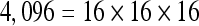
In order to assess how platforms scale when the number of trajectory points in the results increase, the procedure was applied multiple times with a varying number of seed points. For each setup–dataset–platform combination, the density of seed points within the VOI was increased each time the procedure was applied by adding 1 seed to each dimension, so that, for instance, in the first execution, the density was 1 × 1 × 1, for a total of 1 seed point; in the second execution, the density was 2 × 2 × 2, for a total of 8 seed points. The number of seed points, therefore, grows exponentially over time and is given by the function f(x) = x³. The procedure was applied up to a limit of 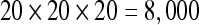seeds. When running experiments, not only the total execution time was recorded, but also the time each iteration of the VOI-sweeping procedure took to be completed and the total number of trajectory points it found.

Figure 3 shows, for all three datasets, the mean number of trajectory points generated by the iterations of the VOI-sweeping procedure. There is no need for a separate graph for each hardware–platform combination because there is very little variation in the actual results generated by them. These differences are a natural product of different floating-point environments, and a broader discussion of the effects of floating-point operations on fiber tracking is given by a previous work.²¹

Fig. 3.

Mean number of trajectory points against number of seed points for all three datasets. The number of seed trajectory points grows linearly with the number of seed points. Here, filled diamond, dataset 1; inverted filled triangle, dataset 2; filled square, dataset 3.

Dataset 1 generates a greater number of trajectory points than datasets 2 and 3 for the same number of seeds, which implies that the fiber trajectories for that dataset are longer. As an example, when fiber tracking is executed with almost 5,000 seeds, the mean number of trajectory points found in dataset 1 is close to 100,000, whereas, in dataset 2, a little more than 60,000 trajectory points were found on average. This simply reflects differences inherent to each dataset, and determining the exact cause (be it the signal-to-noise ratio, the actual brain volume, or some other factor) is beyond the scope of this paper.

The number of trajectory points a fiber tracking algorithm finds is the main factor that influences execution time. Figure 4 contains scatterplots for all hardware–platform combinations, showing, for all three datasets, how much time each one of the iterations of the VOI-sweeping procedure took to complete and the number of trajectory points it found. In all cases, there is a clear linear trend; but for GPUs, the execution time grows more slowly as the number of trajectory points increase, indicating that they achieved a higher performance than that achieved by the CPUs.

Fig. 4.

Scatterplots showing the number of trajectory points and the time taken to process them. Here, filled diamond, dataset 1; inverted filled triangle, dataset 2; filled square, dataset 3.

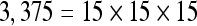
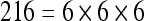
The actual FPS rate achieved by the CPUs and GPUs of both setups is given by the graph in Figure 5. When the number of seeds is very small (less than 30), CPUs perform better than GPUs, because the latter has a fixed minimum cost for the execution of any amount of fiber tracking. For a larger, and therefore more useful, number of seeds, the FPS rate achieved by GPUs is consistently higher. The line that crosses horizontally the graph at 10 FPS indicates the interactivity limit, as established in the section Definition of Real-Time Interactive Fiber Tracking. The highest seed density at which each setup–platform–dataset combination could still keep an interactive FPS rate is given by Table 2. While the CPU could not sustain a mean 10 FPS rate with more than 125 seeds, all GPUs were able to keep that rate with at least 1,728 seeds. In particular, for all three datasets, the GPU of setup 2 was able to maintain the interactive FPS rate with at least 3,375 seeds, which corresponds to a density of 15 × 15 × 15 seeds within the VOI.

Fig. 5.

FPS rate against number of seeds for both setups. Red lines indicate GPU and green lines CPU. a Setup 1. b Setup 2.

Table 2.

Maximum Seed Density at which each Setup and Platform Was Able to Maintain an Interactive Rate

	Setup 1/GPU	Setup 2/GPU	Setup 1/CPU	Setup 2/CPU
Dataset 1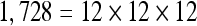
Dataset 2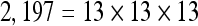
Dataset 3

The results shown by Table 2 imply that, for the hardware configurations used in our experiments, only the GPU was able to fully comply with the definition of real-time interactive fiber tracking given in Definition of Real-Time Interactive Fiber Tracking, since the tool’s default seed density is 10 × 10 × 10, and for no dataset any of the CPUs was able to sustain an interactive rate with that seed density.

The quality of results presented to the user depends heavily on the number of seeds. A low seed density causes the visualization to seem incomplete and conveys less information than a high seed density. This difference in quality can be seen in Figure 6, which shows two results of fiber tracking executed for dataset 3 with a VOI located at the brain stem, one with a density of seeds and the other with a density of 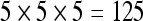seeds, which are the maximum density at which the GPU and the CPU of setup 1, respectively, are able to keep an interactive FPS rate for dataset 3. The results obtained with 3,375 seeds (Fig. 6a) are rich in detail and large in size, while those obtained with 125 seeds (Fig. 6b) are poorer and less meaningful. Thus, while our CPU implementation of fiber tracking could be said to be real-time interactive, it would only be so for a very low number of seeds.

Fig. 6.

Results obtained from dataset 3 with the highest seed density supported by the GPU (a) and the CPU (b) while still being able to sustain an interactive FPS rate. a seeds. b seeds.

The best way to appreciate the interactivity provided by the GPU is by seeing it working. A video showing an interactive real-time fiber tracking exploratory session is available in this article’s electronic supplementary material. The FPS rate in the video is, however, considerably lower than that actually achieved by the application (especially when a large number of trajectory points are being shown) because of limitations in the video capturing tool.

Discussion and Conclusions

In this paper, we have introduced the concept of real-time interactive fiber tracking, which applications can use to provide users with a rich interactive experience, producing a more comfortable and intuitive environment. The main idea behind this concept is that applications should update results immediately after any action taken by the user, however simple it might be. Because real-time interactive fiber tracking depends heavily on the time taken for the application to respond to user actions, we have also defined a method that calculates the FPS rate in an application-independent manner, so that different implementations or even different platforms or subjects can be compared with each other.

We have presented our fiber tracking tool, which implements the concept of real-time interactive fiber tracking. This tool can execute fiber tracking on the GPU or on the CPU, and we have evaluated the performance of both platforms for three datasets. This evaluation has shown that the GPU implementation is able to sustain a rendering rate above 10 FPS for the tool’s default parameters, and the best GPU used in the experiments sustains a rate of 10 FPS for all datasets in a density of 3,375 seed points. Although the hardware setups had a CPU with two cores, only one core was used by the fiber tracking process. However, even if both cores had been used and the performance had been doubled, that setup’s GPU would still have fared better.

Our GPU implementation of fiber tracking was built on top of an extensible multi-purpose prototype workstation, which has been developed by our research group. We adopted the strategy of extending a regular, CPU-oriented radiological workstation with a GPU plug-in that executes a specific procedure, fiber tracking in this case, so that the processing power offered by the computer’s GPU can be fully taken advantage of. We believe that this simple development strategy can be used for other purposes in the context of radiological workstations.

The GPU implementation was evaluated by a neuroradiologist and a radiologist, both users of other fiber tracking tools. The former stated that the fiber tracking tool presented in this paper is faster, more intuitive, and provides a richer interactive experience than the other tools he is acquainted with. The latter stated that our tool not only is faster, but also makes it easier for the fiber tracking results to be manipulated on the screen, which he considers an advantage over the other fiber tracking tools he uses.

The radiologist also remarked that every tool which allows results to be obtained more quickly always impacts the daily medical practice. He summarized his opinion adding that “by making it both faster for images to be obtained and easier for the radiologist to elaborate reports, and by improving the visualization of medical data for physicians, one always causes a positive impact on the daily routine.”

The hardware setups used in our experiments are already outdated, which means that current CPUs and GPUs will achieve an even better performance; in particular, the video cards of both setups, as of early 2009, can be purchased for less than US$100,00.³² The GeForce series, manufactured by NVIDIA,³³ is constantly updated with new video cards, with an ever-increasing floating-point performance. Future experiments with newer GPUs will likely yield a significantly better performance.

GPUs are a promising tool for medical applications in general and fiber tracking in particular. By making it possible to execute existing methods much faster, GPUs provide the user with a more comfortable tool and enables interactivity techniques that previously were not possible with low-cost equipments.

References

- 1.Basser PJ, Mattiello J, Bihan D. MR diffusion tensor spectroscopy and imaging. Biophys J. 1994;66:259–267. doi: 10.1016/S0006-3495(94)80775-1. [DOI] [PMC free article] [PubMed] [Google Scholar]
- 2.Basser PJ, Mattiello J, Bihan D. Estimation of the effective self-diffusion tensor from the NMR spin echo. J Magn Reson B. 1994;103:247–254. doi: 10.1006/jmrb.1994.1037. [DOI] [PubMed] [Google Scholar]
- 3.Bihan D, Mangin JF, Poupon C, Clark CA, Pappata S, Molko N, Chabriat H. Diffusion tensor imaging: concepts and applications. J Magn Reson Imaging. 2001;13:534–546. doi: 10.1002/jmri.1076. [DOI] [PubMed] [Google Scholar]
- 4.Yamada K, Shiga K, Kizu O, Ito H, Akiyama K, Nakagawa M, Nishimura T. Oculomotor nerve palsy evaluated by diffusion-tensor tractography. Neuroradiology. 2006;48:434–437. doi: 10.1007/s00234-006-0070-7. [DOI] [PubMed] [Google Scholar]
- 5.Beaulieu C. The basis of anisotropic water diffusion in the nervous system—a technical review. NMR Biomed. 2002;15:435–455. doi: 10.1002/nbm.782. [DOI] [PubMed] [Google Scholar]
- 6.Conturo TE, Lori NF, Cull TS, Akbudak E, Snyder AZ, Shimony JS, McKinstry RC, Burton H, Raichle ME. Tracking neuronal fiber pathways in the living human brain. Proc Natl Acad Sci USA. 1999;96:10422–10427. doi: 10.1073/pnas.96.18.10422. [DOI] [PMC free article] [PubMed] [Google Scholar]
- 7.Basser PJ, Pajevic S, Pierpaoli C, Aldroubi A. Fiber tract following in the human brain using DT-MRI data. IEICE Trans Inf Syst. 2002;E85-D:15–21. [Google Scholar]
- 8.Hagmann P, Jonasson L, Deffieux T, Meuli R, Thiran J, Wedeen VJ. Fibertract segmentation in position orientation space from high angular resolution diffusion MRI. NeuroImage. 2006;32:665–675. doi: 10.1016/j.neuroimage.2006.02.043. [DOI] [PubMed] [Google Scholar]
- 9.Friman O, Farnebäck G, Westin C. A Bayesian approach for stochastic white matter tractography. IEEE Trans Med Imag. 2006;25:965–978. doi: 10.1109/TMI.2006.877093. [DOI] [PubMed] [Google Scholar]
- 10.Staempfli P, Jaermann T, Crelier GR, Kollias S, Valavanis A, Boesiger P. Resolving fiber crossing using advanced fast marching tractography based on diffusion tensor imaging. NeuroImage. 2006;30:110–120. doi: 10.1016/j.neuroimage.2005.09.027. [DOI] [PubMed] [Google Scholar]
- 11.Mori S, Zijl PCM. Fiber tracking: principles and strategies—a technical review. NMR Biomed. 2002;15:468–480. doi: 10.1002/nbm.781. [DOI] [PubMed] [Google Scholar]
- 12.Dellani PR, Glaser M, Wille PR, Vucurevic G, Stadie A, Bauermann T, Tropine A, Perneczky A, Wangenheim A, Stoeter P. White matter fiber tracking computation based on diffusion tensor imaging for clinical applications. J Digit Imaging. 2007;20:88–97. doi: 10.1007/s10278-006-0773-7. [DOI] [PMC free article] [PubMed] [Google Scholar]
- 13.Pajevic S, Aldroubi A, Basser PJ. A continuous tensor field approximation of discrete DT-MRI data for extracting microstructural and architectural features of tissue. J Magn Reson. 2002;154:85–100. doi: 10.1006/jmre.2001.2452. [DOI] [PubMed] [Google Scholar]
- 14.BrainLAB. iPlan BOLD MRI Mapping. Available at http://www.brainlab.com/. Visited on 18 March 2009.
- 15.Brain Innovation B.V. BrainVoyager QX. Available at http://www.brainvoyager.com/. Visited on 18 March 2009.
- 16.Goebel R, Esposito F, Formisano E. Analysis of functional image analysis contest (FIAC) data with Brainvoyager QX: from single-subject to cortically aligned group general linear model analysis and self-organizing group independent component analysis. Hum Brain Mapp. 2001;27:392–401. doi: 10.1002/hbm.20249. [DOI] [PMC free article] [PubMed] [Google Scholar]
- 17.Roebroeck A, Galuske R, Formisano E, Chiry O, Bratzke H, Ronen I, Kim DS, Goebel R. High-resolution diffusion tensor imaging and tractography of the human optic chiasm at 9.4 T. NeuroImage. 2008;39:157–186. doi: 10.1016/j.neuroimage.2007.08.015. [DOI] [PubMed] [Google Scholar]
- 18.Jeong W, Fletcher P, Tao R, Whitaker R. Interactive visualization of volumetric white matter connectivity in DT-MRI using a parallel-hardware Hamilton–Jacobi solver. IEEE Trans Vis Comput Graph. 2007;13:1480–1487. doi: 10.1109/TVCG.2007.70571. [DOI] [PubMed] [Google Scholar]
- 19.Petrovic V, Fallon J, Kuester F. Visualizing whole-brain DTI tractography with GPU-based tuboids and LoD management. IEEE Trans Vis Comput Graph. 2007;13:1488–1495. doi: 10.1109/TVCG.2007.70532. [DOI] [PubMed] [Google Scholar]
- 20.McGraw T, Nadar M. Stochastic DT-MRI connectivity mapping on the GPU. IEEE Trans Vis Comput Graph. 2007;13:1504–1511. doi: 10.1109/TVCG.2007.70597. [DOI] [PubMed] [Google Scholar]
- 21.Mittmann A, Comunello E, Wangenheim A. Diffusion tensor fiber tracking on graphics processing units. Comput Med Imaging Graph. 2008;32:521–530. doi: 10.1016/j.compmedimag.2008.05.006. [DOI] [PubMed] [Google Scholar]
- 22.Mittmann A, Dantas MAR, von Wangenheim A: Design and Implementation of Brain Fiber Tracking for GPUs and PC Clusters. Proc. 21st International Symposium on Computer Architecture and High Performance Computing SBAC-PAD, São Paulo, 101–108, 2009.
- 23.Köhn A, Klein J, Weiler F, Peitgen H-O: A GPU-based fiber tracking framework using geometry shaders. Proc. of SPIE Medical Imaging, Orlando, 72611J–72611J10, 2009.
- 24.Kwatra A, Prasanna V, Singh M: Accelerating DTI tractography using FPGAs. Proc. 20th International Parallel and Distributed Processing Symposium IPDPS, 1–8, 2006.
- 25.Owens JD, Luebke D, Govindaraju N, Harris M, Krüger J, Lefohn AE, Purcell TJ: A Survey of General-Purpose Computation on Graphics Hardware. Eurographics 2005, State of the Art Reports, 21–51, 2005.
- 26.PC Perspective. NVIDIA Tesla High Performance Computing—GPUs Take a New Life. Available at http://www.pcper.com/article.php?aid=424. Accessed 18 March 2009.
- 27.Buck I: GPU computing with NVIDIA CUDA. ACM SIGGRAPH 2007 courses.
- 28.NVIDIA. NVIDIA website. Available at http://www.nvidia.com/. Accessed 14 November 2008.
- 29.Mark WR, Glanville RS, Akeley K, Kilgard MJ: Cg: a system for programming graphics hardware in a C-like language. Proceedings of the ACM SIGGRAPH conference, San Diego, 896–907, 2003.
- 30.Bammer R, Auer M: Correction of eddy-current induced image warping in diffusion-weighted single-shot EPI using constrained non-rigid mutual information image registration. Proc. 9th ISMRM, Glasgow, 2001.
- 31.Skare S, Anderson JLR: Simultaneous correction of eddy currents and motion in DTI using the residual error of the diffusion tensor: comparisons with mutual information. Proc. 10th ISMRM, Hawaii, 2002.
- 32.Newegg. Available at http://www.newegg.com/. Accessed 18 March 2008.
- 33.NVIDIA. NVIDIA GeForce family. Available at http://www.nvidia.com/object/geforce_family.html. Accessed November 14, 2008.
Associated Data
This section collects any data citations, data availability statements, or supplementary materials included in this article.
Supplementary Materials
Below is the link to the electronic supplementary material.