Parametric Representation of Cortical Surface Folding based on Polynomials

Abstract

The development of folding descriptors as an effective approach for describing geometrical complexity and variation of the human cerebral cortex has been of great interests. This paper presents a parametric representation of cortical surface patches using polynomials, that is, the primitive cortical patch is compactly and effectively described by four parametric coefficients. By this parametric representation, the patterns of cortical patches can be classified by either model-driven approach or data-driven clustering approach. In the model-driven approach, any patch of the cortical surface is classified into one of eight primitive shape patterns including peak, pit, ridge, valley, saddle ridge, saddle valley, flat and inflection, corresponding to eight sub-spaces of the four parameters. The major advantage of this polynomial representation of cortical folding pattern is its compactness and effectiveness, while being rich in shape information. We have applied this parametric representation for segmentation of cortical surface and promising results are obtained.

1 Introduction

Quantitative description of the geometrical complexity and variability of the human cerebral cortex has been of great interests. The development of shape descriptors that model the cortical folding pattern is essential to understand brain structure and function. Recent study has shown that cortical folding pattern could be used to predict brain function [1]. Besides, quantitative cortical folding descriptor may help reveal the underlying mechanism of cortical gyrification [2, 3] and provide clues for the understanding of abnormal cortical folding in brain disorders [4, 5].

In order to quantitatively and effectively measure cortical folding, a couple of attempts have been made in literature. In [6], the cortical surface area was compared to its external surface areas to determine the degree of folding. In [7], the gyrification index (GI) was proposed to compute the ratio between the pial contour and the outer contour in successive coronal sections, which has been widely used in many studies [8, 9]. Recently, the GI measurement was extended to 3D [10]. Curvature, which is a 3D parametric measurement, was also widely used as a metric to study cortical folding pattern [11]. These descriptors have their own advantages, but also have their limitations. Novel folding pattern descriptors that incorporate 3D geometric shape pattern information are still to be developed.

In this paper, a compact parametric model with four polynomial coefficients is developed to describe cortical surface patch shape pattern. By this parametric representation, the patterns of cortical patches can be classified by either model-driven or data-driven clustering approaches. In particular, by taking the advantage of symmetry of cortical patch, the model-driven approach is able to classify the patches into one of the eight primitive shape patterns: peak, pit, ridge, valley, saddle ridge, saddle valley, flat and inflection, which altogether cover the 4-dimensional parametric space. In order to show the effectiveness of this method, we have applied this parametric representation for segmentation of cortical surfaces of 80 subjects, and promising results are obtained.

2 Methods

2.1 Parametric Polynomial Model

Our work is inspired by the 2D power function based representation of tectonic folding presented in [12]. Our parametric polynomial surface model is represented as:

$$z={\displaystyle \sum _{i=1}^m{a}_i{x}^i+{\displaystyle \sum _{j=1}^n{b}_j{y}^j}}$$ (1)

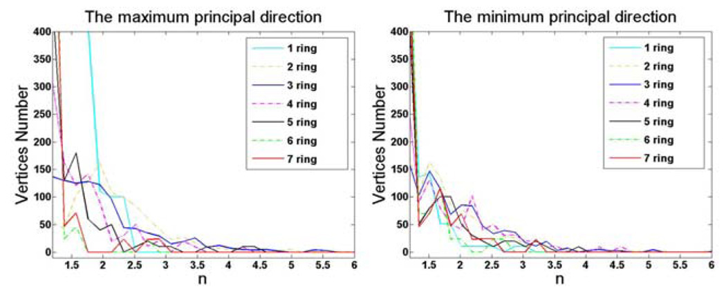
where x, y and z are vertex coordinates, a_i and b_j are coefficients. In order to decide the maximal values of m and n, we fitted the 2D power function to 1000 randomly selected patches along two directions corresponding to two principal curvatures of the central vertex of each patch. The sizes of surface patch are ranging from 1-ring to 7-ring neighborhood. The statistical results of the exponent n are shown in Fig. 1. It is evident that the exponent n is rarely over 3. We have similar results for the exponent m.

Fig. 1.

The statistical distribution of exponent n in power function fitting.

Therefore, we present the cortical surface patches by polynomials in the following format:

$$Z=a{X}^2+b{Y}^2+c{X}^3+d{Y}^3$$ (2)

where a and b describe the mirror symmetric components of the patch, while c and d represent the rotational symmetric components.

2.2 Model Fitting

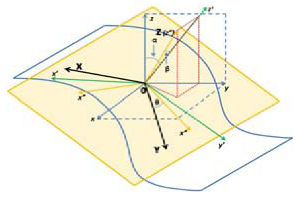
We use the Frenet frame as the coordinate system to estimate parameters in Eq. (2). The origin of Frenet frame coincides with the central vertex of the patch, and the central vertex’s normal is regarded as the Z-axis of the frame that always points towards outside of the brain. The X-axis and Y-axis are set free in the beginning, and will be determined later by the estimated parameters. So the Frenet frame is called semi-free Frenet frame here (Fig. 2). Eq. (2) is rewritten as f(θ⃗, x⃗) = 0, and we have:

$$f(\overrightarrow{\theta },\overrightarrow{x})=a{X}^2+b{Y}^2+c{X}^3+d{Y}^3-Z$$ (3)

where θ⃗ = (a, b, c, d)^T, and x⃗ = (X, Y, Z)^T. It is worth noting that (X, Y, Z)^T is the coordinates in the semi-free Frenet frame. Therefore, all the coordinates of surrounding patch vertices should be rotated as follow:

$$\left[\begin{array}{c}\hfill X\hfill \\ \hfill Y\hfill \\ \hfill Z\hfill \end{array}\right]=\left[\begin{array}{ccc}\hfill 1\hfill & \hfill 0\hfill & \hfill 0\hfill \\ \hfill 0\hfill & \hfill \text{cos}\alpha \hfill & \hfill -\text{sin}\alpha \hfill \\ \hfill 0\hfill & \hfill \text{sin}\alpha \hfill & \hfill \text{cos}\alpha \hfill \end{array}\right]\left[\begin{array}{ccc}\hfill \text{cos}\beta \hfill & \hfill 0\hfill & \hfill -\text{sin}\beta \hfill \\ \hfill 0\hfill & \hfill 1\hfill & \hfill 0\hfill \\ \hfill \text{sin}\beta \hfill & \hfill 0\hfill & \hfill \text{cos}\beta \hfill \end{array}\right]\left[\begin{array}{ccc}\hfill \text{cos}\theta \hfill & \hfill -\text{sin}\theta \hfill & \hfill 0\hfill \\ \hfill \text{sin}\theta \hfill & \hfill \text{cos}\theta \hfill & \hfill 0\hfill \\ \hfill 0\hfill & \hfill 0\hfill & \hfill 1\hfill \end{array}\right](\left[\begin{array}{c}\hfill x_i\hfill \\ \hfill y_i\hfill \\ \hfill z_i\hfill \end{array}\right]-\left[\begin{array}{c}\hfill x_0\hfill \\ \hfill y_0\hfill \\ \hfill z_0\hfill \end{array}\right])$$ (4)

where [x₀, y₀, z₀]^T the coordinate of the central vertex; α and β are two angles between the axes of different coordinates frames; θ is a new parameter introduced to rotate the semi-free Frenet frame on X-Y plane. Then, the Eq. (3) is rewritten as:

$$f(\overrightarrow{u},\overrightarrow{x})=0$$ (5)

where parameter u⃗ = (a, b, c, d, θ)^T, and x⃗ = (x_i, y_i, z_i)^T.

Fig. 2.

The semi-free Frenet frame.

To estimate the parameters in Eq. (5), the non-linear least square fitting (NLLSF) method is adopted to fit the patch. There is no closed-form solution to a non-linear least squares problem. However, the nonlinear problem can be iteratively linearized and becomes a linear least squares problem in each iteration. In order to apply the NLLSF method to our model, Eq. (5) is rewritten in the following way:

$$z=\tilde{f}(\overrightarrow{u},\overrightarrow{x})$$ (6)

Supposing there are n vertices on the patch, the model fitting algorithm is as follows:

• Step.1. Initialize parameter u⃗⁰, maximum iteration times N and ε, k = 0;

• Step.2. Compute the shift vector Δu⃗^k by equations written in matrix notation as

  $$\mathrm{\Delta }{\overrightarrow{u}}^k={(J^{T}J)}^{-1}{J}^T\mathrm{\Delta }\overrightarrow{z}$$ (7)

  where Δz⃗ = (z₁ − f̃(u⃗^k, x⃗₁),⋯z_n − f̃(u⃗^k, x⃗_n))^T, and J is the Jacobian matrix.

• Step.3. If ‖Δu⃗^k‖ ≤ ε, or k > N, stop iteration and output u⃗^k; else go to Step.4;

• Step.4. u⃗^k+1 = u⃗^k + Δu⃗^k, k = k + 1, go to Step.2.

A critical issue in the polynomial model fitting is the patch size. Generally, the larger the patch is, the more shape information it will enclose. However, if the patch is too large, its folding shape will be too asymmetric to be described by polynomials. Both qualitative and quantitative experiments show that 3-ring neighborhood is good to maintain the symmetry property of surface patches.

2.3 Model Pattern Classification

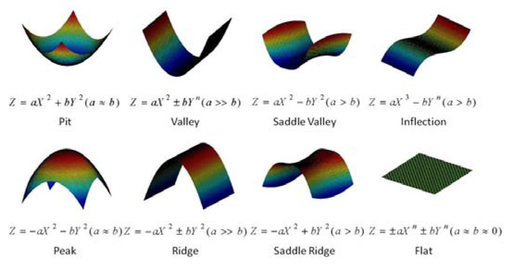
As mentioned above, the estimated parameter sets (a, b, c, d)^T will be used to determine the X- and Y- axis as follows. Intuitively, the largest value in a, b, c and d will dominate the shape of a surface patch, as shown in Fig. 3. For example, in the valley shape, the parameter a will be the largest and dominate the patch shape. So for the sake of convenience, we use the X-axis to represent the dominating direction, i.e., the largest absolute value is either a or c, and Y-axis is orthogonal to X-axis. If b or d is of the largest absolute value, we switch a and c with b and d.

Fig. 3.

Eight primitive folding patterns of surface patches.

2.3.1 Model-driven Method

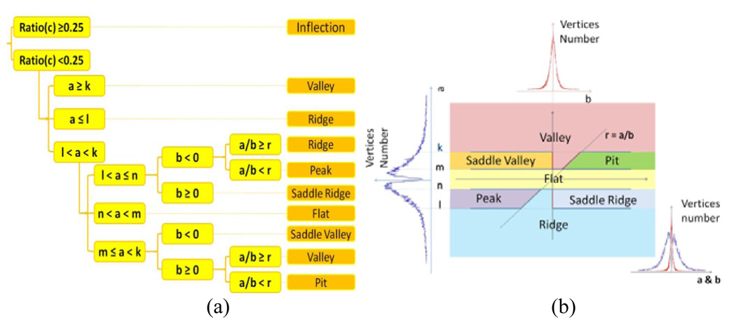
The surface patch patterns represented by above polynomial model are classified into eight primitive fold patterns including peak, pit, ridge, valley, saddle ridge, saddle valley, flat, and inflection as shown in Fig. 3. This classification approach is similar to that in [14]. The decision tree for this model-based classification method is shown in Fig. 4, where the absolute component ratio is defined as:

$$\text{Ratio}(\lambda )=\frac{\left|\lambda \right|}{\left|a\right|+\left|b\right|+\left|c\right|+\left|d\right|},\lambda \in (a,b,c,d)$$ (8)

Fig. 4.

(a) The clustering decision tree. (b) The parametric subspaces of a and b for different patterns.

This classification method (Fig. 4a) covers the entire four dimensional space of parameter a, b, c and d. The parameter c or d will determines the inflection pattern if any of them is larger than 0.25. Otherwise, the parameter a and b will decide the other shape patterns as shown in Fig. 4b. Currently, all of these thresholds are determined by expert visual inspections.

2.3.2 Data-driven Method

We applied the K-means clustering method to classify the surface patches represented by the four coefficients into different patterns. The distance measurement between patches is simply the summed squared Euclidean distance of the four model parameters.

3 Results

The proposed method is applied on 80 randomly selected normal brains in the OASIS MR image database. All the topologically correct and geometrically accurate cortical surfaces are generated via the method in [15].

3.1 Results of Model-driven Method

The model-driven folding pattern classification method introduced in Section 2.3.1 was applied to 80 cortical surfaces. As an example, Fig. 5 shows the primitive patch shape classification result on a cortical surface. Currently, the thresholds k, l, n, m in Fig. 4a used in this classification are manually determined. Fig. 5 clearly illustrates the distributions of the eight primitive folding patterns over the cortex. Ridges and valleys are commonly distributed on the crests of gyri and at the bottoms of sulci. Pits mostly sit in bowl-shaped sulcal regions. Peaks are more likely to be the joints of connected gyri. Inflections tend to be slender lines separating straight and long slopes where gyral regions meet the sulcal regions. The flats are located on smooth walls beneath the crests of gyri or the plain-shaped gyri crests. Saddle ridges and saddle valleys are distributed relatively evenly. The result in Fig. 5 shows that the proposed cortical patch representation and classification method can properly discriminate the shape differences across the whole cortical surface. Our preliminary results show that the percentage of flats is significantly higher in normal brains than Autism patients.

Fig. 5.

The model-driven classification result on a cortical surface. Eight primitive folding patterns are represented by different colors. The blue dots on the right patches represent the central vertices of the corresponding patches.

In order to evaluate the accuracy of the folding pattern classification methods, 600 patches randomly selected from 80 cortical surfaces are manually classified into the 8 patterns in Fig. 5 respectively. The automatic classification results are compared with the manual labeling results, and Table 1 summarizes the sensitivity and specificity of the automatic classification method. It is apparent that the automatic folding pattern classification method is quite accurate, given the high sensitivity and specificity over 0.9.

Table 1.

The comparison result for model-driven method.

Cluster name	Saddle Valley	Inflection	Saddle Ridge	Ridge	Flat	Peak	Pit	Valley
sensitivity	0.8333	0.9091	0.8636	0.9792	0.8438	0.9483	0.8710	0.9792
specificity	0.9929	0.9827	1	0.9762	0.9873	0.9752	0.9926	0.9921

3.2 Results of Data-driven Method

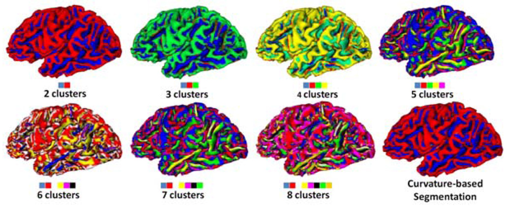
Fig. 6 shows the data-driven classification results with the number of clusters ranging from 2 to 8. With the increase of cluster numbers, more detailed shape patterns are generated. Especially, the 2-classes clustering results, parcelling cortex into gyral and sulcal regions, is similar to the curvature based parcellation of cortex [13] as shown in the right bottom of Fig. 6. Also, to evaluate the accuracy of the methods, the same 600 surface patches are manually classified into 5 clusters respectively. The data-driven automatic clustering results are compared with the manual labeling, and the results are provided in Table 2. Evidently, the sensitivity and specificity of the data-driven clustering method are quite high.

Fig. 6.

K-means clustering results with the number of clusters ranging from 2 and 8.

Table 2.

The comparison result for data-driven method.

Cluster index	Cluster 1	Cluster 2	Cluster 3	Cluster 4	Cluster 5
sensitivity	0.9833	0.9661	0.9672	0.9333	0.9000
specificity	0.9958	0.9917	0.9916	0.9833	0.9750

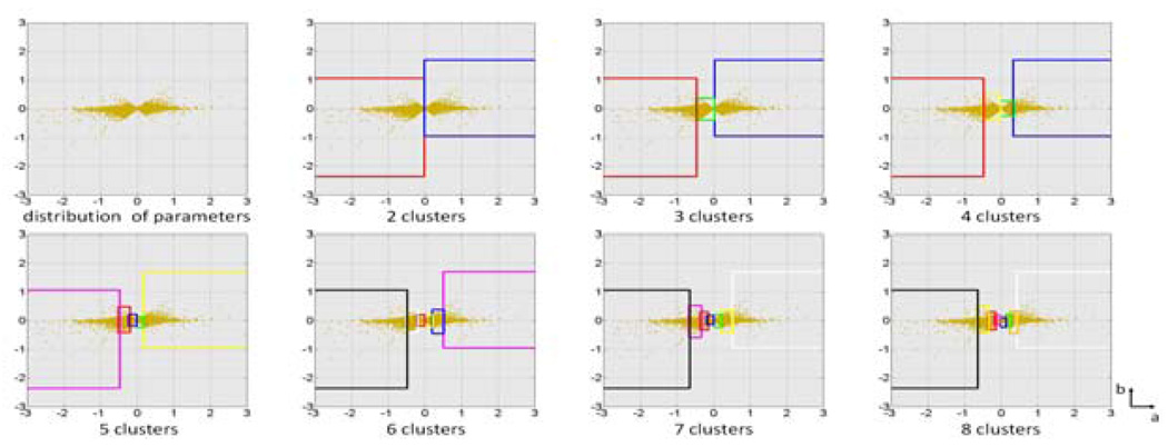
To investigate the parameter distribution in the data-driven clustering, we take an arbitrary case with 47600 vertices as an example. Distributions of a and b, the two dominant parameter (see Table 3), in each clustering result using different cluster numbers from 2 to 8 are shown in Fig. 7.

Table 3.

The numbers of dominant parameters.

Dominant parameter	a	b	c	d
Number of vertices	47258	11244	1802	472

Fig. 7.

Distribution of parameter a and b for each cluster across different cluster numbers. The boxes are color coded according to the corresponding clusters in Fig. 6.

4 Discussion and Conclusion

Compared to previous cortical folding descriptors such as curvature and gyrification index, the proposed polynomial parametric representation is able to differentiate cortical surface patches into primitive shape patterns. The major advantage of the polynomial representation of cortical folding pattern is its compactness and effectiveness, while being rich in shape information. However, the polynomial representation in Eq. (2) is not perfect. It requires that the shape of the patch in consideration to be symmetric. As the size of surface patch grows, e.g., larger than 4-ring or 5-ring neighborhood, the symmetry requirement might be violated. Also, the shape complexity of the cortical patch might be beyond the description ability of the polynomial model in Eq. (2). In the future, more factors such as twisting effect should be added into the shape model in Eq. (2) for better description capability of cortical shape patterns. The work presented in this paper demonstrates that parametric shape descriptor is a powerful tool to model cortical folding patterns. Potential applications include automatic parcellation of cortical surface as shown in Fig. 5 and Fig. 6, automatic recognition of cortical structures using folding patterns as features, as well as studies of abnormal folding patterns in brain diseases.

References

- 1.Fischl B, Rajendran N, Busa E, Augustinack J, Hinds O, Yeo BT, Mohlberg H, Amunts K, Zilles K. Cortical Folding Patterns and Predicting Cytoarchitecture. Cereb Cortex. 2008;18(8):1973–1980. doi: 10.1093/cercor/bhm225. [DOI] [PMC free article] [PubMed] [Google Scholar]
- 2.Van Essen DC. A tension-based theory of morphogenesis and compact wiring in the central nervous system. Nature. 1997;385:313–318. doi: 10.1038/385313a0. [DOI] [PubMed] [Google Scholar]
- 3.Toro R, Burnod Y. A Morphogenetic Model of the Development of Cortical Convolutions. Cerebral Cortex. 2005;15:1900–1913. doi: 10.1093/cercor/bhi068. [DOI] [PubMed] [Google Scholar]
- 4.Van Essen DC, Dierker D, Snyder AZ, Raichle ME, Reiss AL, Korenberg J. Symmetry of Cortical Folding Abnormalities in Williams Syndrome Revealed by Surface-Based Analyses. J. Neurosci. 2006;26(20):5470–5483. doi: 10.1523/JNEUROSCI.4154-05.2006. [DOI] [PMC free article] [PubMed] [Google Scholar]
- 5.Sallet PC, Elkis H, Alves TM, Oliveira JR, Sassi E, Campi de Castro C, Busatto GF, Gattaz WF. Reduced Cortical Folding in Schizophrenia: An MRI Morphometric Study. Am J Psychiatry. 2003;160:1606–1613. doi: 10.1176/appi.ajp.160.9.1606. [DOI] [PubMed] [Google Scholar]
- 6.Elias H, Schwartz D. Surface areas of the cerebral cortex of mammals determined by stereological methods. Science. 1969;166:111–113. doi: 10.1126/science.166.3901.111. [DOI] [PubMed] [Google Scholar]
- 7.Zilles K, Armstrong E, Schleicher A, Kretschmann HJ. The human pattern of gyrification in the cerebral cortex. Anat Embryol (Berl) 1988;179:173–179. doi: 10.1007/BF00304699. [DOI] [PubMed] [Google Scholar]
- 8.Hardan AY, Jou RJ, Keshavan MS, Varma R, Minshew NJ. Increased frontal cortical folding in autism: a preliminary MRI study. Psychiatry Research. 2004;131(3):263–268. doi: 10.1016/j.pscychresns.2004.06.001. [DOI] [PubMed] [Google Scholar]
- 9.Neal J, Takahashi M, Silva M, Tiao G, Walsh CA, Sheen VL. Insights into the gyrification of developing ferret brain by magnetic resonance imaging. J Anat. 2007;210(1):66–77. doi: 10.1111/j.1469-7580.2006.00674.x. [DOI] [PMC free article] [PubMed] [Google Scholar]
- 10.Schaer M, Cuadra MB, Tamarit L, Lazeyras F, Eliez S, Thiran JP. A Surface-based approach to Quantify Local Cortical Gyrification. IEEE Trans. TMI. 2008;27(2):161–170. doi: 10.1109/TMI.2007.903576. [DOI] [PubMed] [Google Scholar]
- 11.Cachia A, Mangin JF, Rivière D, Kherif F, Boddaert N, Andrade A, Papadopoulos-Orfanos D, Poline JB, Bloch I, Zilbovicius M, Sonigo P, Brunelle F, Régis J. A Primal Sketch of the Cortex Mean Curvature:a Morphogenesis Based Approach to Study the Variability of the Folding Patterns. IEEE Trans. TMI. 2003;22(6):754–765. doi: 10.1109/TMI.2003.814781. [DOI] [PubMed] [Google Scholar]
- 12.Lisle RJ, Fernández Martínez JL, Bobillo-Ares N, Menéndez O, Aller J, Bastida F. FOLD PROFILER: A MATLAB—based program for fold shape classification. Computers & Geosciences. 2006;32:102–108. [Google Scholar]
- 13.Li G, Guo L, Nie J, Liu T. Automatic cortical sulcal parcellation based on surface principal direction flow field tracking. NeuroImage. 2009;46(4):923–937. doi: 10.1016/j.neuroimage.2009.03.039. [DOI] [PMC free article] [PubMed] [Google Scholar]
- 14.Besl PJ, Jain RC. Segmentation Through Variable-Order Surface Fitting. IEEE Trans. PAMI. 1988;10(2):167–192. [Google Scholar]
- 15.Liu T, Nie J, Tarokh A, Guo L, Wong ST. Reconstruction of central cortical surface from brain MRI images: method and application. Neuroimage. 2007;40(3):991–1002. doi: 10.1016/j.neuroimage.2007.12.027. [DOI] [PMC free article] [PubMed] [Google Scholar]