Abstract
We present a novel integrated wavelet-domain based framework (w-ICA) for 3-D de-noising functional magnetic resonance imaging (fMRI) data followed by source separation analysis using independent component analysis (ICA) in the wavelet domain. We propose the idea of a 3-D wavelet-based multi-directional de-noising scheme where each volume in a 4-D fMRI data set is sub-sampled using the axial, sagittal and coronal geometries to obtain three different slice-by-slice representations of the same data. The filtered intensity value of an arbitrary voxel is computed as an expected value of the de-noised wavelet coefficients corresponding to the three viewing geometries for each sub-band. This results in a robust set of de-noised wavelet coefficients for each voxel. Given the decorrelated nature of these de-noised wavelet coefficients; it is possible to obtain more accurate source estimates using ICA in the wavelet domain. The contributions of this work can be realized as two modules. First, the analysis module where we combine a new 3-D wavelet denoising approach with better signal separation properties of ICA in the wavelet domain, to yield an activation component that corresponds closely to the true underlying signal and is maximally independent with respect to other components. Second, we propose and describe two novel shape metrics for post-ICA comparisons between activation regions obtained through different frameworks. We verified our method using simulated as well as real fMRI data and compared our results against the conventional scheme (Gaussian smoothing + spatial ICA: s-ICA). The results show significant improvements based on two important features: (1) preservation of shape of the activation region (shape metrics) and (2) receiver operating characteristic (ROC) curves. It was observed that the proposed framework was able to preserve the actual activation shape in a consistent manner even for very high noise levels in addition to significant reduction in false positives voxels.
Keywords: functional MRI, 3-D wavelets, denoising, ICA, validation metrics
1. INTRODUCTION
The interest in uncovering functional connections in the brain has grown rapidly with advancements being made in fMRI analysis methodologies, consequently necessitating the exploration of approaches to enhance the pre-processing methods. Researchers in the field of functional neuroimaging have faced a long standing problem in pre-processing fMRI data. Denoising is a common pre-processing step that is applied before analyzing the fMRI data. The most commonly utilized method for this task is to smooth the fMRI image with volumetric Gaussian kernels (Poline et al., 1997). This method is widely applied as it suppresses high-frequency noise and is simple to implement. A drawback of this method is that Gaussian smoothing considerably changes the true intensity values as a function of the size of the smoothing kernel. In addition, the Gaussian smoothing approach suppresses the edge details and other medium-frequency information present in the original image.
Wavelets have been previously applied for de-noising in many medical imaging applications (Bao and Zhang, 2003; Bullmore et al., 2001; Hilton et al., 1996; Unser and Aldroubi, 1996; Xu et al., 1994). The most general procedure is: (i) compute the discrete wavelet transform (DWT) (Mallat, 1999); (ii) utilize an appropriate method to remove or shrink the noisy wavelet coefficients; (iii) reconstruct the image by using an inverse wavelet transform from the de-noised wavelet coefficients. This procedure is usually applied on all the high-frequency wavelet sub-bands obtained post-DWT. A commonly used methodology for de-noising wavelet coefficients as mentioned in (ii) is known as soft thresholding, originally proposed by (Donoho, 1995; Donoho and Johnstone, 1994). A comprehensive comparative study presented by (Wink and Roerdink, 2004) highlighted the differences between various threshold-selection schemes in the WaveLab package (Buckheit et al., 1995) and the commonly used Gaussian smoothing.
Previously, researchers have attempted to apply denoising schemes other than Gaussian smoothing or wavelet-based denoising to fMRI data. Some of the alternate methods include spectral subtraction (Kadah, 2004), spatially adaptive Gaussian smoothing (Tabelow et al., 2006), a novel non-local means filtering approach (He and Greenshields, 2009), and a more recently proposed anisotropic spatial averaging technique (Monir and Siyal, 2009). All of the above methodologies emphasize on denoising fMRI data for further analysis in the spatial domain. There has been little work done in the past involving combinations of 3-D denoising, wavelet transforms and ICA applied in the transform domain for analysis of fMRI data. The w-ICA framework proposed in this paper focuses on applying a source separation approach such as ICA on a decorrelated set of wavelet coefficients obtained through a 3-D wavelet-based denoising scheme applied on each voxel in each sub-band as compared to the above 2-D methods.
The primary motivation behind using Gaussian smoothing kernels is to increase the overall signal-to-noise ratio (SNR). An undesirable effect of this method is that the noise and signal are smoothed together, making it more difficult to accurately separate signal and noise during the later stages of analysis. The results in (Donoho and Johnstone, 1994) show that methods which introduce a high degree of smoothing also tend to produce more false positives, whereas, most wavelet-based methods with lower smoothing properties preserve the shape but may result in a higher number of false negatives.
The ultimate goal of fMRI data analysis is to separate signal components due to true activations from components due to physiological fluctuations and random noise. To achieve this objective, suitable statistical methods are applied to these denoised volumes. Amongst the initially proposed methods, a very popular software package is SPM (Frackowiak, 2004; Friston et al., 1994). SPM is implemented using MATLAB®, and is based on a parametric hypothesis-driven technique. SPM uses a linear model to derive a parameter map from Gaussian smoothed fMRI data (Poline et al., 1997). A relatively new framework that integrates wavelet-based processing with statistical testing (SPM), known as the Wavelet-SPM or WSPM was introduced by (Van De Ville et al., 2006; Van De Ville et al., 2007). This method uses the favorable properties of wavelets, such as decorrelated wavelet coefficients, to adaptively denoise the parameter map (Van De Ville et al., 2006) and perform statistical testing in the spatial domain after reconstruction (Van De Ville et al., 2007). The final detected parameter map in (Van De Ville et al., 2007) is observed to be more closely related to the measured data and has reduced spatial bias as compared to the Gaussian smoothing approach implemented in SPM.
Apart from highly successful parametric methods stated above, wavelet processing has been utilized alongside non-parametric processing techniques. (Long et al., 2004) directly derive well-defined activation maps using a spatially constrained maximum-likelihood criterion on multi-scale representations of the data. (Breakspear et al., 2004) utilized bootstrapping methods in the spatial and spatio-temporal domain. They applied non-parametric null-hypothesis testing on spatiotemporally resampled data in the wavelet domain. This helped preserve spatial and temporal correlations between slices and also maintained the irregular geometry of intracranial images.
A data-driven approach based upon source separation, which is widely used for both task and resting-state data is independent component analysis (ICA) combined with the basic preprocessing steps such as PCA and whitening (Calhoun et al., 2009b; McKeown et al., 1998). This approach identifies components which are maximally independent and linearly mixed; hence each component reflects brain regions which exhibit temporal coherence (functional connectivity). This methodology has been used for a number of biomedical applications in which data can be modeled as a mixture. ICA has also been utilized by researchers to identify signal components with an acceptable level of accuracy for event-related fMRI data (Calhoun et al., 2003). The foremost advantage of ICA is its applicability to detect cognitive patterns for which an a priori temporal model is unavailable. ICA has proven to help reveal inter-subject and inter-event differences in temporal dynamics as well as detect changes with respect to spatially distributed brain networks (Calhoun et al., 2009b). By far the most common application of ICA is extraction of spatially independent brain regions (spatial ICA) although temporal ICA is also possible (Calhoun et al., 2001).
The advantages of wavelet-based processing combined with a source separation technique such as ICA remain unexplored and have not yet been reported with sufficient corroborating and convincing results. Previously, there have been a few attempts to combine the power of wavelet processing (in order to decorrelate data), with a widely applied fMRI analysis technique such as ICA (Azzerboni et al., 2004; Azzerboni et al., 2005; Boroomand et al., 2007; Johnson et al., 2007). A more recent technique that utilizes a combination of wavelet-domain ICA with Wiener filtering of wavelet coefficients is introduced in (Boroomand et al., 2007). They utilize a hybrid approach in order to remove effects of noise on accurate separation of data using ICA. A comparison between Fast ICA and Information maximization ICA is presented followed by the description of a hybrid methodology for denoising manually selected wavelet details. Comparison between different ICA algorithms is performed for data sets with SNR ranging up to 70 dB. At realistic SNR levels (~ 15 – 35 dB), the algorithm performs with a low percent sensitivity (true positive rate) of about 70% with little emphasis on preservation of shape of the activation regions. It may be intuitive to say that the application of Wiener filter in wavelet domain improves the performance of time-domain Wiener filtering, introducing least amount of temporal smoothing, eventually resulting in a good estimate of noise in a least squares sense. (Boroomand et al., 2007; Xu et al., 1994) did not report the false discovery rate (FDR) that is expected to be high due to the aforementioned low-smoothing characteristics of proposed wavelet-wiener filter, and neither compared their results for varying noise frames against other denoising methods such as Wiener filtering on observation data in the spatial domain.
In this paper, we propose a hybrid wavelet-domain ICA framework (w-ICA) for analysis of fMRI data and two novel shape metrics for performance evaluation and measuring shape distortions of the spatial activation regions. Our method is intended to produce minimal loss of details and to minimize large scale intensity variations in the final statistical map as compared to results of conventionally used Gaussian-smoothing based methods. Our proposed methodology utilizes a 3-D stationary discrete wavelet transform for volumetric de-noising and effectively integrates the data-driven ICA approach. The multi-directional nature of the denoising module utilizes the theory that the amount of signal and noise present in a voxel are highly dependent on the signal and noise in its neighboring voxels. Three different de-noised estimates for axial, coronal and sagittal viewing geometries are averaged to compute the final denoised data set. The input to the ICA module is in the transform domain (denoised wavelet coefficients). The algorithm was first tested on hybrid data generated using an additive signal/noise model (see Section 2.1). A comparative analysis is performed between the (i) proposed framework (wavelet denoising + wavelet-domain ICA) and (ii) the conventional framework (Gaussian smoothing + spatial ICA) on the basis of (1) shape preservation and (2) sensitivity-FDR curves (ROC). Hybrid data was generated using a resting state fMRI data set as the baseline signal and a task-related box-car type model as the activation signal. Two different regions of the brain were used as the areas of activation or regions of interest (ROI) – (1) left occipital lobe – visuomotor and (2) left temporal lobe. In addition to above, the proposed framework was applied to real fMRI data set acquired from a single subject performing a simple motor tapping task.
An important advantage of the wavelet transforms especially in context of functional brain imaging is preservation of the shape of activation regions, that is, degree of similarity between the true area of activation before and after denoising. In order to evaluate the efficacy of our proposed framework compared to conventionally used methods, we present two shape descriptors based on morphological measurements of spatial maps corresponding to the activation component.
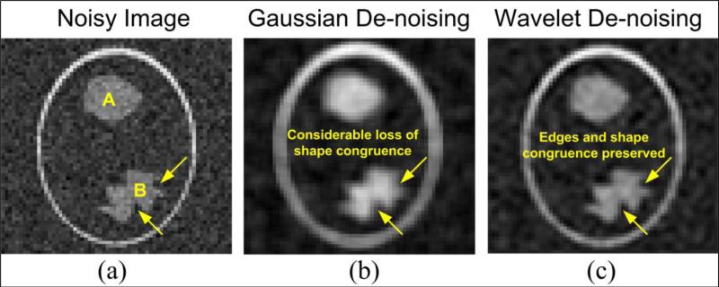
In functional brain imaging, the underlying shape of an activation region (spatial) determined from statistical analysis is an important characteristic which should be preserved. Gaussian smoothing sacrifices the shape of the activated regions in order to bring out the underlying spatial ROI related to the BOLD activation. As such it distorts the original shape resulting in more false positives and loss of edge information. In order to demonstrate this behavior, we performed an experiment as presented in Appendix A. The preservation of shape congruence in case of wavelet-based denoising scheme is expected to serve as a noteworthy advantage in terms of preserving the true area/spread of activations in both multiple subject group data. Thus, such a method is expected to aid in determination of bio-markers for brain disorders such as schizophrenia.
The remainder of this paper is organized as follows: we first present a detailed description of the proposed algorithm in Section 2 accompanied by description of various performance measures applied for evaluation of results. Results are presented in Section 3 and conclusions are drawn in Section 4.
2. PROPOSED ALGORITHM & VALIDATION
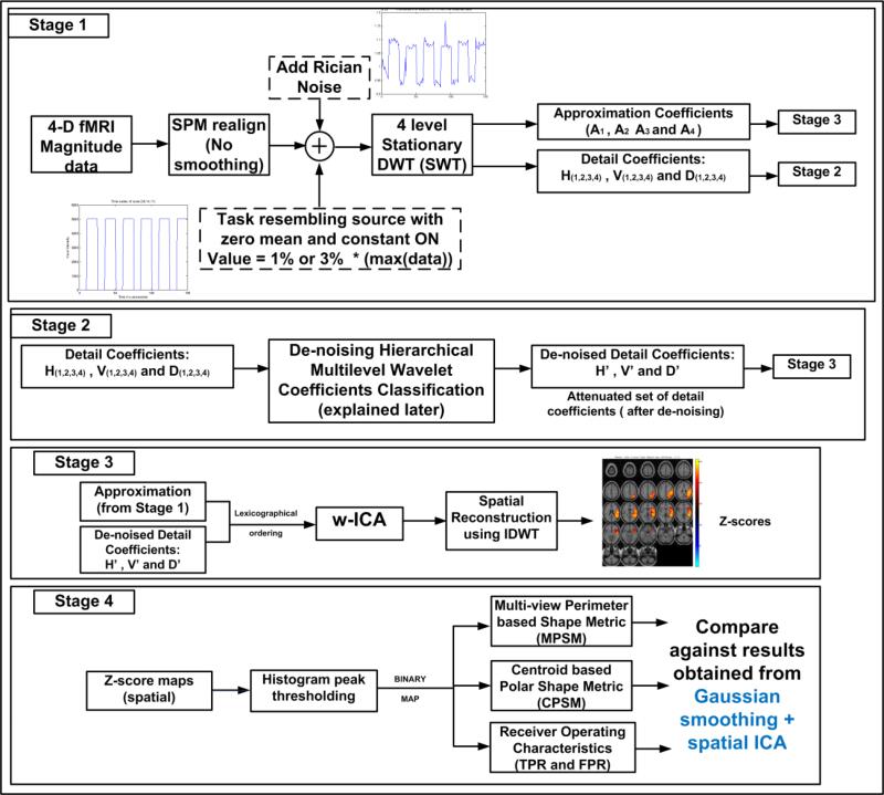
To demonstrate the working and validation of our proposed method, we utilize four stages that describe the most important steps known as: (1) Generation of hybrid data and estimation of wavelet coefficients or data generation and wavelet transform (DGWT); (2) proposed denoising methodology or hierarchical and multi-directional coefficient shrinkage (HMCS); (3) ICA on denoised wavelet coefficients (w-ICA) and wavelet reconstruction; and lastly (4) performance evaluation using ROC statistics in addition to two novel shape metrics proposed in this paper: (a) multi-view perimeter based shape metric (MPSM) and (b) centroid based polar shape metric (CPSM). The underlying reasons for including Stage 4 are to corroborate the benefits of our proposed wavelet based methodology and provide a foundation to researchers for performing quality tests on several available algorithms for fMRI data analysis. At the end of this section, the reader will be able to quantify and compare the advantages of the w-ICA framework over the conventionally used denoising and signal separation methods for fMRI data. A high level block diagram of the proposed algorithm and the four constituting stages is shown in Fig. 1. Output of each stage is shown as the input to the next respective stage.
Figure 1. A high level block diagram of the proposed framework.
Stage 1 includes data generation and wavelet transforms (DGWT), Stages 2 & 3 show the working of the proposed w-ICA framework (HMCS + w-ICA) followed by application of performance evaluation metrics (MPSM/CPSM) in Stage 4.
2.1 Data Generation and Wavelet Transform: DGWT
In this section we present the details related to the generation and design of the data sets used for testing of the proposed framework in addition to some technical concepts involving discrete wavelet transforms (DWT) and their application for this work.
2.1.1 Data Generation – Software Phantoms
For this study, the artificial data was generated using a real resting state fMRI data set as the baseline signal and by adding activations of varying percent signal change. The data was primarily divided on the basis of known anatomical regions of the brain. The spatial maps corresponding to the regions of interest (ROI) were created by utilizing the software package WFU Pick Atlas (Lancaster et al., 2000) . The left temporal lobe and the left occipital lobe regions were selected as the two main ROIs on the basis of number of voxels and their complex shape. In order to demonstrate the key advantages of our proposed algorithm over conventional smoothing methods, we took into account two primary features – complex shape and large number of voxels while selecting these two anatomical regions. These data sets are referred to as „software phantoms’ in the remaining portion of this paper.
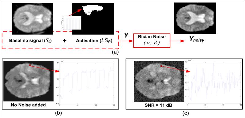
In our simulations, there are three main aspects associated with the generation of the fMRI data set: (1) baseline signal (no task-related activation); (2) signal level of activation voxels; (3) noise level in data set. For activation signal, a simple block design type signal was used (six blocks of ten-second off time, fifteen second on time) lasting 150 seconds. 4-D binary masks corresponding to each region of interest (temporal lobe, occipital lobe) were multiplied by this activation signal in order to simulate a data set closely corresponding to BOLD related activity. The question here to be asked is how much intensity change is a fair representative of the change in BOLD signal when a task-related activity occurs in the brain. For our simulations, we generate data sets for two signal levels – 1% and 3%, of the maximum numerical value in resting state fMRI data used as the baseline signal. These values were chosen based on the fact that task-related BOLD signal change is very small compared to the total spatial and temporal variability across images (Huettel et al., 2004). The block diagram shown in Fig. 2 depicts the process applied for the generation of a software phantom.
Figure 2. Software phantom data generation.
(a) Illustration of phantom data generation: a single slice depicting baseline intensity values along with the block design type task related time course and the ROI mask (temporal lobe). These are added together and input to the Rician noise model to obtain the noisy slice (Ynoisy); the bottom two figures depict the time course and intensity representations when (b) no noise is added, and when (c) there is added Rician noise.
As additional noise, Rician distributed noise is introduced in to the data set after the superposition of the 4-D activation mask as explained above. Eqns. (1) and (2) summarize the data generation process below:
| (1) |
| (2) |
where S0 is the baseline resting state fMRI magnitude data, SP is the 4-D ROI activation mask, L is the artificial signal level and Y is the clean magnitude data phantom (no external noise added). Ynoisy is obtained by utilizing a Rician distribution model where α and β are randomly generated Gaussian noise frames ~ N (0, σ) and where σ is different noise levels ranging from 6 % - 12% of the mean value of the baseline signal (μS0).
The above process was repeated to generate data for all combinations of signal levels (1% and 3%), noise levels (6%, 8%, 10%, and 12%), and the selected ROIs (temporal lobe and occipital lobe) providing 16 different simulated 4-D fMRI data sets.
An important fact associated with the above simulation process is that the baseline resting state fMRI signal is slice time corrected, spatially normalized, and motion corrected, but no denoising/smoothing scheme is applied. Effectively, the baseline data is already noisy due to the presence of intrinsic noise, in addition to the external Rician noise added as explained above.
2.1.2 Wavelet Transforms
Wavelets are powerful tools capable of dividing data into various frequency bands describing, in general, the horizontal (H), vertical (V), and diagonal (D) spatial frequency characteristics of the data. A detailed mathematical analysis of initial multi-resolution image representation models and its relation to the wavelet transform can be seen in (Mallat, 1989). Conventionally, wavelet transforms perform decimation (scale) along each band by some arbitrary factor. Given, the low spatial resolution of fMRI data, we utilized a non-decimated wavelet transform or the stationary wavelet transform (SWT) (Lang et al., 1996), with equal number of coefficients at each resolution scale. The algorithm was implemented using an 8-point symlets filter pair (analysis and synthesis) that are known to be a near-symmetric extension of the Daubechies wavelet basis filters (Antonini et al., 1992). In order to depict the gains related to wavelet-based denoising, we included an experiment that highlights the advantages of wavelets for selective denoising as compared to Gaussian smoothing. The details of the aforementioned experiment are presented in Appendix A.
2.2 Hierarchical and Multi-directional Coefficient Shrinkage: HMCS
In this section, we describe the main module of the proposed w-ICA framework. We include the explanation and its application of the 3-D stationary wavelet transform (SWT) in this section even though it has been briefly introduced in the previous section with an experimental emphasis on its use for fMRI denoising. The first major computational step in our proposed framework is computation of four sets of seven volumetric detail sub-bands (one set at each level) using a 4-level 3-D SWT. These sub-bands are then utilized as the input to our proposed denoising module (see “Stage 2’ in Fig. 1). In this paper, we extend the method described in (Pizurica et al., 2003) to a 3-D de-noising scheme, in addition to de-noising an arbitrary voxel multiple times for three viewing geometries. Three different denoised estimates (one each for Axial, Sagittal and Coronal geometries) are computed for a single voxel and averaged to obtain the final filtered value. The denoised volume at each level is utilized as the initial estimate for denoising the data at the next lower level in a hierarchical manner. Our method is significantly enhanced through both major and minor modifications as explained in this section. For completeness, we have briefly described the algorithm from (Pizurica et al., 2003) and the theories related to the aforementioned modifications.
The representation of the noisy input image voxel in wavelet domain is given by the wavelet coefficient where D corresponds to the orientation (LH, HL or HH), k corresponds to a spatial position and j represents the resolution scale = 2j, leading to three detail images in each orientation. The number of wavelet coefficients does not change with j (ignored from here on) as we estimate w using the SWT. The low pass content is represented by lk,J at the highest scale J = 4. The aforementioned notations correspond to 2-D wavelet decomposition as presented in (Pizurica et al., 2003). In contrast to this scheme, we utilize the fact that functional MRI data is ideally represented as 3-D volumetric images across several time points. Thus, to estimate wavelet coefficients corresponding to volumetric data, we utilize the 3-D stationary wavelet transform (3-D SWT) for decomposition resulting in seven wavelet sub-bands with at each level j. Fig. 3 illustrates the aforementioned 3-D wavelet decomposition procedure.
Figure 3. Illustration of 3-D SWT decomposition procedure.
The resulting 8 sub-bands representing different combinations of spatial frequencies in each direction. The detail sub-bands used for estimating the signal and noise in this algorithm include the ones with at least one ‘H’ type detail in any of the three directions, that is, all sub-bands except LLL.
The design of the proposed wavelet based denoising filter is derived using the methodology proposed by (Pizurica et al., 2003), which conceptually relied upon joint detection and estimation theory (Middleton and Esposito, 1968). The method described in this literature is based on the theory that a voxel corresponding to a high frequency wavelet sub-band (H, V or D) is signal or noise provided there is some a priori information either available or can be estimated from its surrounding voxels. This is also commonly known as the estimation theory. The authors present a case study of the proposed algorithm in (Pizurica et al., 2006) and discuss its performance in comparison to the conventional Gaussian smoothing, on the basis of signal-to-noise (SNR) ratio and shape preservation. The simulated BOLD signal level of the data set presented in (Pizurica et al., 2006) is about 5% of the maximum intensity resulting in an SNR of the noisy image ~ 18 dB. The BOLD signal change observed in unsmooth fMRI data is usually between 1-3% with varying noise levels usually observed within the range of 10 – 20 dB. Thus, the assumptions in (Pizurica et al., 2006) are unclear as in terms of how closely their test data corresponds to the distribution of signal and noise present in actual fMRI data.
After the estimation of wavelet coefficients as explained above, each detail sub-band image is used as an input image for the proposed denoising routine. The procedure initiates with the estimation of a binary random variable which takes a value 0 or 1. The value of for kth voxel is associated with either the null hypothesis - H0 : “wavelet coefficient is representative of noise”, or H1: “wavelet coefficient is representative of signal”. For each detail image , an estimate of is determined using a threshold based procedure. In Pizurica et al. (2003), the authors utilized a commonly applied thresholding method, first proposed by (Donoho, 1995) for estimation of standard deviation of noise . It is computed as a scaled estimate of the median absolute standard deviation of the HH sub-band and set as the threshold. However in our approach, we estimate a different value of for each of the seven 3-D detail sub-bands expressed using Eqn. (3). This is done to emphasize the fact that noise variance in each sub-band is governed by noise in its 2-D parent sub-band, for example HHL and HHH have almost equal thresholds (parent band: HH) whereas the variance of noise threshold for LLH may differ significantly as it was derived from the LL sub-band which is comparatively more smooth. Thus, accurate estimates for each of the 7 sub-bands may be obtained by utilization of individual thresholds. Consequently, the binary random variable is estimated as shown in Eqn. (4).
| (3) |
| (4) |
where ⊗ signifies point-by-point multiplication. In order to start the classification, we initialize where J is the coarsest level of resolution (in our case J = 4), effectively resulting in computation of for j = {1, 2, .... , J-1}. The theory behind the estimation of is presented in Appendix B. The relevant equations and expressions for computations of required quantities at various steps may be found in the appendix for computation of the final denoised estimates (see Eqns. (B-1) to (B-6).
It was observed that the four probability distributions estimated using histograms (pmk|xk (mk|xk = 1 or 0)) and the local spatial activity indicator (pek|xk (ek|xk = 1 or 0)) could be represented by a continuous approximation of a Poisson distribution. In (Pizurica et al., 2003), authors use a piecewise logarithm curve fitting approach in order to avoid tail errors caused due the near zero values in the aforementioned probability distributions. However in our approach, we utilized the ratios of the Poisson distributions to estimate the a priori distributions (see Eqn. (B-5)). The ratio in Eqn. (B-5) acquired high values when the probability of signal given by the numerator is higher than that of noise (denominator). The aforementioned tail errors were avoided by ignoring the voxels where the value of the numerator in the above ratios was less than 10-4. The main contribution in terms of modification to the method explained in (Pizurica et al., 2003) is described below. This deals with estimating three different denoised estimates for a single noisy voxel in order to obtain a robust measure of the underlying signal of interest.
Let the volumetric image in transform domain be known as where D signifies the detail type (LLH, HLL... etc.). The aforementioned denoising procedure is applied to each 2-D slice of thrice accounting for axial, sagittal and coronal geometries of the data set. For simplicity, we will omit the temporal index t from now on as the same process is applied on every volumetric image at any time instant. Effectively every kth voxel is taken under consideration for denoising thrice, but a unique set of neighborhood voxels (l ≠ k) is associated with for each direction d ∈{A: (x, y), S : (y, z),C : (x, z)}. Thus, the shrinkage fraction presented in Eqn. (B-4) is uniquely determined for each voxel in each direction d. Hence, this denoising process provides us with three degrees of freedom (3 estimates for a single voxel) and equals the dimensionality of the volumetric image, eventually leading to an extremely robust estimate of the signal from noisy data. This 1×3 vector is termed as and known as the multi-directional denoised estimate. However, in order to obtain a robust and highly accurate estimate of denoised input data for the ICA module, the expected value is estimated across each 1×3 vector, eventually resulting in a total of seven averaged detail sub-bands.
The final stage prior to separation of independent components is known as the partial reconstruction of the three-dimensional wavelet coefficients. Effectively, each voxel belonging to a denoised estimate is now reduced to by applying the 1-D wavelet reconstruction filters across any arbitrary direction (x, y or z). This process yields the approximation sub-band – LL and the three detail coefficient sub-bands- LH, HL and HH as illustrated in Fig. 4.
Figure 4. The hierarchical multi-directional coefficient shrinkage (HMCS) framework.
The denoising module works with 3-D wavelet coefficients whereas the input to the ICA module is prepared by reconstructing along the z-direction to improve computational complexity. The reconstruction also reduces data redundancy while maintaining decorrelated state of the input data.
2.3 ICA on de-noised wavelet coefficients: w-ICA
The primary reason for applying ICA on transform domain data is based on the fact that wavelet sub-bands are highly uncorrelated in terms of spatial distribution. The sparsely distributed data in the wavelet domain is obtained by applying symlets filters in all three directions sequentially, eventually resulting in seven detail sub-bands at every level. Each of these sub-bands emphasize upon different sets of spatial frequencies comprising a volumetric image at any given time point in the fMRI data set. After applying the aforementioned denoising scheme to these detail sub-bands, the wavelet coefficients are reconstructed along the z-dimension (see Fig. 4) to avoid any possible redundancies in the data set in addition to increasing computational efficiency.
Each denoised sub-band was lexicographically ordered along the temporal dimension and concatenated into a (4*L) × T mixed signal matrix known as M (x, t), where L is the total number of voxels in a single sub-band and T is the temporal extent for any arbitrary voxel (T = 150). Each row in M (x, t) represents the temporal signal associated with each voxel. Spatial ICA decomposes M (x, t) into numerous components, each comprising a spatial map and a corresponding time course (Calhoun et al., 2003; McKeown et al., 1998), which may be written as Eqn. 5:
| (5) |
where K is the number of spatially independent components set to 20 for the software phantom data. The number of optimal number of components for our experiment was obtained using the MDL criterion (Tenmoto et al., 1998). Ak is the timecourse of component k and Sk represents the spatial data in the transform domain. For final analysis, Sk is transformed back to the spatial domain by utilizing the wavelet reconstruction filters.
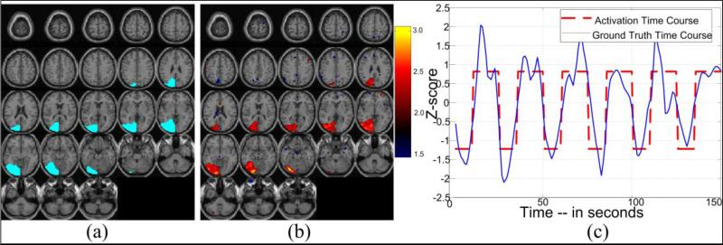
Finally, the spatial component corresponding to the activation was determined by correlating the K time components with the source activation waveform from Section 2.1 (also see Fig. 5(c)), and selecting the one with the highest correlation (about R2 > 0.9 in case of all software phantoms used to generate the results). For, spatial analysis and validation purposes, Z-score maps of this activation component are estimated as Zk (see Fig. 5(b)). An example depicting both spatial and temporal representations of an activation component is presented in Fig. 5(b) and 5(c) respectively. The spatial representation of the ground truth is also provided in Fig. 5(a) for better understanding of the shape and spread of the activation region across different slices. This ground truth map corresponds to the artificial activations that were introduced to the baseline data as described in Section 2.1.
Figure 5. An example of the activation component obtained using the proposed method.
(a) ground truth voxels represented as a different color (not Z-scores); (b) spatial Z-score map representing the activation regions as extracted through ICA in the wavelet domain; (c) corresponding time course of the component shown in (b) along with the waveform of the ground truth introduced as activation.
2.4 Performance measures and metrics: MPSM & CPSM
Following the estimation of the activation component of interest using ICA, it is important to compare its spatial and structural characteristics with that of the ground truth in order to validate the performance of our proposed framework. With this objective, we propose two new structural metrics to quantify the structure integrity maintained by a group of voxels after being processed and classified as an activation region. The first metric, multi-view perimeter shape metric (MPSM) is the mean squared error (MSE) between the perimeter of an activation region for an observation and the ground truth. The second metric is the centroid-based polar shape metric (CPSM) which utilizes a weighted approach by locating voxels that are similar or different in terms of their physical location as compared to the ground truth. The differences are quantized as changes in the radial location or angle with respect to the centroid of a closed shape in a slice-by-slice manner. The CPSM values are reported as the sum of weighted differences in all slices.
2.4.1 Multi-view Perimeter based Shape Metric (MPSM)
The first performance evaluation metric proposed in this paper is based on the underlying fact that activation components have closed surface ROIs. The primary advantage of this metric lies in its ability to quantify the shape of a 3-D polygon using three different estimates computed using perimeters of slices extracted along the axial, coronal and sagittal viewing geometries. This results in a more robust measure of shape congruence as compared to measures estimated using only a single viewing geometry.
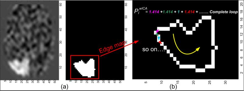
An ROI extends in all three dimensions forming a non-rigid shape that represents the activation voxels. The Z-score volumetric image (Zk) is thresholded using an empirical threshold value (Z-value >= 2.0) to obtain the binary map of ROI (as seen in Fig. 6(a)) for each observation. The empirical threshold was computed using an ROC analysis explained in Section 3. This binary map is known as ZB (index k is ignored from here on). The perimeter of a non-rigid shape is defined as the sum of Euclidean distance between all pairs of adjacent voxels. Let ZB,edge be the binary edge map of the largest contiguous region which is utilized for estimation of the perimeter values as shown in Fig. 6(b). Three different sets of perimeter values corresponding to three orthogonal viewing angles – (1) Axial, (2) Sagittal, and (3) Coronal, were estimated in a slice-by-slice manner. This resulted in three variable length vectors (1×Li) populated by the perimeter values, known as (index i corresponds to the aforementioned viewing angles). Note that, L is of variable length as the extent of spread of non-zero voxels (ZB = 1) across slices is not necessarily equal for different viewing angles.
Figure 6. Generation of a binary edge map and illustration of the proposed perimeter metric.
(a) Slice no.12 of Zk and the corresponding ZB image; (b) Enlarged edge map ZB,edge and perimeter estimation. All pixel pairs oriented at an angle of 45°, 135°, 225° or 315° has , whereas all other pixel pairs have a perimeter = 1.
The aforementioned process was repeated on the Z-score maps estimated through s-ICA and the available ground truths, resulting in two additional sets of perimeter vectors - and respectively. For comparison purposes, is utilized as the reference set, whereas and are considered as the test sets. Further, the MSE value for each comparison pair ( and ) is calculated for each of the three viewing angles mentioned previously. The generalized MSE equation is represented as:
| (6) |
It can be inferred from the above discussion that the metric takes lower values when perimeters of most slices in group G (w-ICA or s-ICA) are almost equal to those of the ground truth.
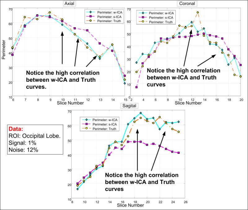
Fig. 7 depicts the perimeter distributions along the set of slices associated with three viewing angles for an example data set. Notice the high correlation between the w-ICA (cyan) and the ground truth (orange) perimeter values. This observation corroborates our previous statement about preservation of shape, that is, directional and spatial relationships between adjacent pixels are quite intact even after de-noising using wavelets in addition to performing ICA in the transform domain. Whereas, there are large differences between perimeters of s-ICA maps and ground truth for every viewing angle, eventually leading to higher values of . More results explaining the above statements are presented in Section 3 of this paper.
Figure 7. Plots depicting perimeter variation between w-ICA and s-ICA for different viewing angles.
High correlation is seen between the curves for ground truth and the w-ICA scheme as compared to the s-ICA framework. This preliminary analysis establishes the significance of slice by slice comparison of perimeters in various viewing geometries. Coronal MSE values for this ROI show the most deviation from ground truth with reasons discussed in Section 3.1.
2.4.2 Centroid based Polar Shape Metric (CPSM)
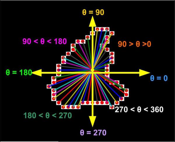
In this section, we introduce a novel weighted metric estimated from a given shape by utilizing polar distances and orientations of several pixels on its contour. Centroid based measures have been previously utilized in combination with b-splines for applications in object recognition and detection (Gaborski and Paskali, 2007; Saber et al., 2005), but there have only been a few attempts made to quantify the shape of activations in fMRI data. With this note, we propose the second shape metric in this paper, termed as the CPSM. Every pixel in a slice ∈ R2 sub-space and can be described by polar co-ordinates (r, θ) computed with respect to another location in the same sub-space. This metric records the amount of change in these (r, θ) values (with respect to ground truth) for every pixel belonging to the outermost contour of an activation region highlighted by the component of interest post-ICA. The initial estimates corresponding to a particular slice are obtained in form of MSE values for Euclidean distances and arctangent angles with respect to the reference centroid (ground truth). In order to keep the distance (r) and angle (θ) estimates unbiased, we utilize the Centroid of the ground truth (Truth) to compute the distances and angles for the test shapes (s-ICA or w-ICA). We provide here, a step-by-step description of the algorithm followed by an illustration in Fig. 8.
Figure 8. Illustration for computation of rotational and translational errors in each quadrant as explained in Steps 3 – 5.
Vectors from the Centroid to each pixel are depicted in different colors along with clearly labeled axes. Various angular quadrants are also labeled for better understanding of the angular errors and decision criteria.
CPSM Algorithm
STEP 1: Initiate the algorithm with ZB,edge maps - ,, as the inputs. Estimate the variable size vectors containing locations of edge pixels in the ith axial slice: ,,.
STEP 2: Compute the Centroid coordinates for each slice - through .
STEP 3: Estimate the Euclidean distance-angle (r, θ) pairs for each pixel in ,,and, with as reference, stored as , and .
STEP 4: Locate /count the pixels in and whose (r, θ) match perfectly with pixels in in a pair wise manner. The total count of these pixels is termed as the gain - and .
STEP 5: Locate/count the pixels in and whose r estimates match perfectly with pixels in . Thus, these pixels contribute to rotational (angle) error, given they are in the same angular quadrant (See Fig. 9). This error primarily accounts for all pixels that have shifted away from the line joining it to the centroid. For example, if a set of corner pixels (ground truth) are rotated (test shape) by an arbitrary angle due to smoothing/denoising operations, it would be recorded as a rotational error. These errors are recorded in form of MSE values ( and ) for each slice i:
| (7) |
where k ∈ (1,2,3,....., Nerr) corresponds to the indices of pixels with a rotational error in slice i.
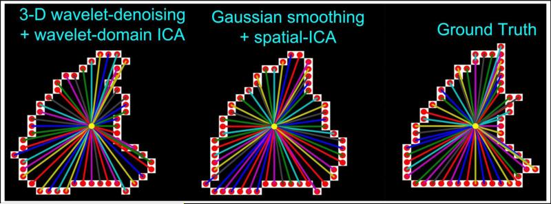
Figure 9. Illustration of difference in shapes and how the distances and angle errors account for this change.
The shapes correspond to slice no. i=10 from , and edge maps. The centroid location for each slice in the ground truth map was used as the centroid location in the other two maps.
STEP 6: Locate /count the pixels in and whose θ estimates match perfectly with pixels in . Thus, these pixels contribute to translational (distance) errors that may have occurred due a pixel moving along the line joining it to the centroid. These errors account for pixel translations occurring due to smoothing/denoising operations, essentially increasing the spatial extent of a particular region in the shape. These errors are recorded in form of MSE values ( and ) for each slice i:
| (8) |
where k ∈(1,2,3.....Nerr) corresponds to the indices of pixels with a translational error in slice i.
STEP 7: Count the number of pixels in and that have neither a distance match nor an angle match with any of the pixels in . This count is stored as a penalty: or . This error accounts for a large shift of several pixels or addition of a false contour due to smoothing/denoising in some region(s) of the image.
From here on the “Truth’ subscript will not appear in any equations as it was absorbed by the MSE equations.
After having obtained four features for each slice and each method (, , and ), in the form of four vectors, we proceed to estimate a weighted combination of these in order to represent the shape of a volume with a single number. We initiate this process by projecting each feature vector to a normalized sub-space by scaling each element with maximum value within that vector, resulting in values ranging between 0 and 1. Further, the normalized feature vectors , , and are accumulated through a weighted sum across each slice resulting in a metric for each slice (see Eqn. 9). This final metric value (CPSMwICA) for the given volume is computed by summing across the aforementioned weighted metric vector.
| (9) |
The above CPSM metric for a given slice is expected to have a low value when the number of perfect matches () is high and value of penalty () is low in addition to low values for errors - and . The coefficients/weights were set based on the significance of the type of error. Perfect matches are always weighted the highest and assigned as the denominator, eventually removing any bias that could be introduced due to a high number of penalty pixels for a given slice. On the contrary, if a slice is severely different from the reference shape, then it is expected to have high distance and angle errors, in addition to high number of penalty pixels resulting in a high CPSM value and less number of perfectly matching pixels. It was observed that the proposed w-ICA framework outperformed the widely applied s-ICA methodology for all test data sets, that is, any signal + noise combination.
These metrics were tested on the simulated data sets as the ground truths were available only for the same and not for real fMRI data. This metric may be applied to real data sets depending on the amount of confidence associated with the accuracy of estimated ground truth shapes, even though the exact spread of the activation in a real fMRI data set is unknown. Amongst their application for quantifying shape congruence, these metrics may be utilized for measuring and quantifying inter-subject variability for various group studies. For example, the difference between the spatial characteristics of activation regions may be estimated for subjects belonging to the same group (healthy controls or diseased subjects) on an absolute scale or for quantification of inter-group variability on a relative scale to compare subjects from different groups.
3. RESULTS & DISCUSSION
The results from the proposed denoising/w-ICA framework were benchmarked against those obtained through the conventionally used FWHM Gaussian smoothing/s-ICA methodology.
In order to furnish a fair indication of the overall performance of our proposed framework, ROC curves were estimated for sixteen data sets artificially generated through all possible combinations of ROIs (Temporal and Occipital Lobe), signal (1% and 3%) and noise levels (6%, 8%,10%, and 12%) as explained previously in Section 2.1. Each of these data sets is comprised of 23 slices per volume and 150 time points, thus resulting in a single spatio-temporal image of size 53×63×23×150. In addition, to understand and quantify the effect of the random distribution of noise in the data sets, we generated 10 spatio-temporal images for every unique combination of the above parameters {signal + noise (n)} where noise (n) corresponds to a random noise frame. Effectively, the complete software phantoms data set is comprised of a total of 160 spatio-temporal volumetric images (16 unique combinations × 10 noise frames per combination). This experiment allowed us to determine an unbiased estimate representing the performance of each algorithm, as discussed in this section.
For the purpose of obtaining the comparative de-noised data corresponding to the widely used Gaussian-based method, we applied an 8×8×8 mm3 FWHM Gaussian kernel built in the SPM package (Poline et al., 1997) . This was followed by estimation of the activation components using the GIFT toolbox (Rachakonda et al., 2007), and the final Z-score maps for each smoothed data set.
3.1 Occipital lobe (or Visuo-motor)
This ROI was selected based on its complex shape in terms of contours and edges in addition to its correspondence with visual tasks that stimulate the Visuo-motor in case of real fMRI experiments.
3.1.1 ROC Analysis
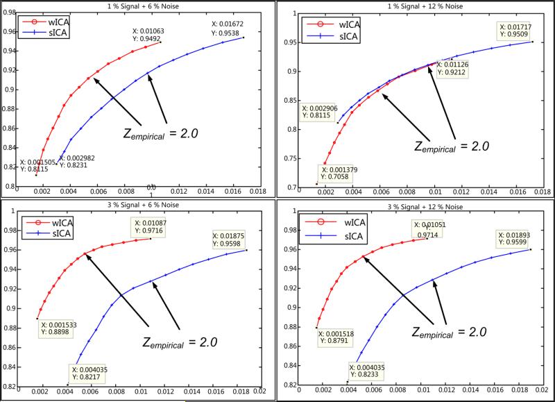
ROC curves were estimated by utilizing the activation component Z-maps for all data and the results are presented in Table 1. For better understanding, the ROC curves corresponding to the lowest and highest noise levels (6% and 12%) are shown in Fig. 10. These curves were generated using Z-values in steps of 0.1 within the threshold interval ~ (1.5, 3.0). In order to fairly represent the TPR and FPR values, an empirical Z-threshold value was obtained using the data set with highest noise content (~ 1% signal, 12 % noise). There is not an imperative requirement for an empirical threshold, as seen in Fig. 10, but in order to numerically present the performance difference between the two methods (see Table 1), we carefully choose an empirical threshold which helps capture a good estimate of this difference. This empirical threshold was set to Zempirical = 2.0 and used across all occipital lobe data sets for estimation of the TPR and FPR values. Further, the thresholded binary map is utilized as input to estimate the values of the proposed shape metrics.
Table 1.
ROC statistics depicting the mean and std. deviations for 10 random noise frames generated for each combination of signal and noise: (a) Signal level = 1%: an improvement of about 2 - 3% for the TPR and 0.7 - 1% for FPR is observed for w-ICA; (b) Signal level = 3%: The TPR and FPR values remain almost constant for varying noise levels with w-ICA outperforming s-ICA in every case above.
| Signal Level = 1% | Signal Level = 3% | ||||||||||
|---|---|---|---|---|---|---|---|---|---|---|---|
| Method | ROC | 6% Noise | 8% Noise | 10% Noise | 12% Noise | Method | ROC | 6% Noise | 8% Noise | 10% Noise | 12% Noise |
| w-ICA | TPR % | 89.3 ± 0.3 | 88.4 ± 0.4 | 88.3 ± 0.6 | 87.5 ± 0.4 | w-ICA | TPR % | 90.91 ± 0.08 | 90.86 ± 0.11 | 90.78 ± 0.13 | 90.31 ± 0.18 |
| FPR % | 0.3 ± 0.03 | 0.31 ± 0.04 | 0.37 ± 0.07 | 0.41 ± 0.09 | FPR % | 0.41 ± 0.02 | 0.39 ± 0.02 | 0.39 ± 0.02 | 0.29 ± 0.02 | ||
| s-ICA | TPR % | 86.7 ± 0.2 | 86.51 ± 0.2 | 86.3 ± 0.2 | 86.1 ± 0.37 | s-ICA | TPR % | 87.29 ± 0.17 | 87.15 ± 0.11 | 87.14 ± 0.07 | 87.09 ± 0.1 |
| FPR % | 1.06 ± 0.07 | 1.21 ± 0.03 | 1.22 ± 0.08 | 1.39 ± 0.04 | FPR % | 1.3 ± 0.03 | 1.3 ± 0.02 | 1.29 ± 0.02 | 1.3 ± 0.01 | ||
| (a) | (b) | ||||||||||
Figure 10.
ROC curves with indication of empirical threshold for two signal levels (1%: top row, 3%: bottom row) and two selected noise levels (6%: left column, 12%: right column) used. Curves for w-ICA show consistently lower FPR for any signal/noise combination (see discussion).
Note that, a single data point on any curve in Fig. 10 corresponds to the mean of true positive rate (TPR) or false positive rate (FPR) value across 10 noise frames at a threshold in interval ~ (1.5, 3.0). These mean and corresponding standard deviations are reported in Table 1.
It is evident from Fig. 10 and Table 1 that the proposed w-ICA framework performs better in terms of classifying activation voxels as compared to the existing framework (s-ICA) for this ROI. These improvements are a direct result of applying and utilizing the selective smoothing abilities of wavelets (preserving edges) and the novel multi-directional denoising technique adopted in this paper. As mentioned in Section 2.2, the multi-directional de-noising scheme applied on each voxel for three different geometries helps prepare a more accurate estimate for signal separation as compared to the spatial smoothing schemes involving 3-D Gaussian smoothing kernels.
The value of TPR and FPR vary with varying noise levels. As the amount of noise increases, the TPR is expected to decrease, but more importantly the FPR is expected to significantly increase due to a greater number of voxels being misclassified. In the case where the diagnostic criterions between two groups of subjects are the spatial extent of an activation region or the accuracy of its shape, ability to achieve low number of false positive voxels is an imperative requirement. The proposed framework is able to achieve this with ease and facilitates in avoiding high FPR even when applied to data with SNR as low as 11 dB (1% signal, 12% noise). As the noise is increased for signal level ~ 1%, the TPR for w-ICA reduced by less than 2% whereas the FPR only increased from 0.3% to about 0.4% (an increase of about 40 voxels).
The results for the s-ICA framework are close to the theoretical expectation, where the TPR and the FPR do not vary significantly with increasing noise levels due to the high spatial smoothing property of FWHM kernels. An essential requirement of any denoising/classification algorithm is to produce least number of false positives while being able to produce a greater number of true positives. To this effect, s-ICA was outperformed consistently by the proposed w-ICA technique with it yielding about 200 to 400 less false positives on an average for all combinations of signal levels (1%, and 3%) and noise (6%, 8%, 10%, and 12%).
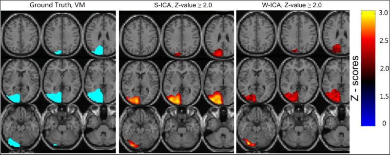
Another interesting characteristic of results is observed with regard to the maintenance of intensity integrity in the spatial component maps across most voxels associated with the activation regions obtained through the w-ICA framework. Whereas in results obtained through the s-ICA framework, the activation regions consist of high valued voxels towards the center (see Fig. 11). This is a direct result of crude spatial smoothing using FWHM Gaussian kernels where the nearby voxels which do not represent the ROI are taken into account while smoothing, thus resulting in higher values and more false positives (as depicted in Fig. 11). This added advantage of w-ICA may play a useful role when analyzing functional connectivity of default mode networks through spatial correlations and overlap. A great deal of research has been done to understand spatial patterns of inter-correlation between underlying cognitive networks in absence of task-evoked activity (Calhoun et al., 2009a; Calhoun et al., 2009b). For example, an arbitrary voxel with high Z-score value (or any other statistic) within an activation region is utilized in connectivity analysis for establishing functional relationships. Spatial correlation analysis may incidentally indicate strong connectivity due to the high Z-score associated with this voxel but ground truth may indicate otherwise. Effectively, this may lead to a large bias and sometimes even false connections when performing a study on a group of subjects. However, the proposed w-ICA framework combined with our 3-D wavelet denoising approach is expected to perform better by facilitating the elimination of such a bias.
Figure 11. Illustration of another advantage of the w-ICA framework over s-ICA (1% signal + 12% noise).
showing the integrity of intensities across the activation region. The image for s-ICA shows centrally bright areas due to its high spatial smoothing properties. The image for w-ICA has more or less uniform values throughout the activation region as originally introduced in form of the ground truth. The ROI highlighted in ground truth is label map in contrast to the Z-score maps presented for s-ICA and w-ICA.
3.1.2 Shape metrics for occipital lobe
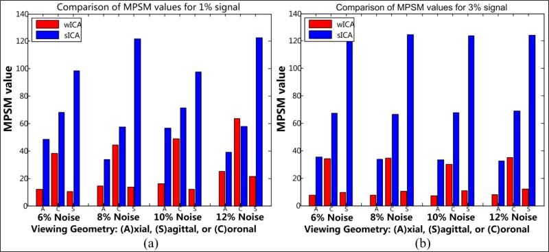
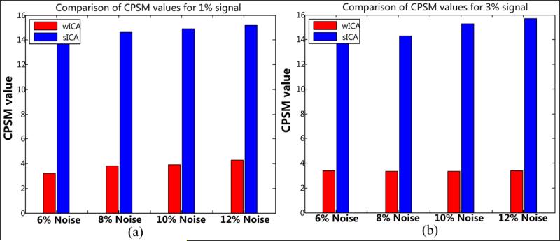
As a continuation to the above discussion, we present the next set of results related to the shape metrics introduced previously in Section 2.4. These metrics are found to be useful evaluation tools that effectively highlight the high level of shape distortions caused due to crude smoothing while indicating the advantage of 3-D wavelet based approach. The MPSM and CPSM results for this ROI are summarized in Tables 2 and 3 in addition to graphical representations presented in Fig. 12 and 13 respectively.
Table 2.
Occipital lobe: MPSM statistics reported here as the mean and standard deviations of MSEwICA–Truth and MSEsICA–Truth (Eqn. 6) for each viewing angle. The mean and standard deviation values were computed using MSE values across 10 noise frames for every possible signal/noise combination: (a) signal = 1%; (b) signal = 3%. Note that the level of shape congruence is inversely proportional to the metric values. The metric acquires low values if the shape is more similar to the ground truth and vice versa.
| MPSM - Signal Level = 1% | MPSM - Signal Level = 3% | ||||||||||
|---|---|---|---|---|---|---|---|---|---|---|---|
| Method | Viewing Geometry | 6% Noise | 8% Noise | 10% Noise | 12% Noise | Method | View | 6% Noise | 8% Noise | 10% Noise | 12% Noise |
| w-ICA | Axial | 11.99 ± 3.83 | 14.7 ± 5.22 | 16 25 ± 6.38 | 25.06 ± 11.93 | w-ICA | Axial | 7.73 ± 1 38 | 7.64 ± 0.44 | 7 26 ± 1.34 | 7.91 ± 2.16 |
| Coronal | 38.33 ± 12.84 | 44.32 ± 16.54 | 49.07 ± 31.1 | 63.7 ± 17.11 | Coronal | 34.37 ± 10.38 | 34.64 ± 17.41 | 30.25 ± 11.97 | 34.92 ± 9.05 | ||
| Sagittal | 10.42 ± 3.11 | 13.66 ± 4.46 | 11.98 ± 6.1 | 21.48 ± 11.8 | Sagittal | 9.72 ± 2.41 | 10.37 ± 2.89 | 10.72 ± 2.37 | 12.23 ± 3.15 | ||
| s-ICA | Axial | 48.54 ± 9.39 | 33.74 ± 5.34 | 56.85 ± 17.2 | 39.02 ± 9.54 | s-ICA | Axial | 35.28 ± 3.23 | 33.86 ± 1.97 | 33.51 ± 1.89 | 32.48 ± 2.3 |
| Coronal | 68.16 ± 7.25 | 57.45 ± 9.3 | 71.32 ± 8.87 | 57.83 ± 8.88 | Coronal | 67.42 ± 2.17 | 66.59 ± 3.2 | 67.71 ± 1.47 | 69.04 ± 1.25 | ||
| Sagittal | 98.53 ± 6.63 | 121.98 ± 5.94 | 97.52 ± 13.19 | 122.71 ± 9.91 | Sagittal | 123.74 ± 3.8 | 124.76 ± 2.96 | 123.73 ± 2.57 | 124.12 ± 1.52 | ||
| (a) | (b) | ||||||||||
Table 3.
Occipital lobe: CPSM statistics computed similar to Table 2 and reported as mean and standard deviations of CPSMwICA and CPSMsICA values across 10 noise frames for every possible combination: (a) signal = 1%; (b) signal = 3%. Note that the level of shape congruence is inversely proportional to the metric values. The metric acquires low values if the shape is more similar to the ground truth and vice versa.
| CPSM - Signal Level = 1% | CPSM - Signal Level = 3% | ||||||||||
|---|---|---|---|---|---|---|---|---|---|---|---|
| Method | Viewing geometry | 6% Noise | 8% Noise | 10% Noise | 12% Noise | Method | Viewing geometry | 6% Noise | 8% Noise | 10% Noise | 12% Noise |
| w-ICA | Axial | 3.21 ± 0.32 | 3.79 ± 0.34 | 3.92 ± 0.71 | 4.28 ± 0.53 | w-ICA | Axial | 3.37 ± 0.02 | 3.36 ± 0.23 | 3.35 ± 0.18 | 3.41 ± 0.36 |
| s-ICA | Axial | 14.39 ± 0.85 | 14.6 ± 1.41 | 14.88 ± 3.53 | 15.17 ± 2.9 | s-ICA | Axial | 13.85 ± 0.96 | 14.27 ± 0.98 | 15.29 ± 0.82 | 15.69 ± 0.85 |
| (a) | (b) | ||||||||||
Figure 12. Occipital lobe.
Bar plots depicting the difference between the mean MPSM values presented in Table 2: (a) signal = 1%; (b) signal = 3%. The bars are grouped based on different levels of noise and three different viewing geometries as indicated in Table 2.
Figure 13. Occipital Lobe.
Bar plots depicting the difference between the mean CPSM values presented in Table 2: (a) signal = 1%; (b) signal = 3%. The bars are grouped based on different levels of noise depicted in Table 3.
The MPSM and CPSM values were estimated across 10 noise frames and the results are reported here as their mean and standard deviations. Large number of discontinuous contours in some of the coronal slices and relatively lower smoothing properties of w-ICA (as compared to s-ICA) resulted in large variance values as seen in Table 2 above. An interesting observation regarding the measurements for coronal geometry was that there were multiple instances with more than one closed contour in a single slice for the ground truth. Binary maps each obtained from w-ICA and s-ICA result in a more dilated version of the closed contours due to the smoothing process, sometimes resulting in only one closed region instead of multiple regions as originally present in the ground truth. The s-ICA method is more susceptible to this error (as seen from large mean values in Table 2), but shows lower variance due to its significant smoothing properties. In most cases, w-ICA was able to maintain the isolation between multiple regions within a slice (if present) resulting in lower mean MPSM values.
The next set of results is based on the CPSM described in Section 2.4. The MPSM primarily focuses on the spread of the contours as a whole whereas CPSM takes into account the shape of the contour on a pixel-by-pixel basis. The CPSM values for the occipital lobe (see Table 3) quantify the difference between the two methods on a pixel-by-pixel basis across 10 noise frames. A significant and consistent improvement is observed for the w-ICA method with low variance as seen from Table 3 and Fig. 13. Note that CPSM is estimated using axial geometry only. This is simpler to interpret as most diagnostic analyses are done using axial slices. Although, a more accurate estimate of CPSM may be obtained by using 3-D spherical coordinates for the estimation of the centroid. Also, solid angles may be computed for different regions belonging to the surface of 3-D non-rigid activation region.
3.2 Temporal lobe
This particular ROI was selected based upon the fact that it contains large number of voxels. Large spatial smoothing kernels introduce a significant amount of smoothing which may be harmless or sometimes even beneficial when the size of ROI is large as their shapes tend to vary gradually leading to lower variability after smoothing. The ROC statistics presented in this section corroborate the above statement to some extent. This may be inferred from the fact that the s-ICA framework performs competitively well against the w-ICA framework by resulting in a larger number of true positives. Although, when the shape of an ROI varies rapidly, which is the case for some of the slices in the temporal lobe, then smoothing with a spherical Gaussian would not be a robust choice and would tend to destroy the edges. Thus, s-ICA fails to preserve the overall shape of an activation region in addition to large number of misclassified voxels. Given the aforementioned case, the shape metrics facilitate in validation of the statement that there exists closer shape congruence in case of w-ICA results as compared to s-ICA output.
3.2.1 ROC statistics
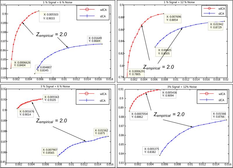
The ROC curves for two extreme noise levels (Zempirical = 2.0) presented in Fig. 14 clearly show that w-ICA assists in establishing a highly desirable requirement of low number of false positives for neuroimaging applications. The ROC curves for the w-ICA method yielded higher TPRs and lower FPRs, given a higher percentage of simulated BOLD signal (~ 3%), whereas w-ICA performed competitively well against s-ICA when compared for 1% BOLD signal change. The TPR values of w-ICA differ by a small percentage whereas a significant improvement is evident from the FPR values, as compared to s-ICA at every given noise level (also seen from Table 4).
Figure 14.
ROC curves with indication of empirical threshold for two signal levels (1%: top row, 3%: bottom row) and two selected noise levels (6%: left column, 12%: right column) used. In all cases above and as presented in Table 4 also, the number of false positives always remains lower for w-Ica as compared to s-ICA. The TPR is competitive for 1% signal and higher for 3% for w-ICA against s-ICA.
Table 4.
ROC statistics depicting the mean and std. deviations of TPR and FPR for 10 random noise frames generated for each combination of signal and noise: (a) Signal level = 1%; (b) Signal level = 3%. Clearly, w-ICA shows superior statistics for all combinations except lower TPR for 1% signal and higher levels of noise.
| ROC - Signal Level = 1% | ROC - Signal Level = 3% | ||||||||||
|---|---|---|---|---|---|---|---|---|---|---|---|
| Method | ROC | 6% Noise | 8% Noise | 10% Noise | 12% Noise | Method | ROC | 6% Noise | 8% Noise | 10% Noise | 12% Noise |
| w-ICA | TPR % | 91.89 ± 0.65 | 90.83 ± 0.73 | 89.3 ± 0.7 | 86.67 ± 0.8 | w-ICA | TPR % | 96.1 ± 0.12 | 96 ± 0.18 | 95.9 ± 0.18 | 95.77 ± 0.34 |
| FPR % | 0.602 ± 0.02 | 0.57 ± 0.03 | 0.59 ± 0.03 | 0.58 ± 0.04 | FPR % | 0.62 ± 0.02 | 0.61 ± 0.03 | 0.6 ± 0.02 | 0.61 ± 0.03 | ||
| s-ICA | TPR % | 92.43 ± 0.35 | 92.09 ± 0.65 | 91.15 ± 0.43 | 91.1 ± 0.63 | s-ICA | TPR % | 93.54 ± 0.16 | 93.49 ± 0.16 | 93.47 ± 0.16 | 93.44 ± 0.12 |
| FPR % | 1.05 ± 0.02 | 1.05 ± 0.05 | 1.25 ± 0.03 | 1.26 ± 0.39 | FPR % | 1.2 ± 0.02 | 1.21 ± 0.02 | 1.21 ± 0.02 | 1.21 ± 0.02 | ||
| (a) | (b) | ||||||||||
The effect of increasing noise levels on ROC statistics is markedly visible from the values in Table 4 (a). The TPR values for w-ICA show a significantly decreasing trend (~ 4% reduction for signal level = 1%) as noise increases, in comparison to s-ICA. The advantage of w-ICA lies in restricting the false positives, in this case, below 1% for any given signal and noise combination. On an average, an improvement of about 150-200 voxels (equivalent to ΔFPR ~ 0.5 – 0.7 %) is observed for w-ICA results. This difference is expected to be significantly high when the data is acquired at a finer resolution in comparison to current 3×3×3mm sampled resting state fMRI data set. In case the signal level is high (~ 3%), the w-ICA technique is able to achieve TPR and FPR values much greater than those obtained using the s-ICA method (see Fig. 14 (bottom row), Table 4(b)).
3.2.2 Shape metrics for temporal lobe
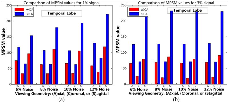
The second set of results presented in this section corresponds to the values associated with proposed shape metrics – MPSM (Table 5 and Fig. 16) and CPSM (Table 6 and Fig. 17). As expected, the s-ICA framework introduces large number of false positives around the activation region. This directly causes a large amount of shape distortion and is demonstrated here.
Table 5.
Temporal lobe: MPSM statistics reported here as the mean and standard deviations of MSEwICA–Truth and MSEsICA–Truth (Eqn. 6) for each viewing angle. The mean and standard deviation values were computed using MSE values across 10 noise frames for every possible signal/noise combination: (a) signal = 1%; (b) signal = 3%.
| MPSM - Signal Level = 1% | MPSM - Signal Level = 3% | ||||||||||
|---|---|---|---|---|---|---|---|---|---|---|---|
| Method | View | 6% Noise | 8% Noise | 10% Noise | 12% Noise | Method | View | 6% Noise | 8% Noise | 10% Noise | 12% Noise |
| w-ICA | Axial | 74.76 ± 13.07 | 62.63 ± 6.98 | 66.44 ± 21.71 | 58.99 ± 15.76 | w-ICA | Axial | 66.26 ± 2.74 | 66.75 ± 3.6 | 69.21 ± 4.04 | 69.4 ± 7.46 |
| Coronal | 33.74 ± 4.36 | 34.34 ± 8.2 | 34.37 ± 8.54 | 38.34 ± 6.33 | Coronal | 25.35 ± 2.37 | 19.18 ± 2.69 | 20.71 ± 3.38 | 22.54 ± 4.01 | ||
| Sagittal | 97 ± 18.56 | 110.85 ± 20.5 | 105.76 ± 24.68 | 118.93 ± 29.15 | Sagittal | 79.59 ± 4.05 | 79.67 ± 7.68 | 86.45 ± 10.46 | 90.92 ± 10.28 | ||
| s-ICA | Axial | 117.02 ± 3.69 | 107.14 ± 10.5 | 106.48 ± 5.66 | 130.67 ± 5.38 | s-ICA | Axial | 126.45 ± 4.16 | 127.37 ± 2.22 | 126.64 ± 4.54 | 128.87 ± 7.06 |
| Coronal | 64.76 ± 2.58 | 62.98 ± 5.68 | 62.86 ± 3.56 | 82.93 ± 2.47 | Coronal | 71.12 ± 1.81 | 71.07 ± 1.42 | 71.22 ± 1.15 | 70.78 ± 2.07 | ||
| Sagittal | 153.86 ± 17.86 | 179.47 ± 27.01 | 194.44 ± 14.42 | 221.49 ± 17.53 | Sagittal | 236.74 ± 5.97 | 232.1 ± 11.63 | 229.47 ± 13.66 | 229.84 ± 19.86 | ||
| (a) | (b) | ||||||||||
Figure 16. Temporal lobe.
Bar plots depicting the difference between the mean MPSM values presented in Table 5: (a) signal = 1%; (b) signal = 3%. The bars are grouped based on different levels of noise and three different viewing geometries as indicated in Table 5. Large values and large differences are observed along the sagittal geometry for any given signal/noise combination.
Table 6.
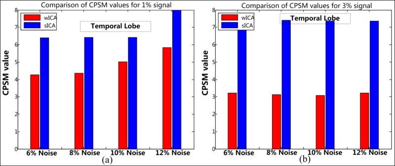
Temporal lobe: CPSM statistics computed for temporal lobe data reported as mean and standard deviations of CPSMwICA and CPSMsICA values across 10 noise frames for every possible combination: (a) signal = 1%; (b) signal = 3%. The number of perfect matches or Gain (weighted highest in CPSM) is high in case of a large ROI such as the temporal lobe. This directly results in lower values for CPSM for s-ICA as compared to values observed in case of occipital lobe in Table 3.
| CPSM - Signal Level - 1% | CPSM - Signal Level = 3% | ||||||||||
|---|---|---|---|---|---|---|---|---|---|---|---|
| Method | Viewing geometry | 6% Noise | 8% Noise | 10% Noise | 12% Noise | Method | Viewing geometry | 6% Noise | 8% Noise | 10% Noise | 12% Noise |
| w-ICA | Axial | 4.26 ± 0.29 | 4.36 ± 0.5 | 5.01 ± 0.43 | 5.83 ± 0.52 | w-ICA | Axial | 3.08 ± 0.15 | 3.12 ± 0.2 | 3.21 ± 0.11 | 3.22 ± 0.2 |
| s-ICA | Axial | 6.4 ± 0.55 | 6.42 ± 0.5 | 6.42 ± 0.56 | 7.99 ± 0.32 | s-ICA | Axial | 7.39 ± 0.25 | 7.41 ± 0.27 | 7.36 ± 0.29 | 7.36 ± 0.29 |
| (a) | (b) | ||||||||||
Figure 17. Temporal lobe.
Bar plots depicting the difference between mean CPSM values presented in Table 6: (a) signal = 1%; (b) signal = 3%. The bars are grouped based on different levels of noise depicted in Table 6. For 3% signal level, both frameworks perform consistently with increasing noise, whereas larger shape distortion is observed for 1% signal level with increasing level of noise as seen in (a).
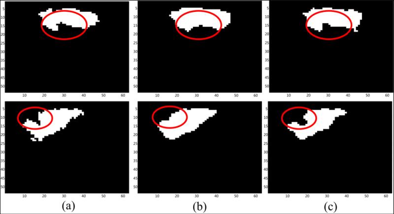
Evidence related to shape distortion caused by smoothing is presented in the form of thresholded Z-score maps of the activation component. Fig. 15 depicts the shape of the resulting Z-score maps for slices 14 and 17, obtained after the application of the s-ICA and the w-ICA frameworks respectively. It is visible that the cusps are preserved (see Fig. 15 (c)) in case of the w-ICA results. Whereas, the shapes change considerably as a result of Gaussian smoothing incorporated in s-ICA (see Fig. 15(b)).
Figure 15. Illustration of variation in shape of the activation region for temporal lobe ROI.
Slice 15 (top row) and slice 17 (bottom row): (a) Ground truth; (b) s-ICA; (c) w-ICA. The areas highlighted above are the most significance regions in context to shape preservation as achieved by w-ICA over s-ICA. Notice that the cusp in slice 17 is smoothed out as a result of s-ICA and preserved by the w-ICA framework. These shape distortions are expected to be even higher when comparing the un-thresholded Z-score maps.
A marked improvement is observed in shape measures for the w-ICA framework in comparison to the s-ICA method. The low MPSM and CPSM values for w-ICA indicate higher shape congruence as seen from Figs. 16 and 17 respectively. The high sagittal MSE values seen in Table 5 are due to the rapidly varying shape of the temporal lobe ROI for this viewing geometry. Also, these large variations may be accounted by multiple instances of more than one closed contour being present in a single sagittal slice for ground truth. These multiple closed regions, when in close proximity, undergo dilation due to smoothing and thus yield high MSE values when compared with the ground truth. The distribution of MPSM values also seem to vary more with increasing noise as inferred from high values of standard deviations in Table 5. In a broader sense, MPSM is capable of yielding a fair estimate of the amount of shape congruence for all three viewing geometries and provides enough information to make a decision about the quality of performance of the two frameworks.
The basis for superior performance of the w-ICA over s-ICA is further bolstered through the CPSM values depicted in Table 6 and bar plots presented in Fig. 17. Temporal lobe being a large ROI consists of more complex contours across different slices. The edges along these contours were found to be spontaneously varying, thus resulting in larger distortion in shapes as a result of spatial smoothing. A larger shift in voxels in terms of (r, θ) measures is observed, in addition to greater numbers of voxels being classified as misses which eventually resulted in larger CPSM values for s-ICA framework that employs Gaussian smoothing and ICA in the spatial domain. Low CPSM values were obtained through w-ICA as the wavelets are known to preserve edges and introduce little amounts of spatial smoothing further enabling the generation of better estimates of independent components through ICA being performed in the wavelet domain.
Conclusively, for any given level of signal or noise, w-ICA seems to maintain higher overall shape congruence (lower CPSM and MPSM values), in addition to superior ROC statistics (higher TPR and lower FPR) for various levels of signal and noise.
3.3 Real fMRI data (motor tapping)
For the purpose of demonstrating the performance of the proposed framework on real data, we utilized a task-related fMRI data set. Both frameworks, w-ICA and s-ICA, were applied to the real data and the results are compared in this section. The data was collected during a block-design motor tapping study which consisted of periods of 30s off time and 30s on time. The subject (healthy control) tapped his right-hand finger during the on period and rested during the off cycle. There were five and a half cycles, starting with an off and ending with an off period. For each subject, 165 whole head fMRI images were collected. The proposed w-ICA framework was applied on the aforementioned real data set of size 53×63×46×165 where the resolution of each voxel ~ 3×3×3 mm3.
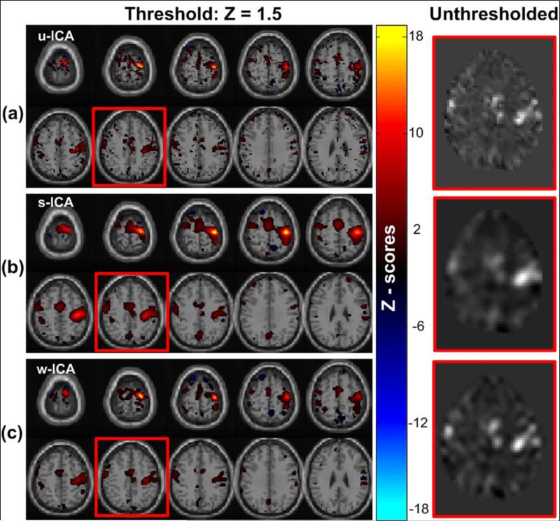
For unbiased comparisons, we also generated results corresponding to ICA algorithm without any type of smoothing being applied to the data. This process is termed as “u-ICA’ or unsmooth ICA. Note that, it is would not be a good practice to treat the u-ICA results as a ground truth, as there is a much more complex process involved in generation of these activations within the brain which is yet to be deciphered with absolute accuracy. The corresponding results for u-ICA, s-ICA, and w-ICA are illustrated in Fig. 18.
Figure 18. Results for motor-tapping fMRI data.
Illustration of the activation components (left) and un-thresholded Z-score maps (right) obtained for (a) unsmooth data and spatial ICA (u-ICA), (b) Gaussian smoothing + spatial-domain ICA, and (c) wavelet denoising + wavelet-domain ICA (w-ICA), from the single subject motor tapping data.
The u-ICA results shown in Fig. 18(a) may be utilized to compare the amount of smoothing introduced by the denoising stage in each of the two methods – s-ICA (Fig. 18(b)) and w-ICA (Fig. 18(c)). It is now evident from the results associated with the software phantoms that our proposed framework (w-ICA) is capable of preserving the true shape without spreading the spatial extent of the activation region. It also plays a role in keeping the number of false positives low as compared to the conventional processing framework (s-ICA). A similar conclusion may be inferred from the discussion on a real data set presented here.
We performed an additional analysis using w-sICA (wavelet domain denoising followed by ICA in the spatial domain). The w-sICA method did not perform as well as the w-ICA approach initially, however the performance improved when we increased the number of components from 30 to 40. This suggests that performing ICA in the wavelet domain is a more efficient approach and can be more clearly understood from the following explanation. The reconstructed data may be thought of as a linear combination of voxel values in the wavelet-sub-bands. The w-sICA method that involves the reconstructed denoised data was unable to separate the activation component from other sources if K was set lower than 40. As per our observations, this is a direct consequence of spatial correlation that exists in the reconstructed data (for w-sICA) in contrast to the wavelet coefficients used for wavelet domain ICA in the w-ICA framework. These observations require further investigation and extensive testing on a larger data set to quantify the aforementioned differences more accurately. We propose to include more evidence corroborating the above statements in future work.
Researchers may benefit significantly through application of our framework to large group data studies where they may be able to obtain accurate activation regions and eventually better correspondences when analyzing for connecting pathways representing functional relationships within the brain.
3.4 Summary
We presented various performance characteristics of the proposed w-ICA algorithm against the existing s-ICA methodology. Overall, the proposed methodology performed significantly better in terms of shape preservation, whereas it yielded competitive results in terms of classified (TPR) and misclassified voxels (FPR) depending upon the size of the ROI under consideration. The ROC statistics for the two methods in case of larger ROIs, such as the temporal lobe (~ 2900 voxels) were observed to be closely competitive, whereas the proposed framework dominated for smaller ROIs such as the occipital lobe (~ 1600 voxels). The reason behind the aforementioned observation may be derived from the size of the FWHM kernel utilized in s-ICA. As the size of this kernel is comparable to the size of the ROI in some of its slices, more false positives are introduced eventually resulting in poorer ROC statistics. This is not the case for larger ROIs such as the temporal lobe, where the additional false positives in s-ICA appear due to high spatial smoothing around the edges. The proposed framework was able to overcome the aforementioned problem, and thus resulted in lower FPR values for any combination of signal and noise.
The FWHM Gaussian smoothing kernel used in the s-ICA framework is expected to introduce a large amount of smoothing given their wide support of 8×8×8 mm3. If a smaller blur kernel (such as of size 4×4×4 or 6×6×6 mm3) is used for smoothing, the aforementioned adverse effects of large blur kernels may reduce to some extent. However, given the non-rigid shapes associated with activation ROIs, smoothing with a spherical shaped kernel such as the Gaussian would destroy the underlying contours (Appendix A) and still result in large false positive rate or lower specificity, although higher than the large kernel case. Also for smaller blur kernels, the level of desired noise suppression would not be achieved, thus resulting in unfulfilled gains from the pre-processing stage. Hence, the advantages of wavelet based methods are convincingly greater in terms of achieving shape accuracy in addition to higher specificity and ability to suppress noise. Also, filtering the fMRI data using a Gaussian smoothing filter to remove noise can reduce the information in the data while reducing the noise, since high-frequency features of the data are filtered. The definition of the denoised mixtures in the wavelet domain reduces the Gaussian contamination of these signals and speeds up the convergence. Thus, transforming the data to wavelet domain enables the ICA module for better separation of the features.
4. CONCLUSIONS
We compared effects of two different fMRI analysis frameworks in two different settings: (1) Multi-directional wavelet based denoising + wavelet-domain ICA and (2) FWHM Gaussian smoothing + spatial-ICA, for artificial data sets generated using task-related BOLD activation signals, resting state real fMRI data set and various combinations of signal percentage (1 and 3%) contaminated by Rician distributed noise (6% to 12%). The testing conditions and signal levels were carefully selected in order to closely relate the results with those obtained for real data sets. The two frameworks (w-ICA vs. s-ICA) were then applied on real fMRI motor tapping data and the results were compared qualitatively demonstrating the superior performance characteristics of w-ICA over s-ICA. A larger data set comprising of more number of subjects is expected to provide more evidence supporting the performance of ICA in the decorrelated wavelet space.
Performance analysis for the two frameworks provides sufficient evidence to state that FWHM kernels significantly alter the spatial shape and extent of the activation regions when applied for denoising fMRI data. We introduced application of multi-view perimeter (MPSM) as a desirable metric for shape comparison in addition to a new weighted shape measure (CPSM). The CPSM takes into account rotational and translational effects of denoising and yields a relative number with respect to the shape of the ground truth. All performance analyses were done taking in account the complex non-rigid shape of an activation region.
Future work may include incorporation of a more robust 3-D shape metric using Z-score estimates of the activation components (instead of binary thresholded maps) as well as application of the proposed framework on real fMRI data sets collected for several subjects. As mentioned earlier, advantages of the proposed framework are expected to be even greater when the number of subjects is large and we plan to show this with sufficient evidence in our future work.
APPENDIX A
Wavelets vs. FWHM Gaussian filters: The impact on shape of activations
Generally smoothing removes high frequency content and details and retains low frequency (with blurring) information. Traditional smoothing filters such as mean, median and Gaussian filters normally employed in the spatial domain smooth the signals with blurring effects and consequently result in loss of edge details. When the primary requirement of an application is to obtain an ROI with high sensitivity (true positives), it becomes imperative to preserve details such as edges and surface smoothness.
We performed an experiment on the known “Shepp-Logan’ brain phantom available in MATLAB® and added non-rigid ROIs with certain gray values to it. Next, Gaussian noise was added to the above software phantom and is shown in Fig. A-1(a) below. The noisy image was filtered using two methodologies – (1) FWHM Gaussian kernel of size 3×3 voxels, and (2) Proposed wavelet based methodology (explained in the next section). The filtered images obtained from the two methods are illustrated in Fig. A-1(b)-(c).
Figure A-1.
Illustration of comparison between denoising methods: (a) Noisy image with two different ROIs; (b) Filtered image with a 3x3 FWHM Gaussian kernel; (c) Filtered image through wavelet coefficient shrinkage.
Two different ROIs were used to illustrate the performance difference between the two methodologies – (a) ROI-A: circular shape; and (b) ROI-B: a random non-rigid shape. A survey of even a small number of published fMRI papers will demonstrate that activated brain regions typically constitute of volumetric regions with non-rigid shapes that are difficult to describe using known mathematical models. As seen from Fig. A-1 above, Gaussian filtering tends to introduce more false positives (larger spread) without any significant distortion in the shape of ROI-A whereas the congruence between the underlying shapes of ROI-B and the filtered result is almost lost. On the contrary, the filtered image obtained from wavelet-based denoising (Fig. A-1(c)) shows much less spatial spread resulting in lower number of false positives while also reducing the background noise levels. More importantly, wavelets do a much better job at preserving the shape of original ROI in the noisy image; in addition to preservation of edge details and transition in gray levels (see Fig. A-1(a) and A-1(c)).
APPENDIX B
Probabilistic Estimator for Wavelet Coefficient Shrinkage
The estimator requires the conditional probability distributions of the magnitude of wavelet coefficients corresponding to the signal and noise which are mathematically represented by pmk|x̂k (mk | x̂k = 1) and pmk|x̂k (mk | x̂k = 0) respectively, where mk = |wk| for each kth voxel and any arbitrary sub-band D. Empirically, these distributions are obtained by utilizing the histogram distributions of signal and noise voxels in x̂j. Let S0 = {k : x̂k =0} and S1 = {k : x̂k =1} whereas p̂mk|x̂k (mk | x̂k = 0) and p̂mk|x̂k (mk | x̂k = 1) be the empirical estimates computed as the histograms of {mk : k ∈ S0} and {mk : k ∈ S1} respectively.
The second component required for the estimator is termed as the local spatial activity indicator or the expected value indicator Ek which is similar to the one described in (Pizurica et al., 2003). If the signal of interest is surely absent at a particular location k, then yk ≈ 0 which implies that the expected value, E(yk | wk, xk = 0) ≈ 0, hence voxel at location k may be classified as noise. Therefore, the expected value of signal at that location may be written E(yk | wk, xk = 1) ≈ wk which would compensate for the fact that a vast majority of coefficients are above the noise level. Effectively, after applying the Bayes’ theorem, the a priori probability of presence of signal and noise can be expressed as Eqn. (B-1) and (B-2) respectively:
| (B-1) |
| (B-2) |
As described in (Pizurica et al., 2003), the signal estimate may be separated in to two components each corresponding to signal and noise, as expressed in Eqn. (B-3) below:
| (B-3) |
where the second term of the equation approaches zero if the signal of interest is absent. Thus, the above equation may be re-written by applying the Bayes’ theorem and expressed as:
| (B-4) |
| (B-5) |
| (B-6) |
hence, the final estimated value of at level j, is utilized as initialization parameter to compute x̂k for the next finer level j -1 and so on. It was essential to compute a 4 level 3-D SWT in order to perform hierarchical de-noising on details associated with the 3 preceding scales. The wavelet coefficients at level 4 were utilized only for initialization of the de-noising scheme in Eqn. (B-4). Finally, the aforementioned procedure results in denoised estimates at the coarsest level (k = 1) which are then utilized for signal separation.
REFERENCES
- Antonini M, Barlaud M, Mathieu P, Daubechies I. Image coding using wavelet transform. IEEE Transactions on Image Processing. 1992;1:205–220. doi: 10.1109/83.136597. [DOI] [PubMed] [Google Scholar]
- Azzerboni B, Carpentieri M, La Foresta F, Morabito F. Neural-ICA and wavelet transform for artifacts removal in surface EMG. 2004:3223–3228. [Google Scholar]
- Azzerboni B, La Foresta F, Mammone N, Morabito F. A new approach based on wavelet-ICA algorithms for fetal electrocardiogram extraction.. Citeseer; European Symposium on Artificial Neural Networks..2005. pp. 193–198. [Google Scholar]
- Bao P, Zhang L. Noise reduction for magnetic resonance images via adaptive multiscale products thresholding. IEEE transactions on medical imaging. 2003;22:1089. doi: 10.1109/TMI.2003.816958. [DOI] [PubMed] [Google Scholar]
- Boroomand A, Ahmadian A, Oghabian M, Alirezaie J, Beckman C. An Efficient Hybrid Wavelet-ICA algorithm for Analyzing Simulated fMRI Data in Noisy Environment. 2007:408–413. [Google Scholar]
- Breakspear M, Brammer M, Bullmore T, Das P, Williams L. Spatiotemporal wavelet resampling for functional neuroimaging data. Human Brain Mapping. 2004;23:1–25. doi: 10.1002/hbm.20045. [DOI] [PMC free article] [PubMed] [Google Scholar]
- Buckheit J, Chen S, Donoho D, Johnstone I, Scargle J. Wavelab software package version 0.700, Technical Report. Department of Statistics, Stanford University; Stanford, California: 1995. About wavelab. [Google Scholar]
- Bullmore E, Long C, Suckling J, Fadili J, Calvert G, Zelaya F, Carpenter T, Brammer M. Colored noise and computational inference in neurophysiological (fMRI) time series analysis: resampling methods in time and wavelet domains. Human Brain Mapping. 2001;12:61–78. doi: 10.1002/1097-0193(200102)12:2<61::AID-HBM1004>3.0.CO;2-W. [DOI] [PMC free article] [PubMed] [Google Scholar]
- Calhoun V, Adali T, Hansen L, Larsen J, Pekar J. ICA of functional MRI data: an overview. Citeseer. 2003:281–288. [Google Scholar]
- Calhoun V, Adali T, Pearlson G, Pekar J. Spatial and temporal independent component analysis of functional MRI data containing a pair of task-related waveforms. Human Brain Mapping. 2001;13:43–53. doi: 10.1002/hbm.1024. [DOI] [PMC free article] [PubMed] [Google Scholar]
- Calhoun V, Eichele T, Pearlson G. Functional brain networks in schizophrenia: a review. Front. Hum Neurosci. 2009a:3. doi: 10.3389/neuro.09.017.2009. [DOI] [PMC free article] [PubMed] [Google Scholar]
- Calhoun V, Liu J, AdalI T. A review of group ICA for fMRI data and ICA for joint inference of imaging, genetic, and ERP data. NeuroImage. 2009b;45:S163–S172. doi: 10.1016/j.neuroimage.2008.10.057. [DOI] [PMC free article] [PubMed] [Google Scholar]
- Donoho D. De-noising by soft-thresholding. IEEE transactions on information theory. 1995;41:613–627. [Google Scholar]
- Donoho D, Johnstone J. Ideal spatial adaptation by wavelet shrinkage. Biometrika. 1994;81:425. [Google Scholar]
- Frackowiak R. Human brain function. Academic Press; 2004. [Google Scholar]
- Friston K, Holmes A, Worsley K, Poline J, Frith C, Frackowiak R. Statistical parametric maps in functional imaging: a general linear approach. Human Brain Mapping. 1994;2:189–210. [Google Scholar]
- Gaborski R, Paskali J. A Cognitively motivated video detection system. Journal of Applied Science & Engineering Technology. 2007:1. [Google Scholar]
- He L, Greenshields I. A non-local maximum likelihood estimation method for Rician noise reduction in MR images. IEEE transactions on medical imaging. 2009;28:8. doi: 10.1109/TMI.2008.927338. [DOI] [PubMed] [Google Scholar]
- Hilton M, Ogden T, Hattery D, Eden G, Jawerth B. Wavelet processing of functional MRI data. Wavelets in Biology and Medicine. 1996 [Google Scholar]
- Huettel S, Song A, McCarthy G. Functional magnetic resonance imaging. Sinauer Associates; Sunderland, MA: 2004. [Google Scholar]
- Johnson R, Marchini J, Smith S, Beckmann C. Independent component analysis of functional magnetic resonance imaging data using wavelet dictionaries. Independent Component Analysis and Signal Separation. 2007:625–632. [Google Scholar]
- Kadah Y. Adaptive denoising of event-related functional magnetic resonance imaging data using spectral subtraction. IEEE Transactions on Biomedical Engineering. 2004:51. doi: 10.1109/TBME.2004.831525. [DOI] [PubMed] [Google Scholar]
- Lancaster J, Woldorff M, Parsons L, Liotti M, Freitas C, Rainey L, Kochunov P, Nickerson D, Mikiten S, Fox P. Automated Talairach atlas labels for functional brain mapping. Human Brain Mapping. 2000;10:120–131. doi: 10.1002/1097-0193(200007)10:3<120::AID-HBM30>3.0.CO;2-8. [DOI] [PMC free article] [PubMed] [Google Scholar]
- Lang M, Guo H, Odegard J, Burrus C, Wells Jr R. Noise reduction using an undecimated discrete wavelet transform. IEEE Signal Processing Letters. 1996;3:10–12. [Google Scholar]
- Long C, Brown E, Manoach D, Solo V. Spatiotemporal wavelet analysis for functional MRI. NeuroImage. 2004;23:500–516. doi: 10.1016/j.neuroimage.2004.04.017. [DOI] [PubMed] [Google Scholar]
- Mallat S. A theory for multiresolution signal decomposition: The wavelet representation. IEEE transactions on pattern analysis and machine intelligence. 1989;11:674–693. [Google Scholar]
- Mallat S. A wavelet tour of signal processing. Academic Pr. 1999 [Google Scholar]
- McKeown M, Makeig S, Brown G, Jung T, Kindermann S, Bell A, Sejnowski T. Analysis of fMRI data by blind separation into independent spatial components. Human Brain Mapping. 1998;6:160–188. doi: 10.1002/(SICI)1097-0193(1998)6:3<160::AID-HBM5>3.0.CO;2-1. [DOI] [PMC free article] [PubMed] [Google Scholar]
- Middleton D, Esposito R. Simultaneous optimum detection and estimation of signals in noise. IEEE transactions on information theory. 1968;14:10. [Google Scholar]
- Monir S, Siyal M. Denoising functional magnetic resonance imaging time-series using anisotropic spatial averaging. Biomedical Signal Processing and Control. 2009;4:16–25. [Google Scholar]
- Pizurica A, Philips W, Lemahieu I, Acheroy M. A versatile wavelet domain noise filtration technique for medical imaging. IEEE transactions on medical imaging. 2003;22:323. doi: 10.1109/TMI.2003.809588. [DOI] [PubMed] [Google Scholar]
- Pizurica A, Wink A, Vansteenkiste E, Philips W, Roerdink B. A review of wavelet denoising in MRI and ultrasound brain imaging. Current Medical Imaging Reviews. 2006;2:247–260. [Google Scholar]
- Poline J, Worsley K, Evans A, Friston K. Combining spatial extent and peak intensity to test for activations in functional imaging. NeuroImage. 1997;5:83–96. doi: 10.1006/nimg.1996.0248. [DOI] [PubMed] [Google Scholar]
- Rachakonda S, Egolf E, Correa N, Calhoun V. Group ICA of fMRI Toolbox (GIFT) Manual. 2007 [Google Scholar]
- Saber E, Xu Y, Murat Tekalp A. Partial shape recognition by sub-matrix matching for partial matching guided image labeling. Pattern Recognition. 2005;38:1560–1573. [Google Scholar]
- Tabelow K, Polzehl J, Voss H, Spokoiny V. Analyzing fMRI experiments with structural adaptive smoothing procedures. NeuroImage. 2006;33:55–62. doi: 10.1016/j.neuroimage.2006.06.029. [DOI] [PubMed] [Google Scholar]
- Tenmoto H, Kudo M, Shimbo M. MDL-based selection of the number of components in mixture models for pattern classification. Advances in Pattern Recognition. 1998:831–836. [Google Scholar]
- Unser M, Aldroubi A. A review of wavelets in biomedical applications. Proceedings of the IEEE. 1996;84:626–638. [Google Scholar]
- Van De Ville D, Blu T, Unser M. Surfing the brain. IEEE engineering in medicine and biology magazine. 2006;25:65. doi: 10.1109/memb.2006.1607671. [DOI] [PubMed] [Google Scholar]
- Van De Ville D, Seghier M, Lazeyras F, Blu T, Unser M. WSPM: Wavelet-based statistical parametric mapping. NeuroImage. 2007;37:1205–1217. doi: 10.1016/j.neuroimage.2007.06.011. [DOI] [PubMed] [Google Scholar]
- Wink A, Roerdink J. Denoising functional MR images: a comparison of wavelet denoising and Gaussian smoothing. IEEE transactions on medical imaging. 2004;23:374–387. doi: 10.1109/TMI.2004.824234. [DOI] [PubMed] [Google Scholar]
- Xu Y, Weaver J, Healy D, Lu J. Wavelet transform domain filters: a spatially selective noise filtration technique. IEEE Transactions on Image Processing. 1994;3:747–758. doi: 10.1109/83.336245. [DOI] [PubMed] [Google Scholar]


