Dysregulation of working memory and default‐mode networks in schizophrenia using independent component analysis, an fBIRN and MCIC study

Abstract

Deficits in working memory (WM) are a consistent neurocognitive marker for schizophrenia. Previous studies have suggested that WM is the product of coordinated activity in distributed functionally connected brain regions. Independent component analysis (ICA) is a data‐driven approach that can identify temporally coherent networks that underlie fMRI activity. We applied ICA to an fMRI dataset for 115 patients with chronic schizophrenia and 130 healthy controls by performing the Sternberg Item Recognition Paradigm. Here, we describe the first results using ICA to identify differences in the function of WM networks in schizophrenia compared to controls. ICA revealed six networks that showed significant differences between patients with schizophrenia and healthy controls. Four of these networks were negatively task‐correlated and showed deactivation across the posterior cingulate, precuneus, medial prefrontal cortex, anterior cingulate, inferior parietal lobules, and parahippocampus. These networks comprise brain regions known as the default‐mode network (DMN), a well‐characterized set of regions shown to be active during internal modes of cognition and implicated in schizophrenia. Two networks were positively task‐correlated, with one network engaging WM regions such as bilateral DLPFC and inferior parietal lobules while the other network engaged primarily the cerebellum. Our results suggest that DLPFC dysfunction in schizophrenia might be lateralized to the left and intrinsically tied to other regions such as the inferior parietal lobule and cingulate gyrus. Furthermore, we found that DMN dysfunction in schizophrenia exists across multiple subnetworks of the DMN and that these subnetworks are individually relevant to the pathophysiology of schizophrenia. In summary, this large multsite study identified multiple temporally coherent networks, which are aberrant in schizophrenia versus healthy controls and suggests that both task‐correlated and task‐anticorrelated networks may serve as potential biomarkers. Hum Brain Mapp, 2009. © 2009 Wiley‐Liss, Inc.

INTRODUCTION

Working memory (WM) is a construct that refers to maintaining information in the mind's eye in the service of guiding behavior (Baddeley,1992). It is a temporary store whose contents are continually updated, scanned, and manipulated in response to immediate processing demands. In schizophrenia, WM deficits are consistent, disabling, relatively treatment‐resistant, and have been hypothesized to underlie many cognitive deficits and symptoms (Cohen et al.,1996; Goldman‐Rakic,1991). Comparisons of affected/unaffected monozygotic and dizygotic twin pairs and healthy control twins indicate that WM impairments vary with the level of genetic susceptibility to the disorder, suggesting that these deficits may provide a behavioral marker of genetic liability (Park et al.,1995). Similarly gradated relationships in both the structural volume (Cannon and Keller,2006) and functional activation patterns (Meda et al.,2008; Windemuth et al.,2008) of frontal regions that support WM in studies of twin pairs and first‐degree unaffected relatives further support the idea of “genetic loading” for WM and other cognitive dysfunction. WM deficits have long been associated with dysfunction of the dorsalateral prefrontal cortex (DLPFC) and other constituents of the network that is hypothesized to subserve WM. To better define the anatomical components of these networks and how they may function differently in schizophrenia, we employed a functional connectivity analysis. This approach can distinguish between networks using information concerning the synchrony of their activation. Since WM deficits form a core feature of schizophrenia, aberrant connectivity within WM networks may provide clues to the pathophysiology of schizophrenia.

Previous functional connectivity studies show differences in schizophrenia in frontal–temporal brain regions of the brain using PET (Friston,1999) and in afferent and efferent projections to the prefrontal cortex (Honey and Fletcher,2006). During a WM task, functional connectivity differences were found that support the frontal–temporal disconnection hypothesis utilizing a canonical variates analysis (Meyer‐Lindenberg et al., 2001). Here, we use independent component analysis (ICA) to extend these findings. ICA is a powerful statistical and computational data‐driven technique that attempts to discover hidden factors underlying sets of random variables, measurements, or signals (Calhoun et al.,2001a; McKeown et al.,1998). The ICA approach to fMRI differs significantly from traditional model‐based approaches such as the general linear model (GLM). ICA is a blind‐source separation technique and does not rely on any a priori information about the temporal response (i.e., experimental design matrix). This implies that our results will not be constrained by our experimental model, providing insight into other sources of brain dysfunction in schizophrenia. Furthermore, ICA can infer measures of functional connectivity, since the source signals that are extracted from the analysis are temporally coherent. The driving principle behind ICA is that these signals represent unique spatial patterns of blood oxygen level‐dependent (BOLD) signal change, often referred to as component maps. Each component has a timecourse that is temporally coherent and hence can be considered a measure of functional connectivity (Calhoun et al.,2001b). We define these spatial activation maps as temporally coherent “networks,” a term often used in previous studies of fMRI data using ICA (Calhoun et al.,2008, 2009; Damoiseaux et al.,2006; De Luca et al.,2006). We define the term “network” as areas of the brain that share a similar timecourse and an ICA component as representative of this network. By parameterizing the resulting ICA timecourses, we can determine to what degree these timecourses are task‐modulated by the different WM items and whether their associated timecourses show significant between‐group differences during WM processes.

The WM task used for our analysis is a variation of the Sternberg item recognition paradigm (SIRP) (Sternberg,1966), a continuous performance, choice reaction time‐task adapted for fMRI. The SIRP requires participants to first encode a set of digits (encode‐phase) and then to maintain them “on‐line” in WM while responding to each of the probe digits that follow by indicating whether or not it was a member of the memorized set (probe‐phase). Memory sets varied in size (one, three, or five digits) and the digits differed for each experimental phase. The SIRP is associated with robust BOLD activity in regions thought to subserve WM, including the DLPFC, where activation has been shown to differ in patients with schizophrenia compared to control groups (Johnson et al.,2006; Manoach et al.,1999). By parametrically varying WM load, this paradigm allows an examination of load effects on the functional networks of interest (Manoach et al.,1997). WM is not a unitary construct and the encode/probe phases of the SIRP likely require numerous cognitive processes. For example, the probe phases involve mentally scanning the contents of WM; comparing the probe to the memory set; making a binary decision about whether the probe was a target or foil; and choosing, planning, and executing a motor response (Sternberg,1966). A previous event‐related study of the SIRP using a GLM approach revealed regions associated with encode and probe phases in healthy controls (Manoach et al.,2003). Encoding was associated with increased activation in bilateral primary and association visual cortices and the ascending segment of the intraparietal sulcus (IPS). For the probe phase, activation was found in the DLPFC, the descending segment of the IPS, cingulate cortex, inferior frontal cortex, thalamus, and basal ganglia.

ICA allows one to identify temporally coherent networks that are often consistent among subjects regardless of task or brain pathophysiology (Beckmann et al.,2005; Calhoun et al.,2008, 2009). This makes it a powerful tool for discriminating networks that subserve cognitive subprocesses during temporally separated task phases. Based on the extensive literature implicating the DLPFC in WM dysfunction in schizophrenia, our primary hypothesis was that patients would show differences in the functionality of DLPFC networks during WM performance and would show greater sensitivity to WM load in both encode and probe phases. More specifically, we expected that patients would differ from controls in the functional connectivity of networks in frontostriatal networks during the probe phase (Barch,2006; Manoach et al.,1999; Seidman et al.,2006) and in cortical regions with extensive connections to the DLPFC such as the IPL and anterior cingulate (Cole and Schneider,2007). Our secondary hypothesis was that patients with schizophrenia would show differences in brain regions known to be part of the default‐mode network (DMN). The DMN is considered to be active during a “resting‐state” (i.e., nontask‐oriented activities), engaging regions such as the posterior cingulate, medial prefrontal gyrus, parahippocampus, inferior parietal lobule, and precuneus (Buckner et al.,2008). A number of studies have shown that there are significant differences in the DMN for patients with schizophrenia using a functional connectivity analysis approach (Calhoun et al.,2007; Garrity et al.,2007; Kim et al.,2009; Whitfield‐Gabrieli et al.,2009), and we expected our analysis to also identify significant differences in the DMN between patients and controls. We pursued these hypotheses by performing ICA on our fMRI SIRP datasets from 245 participants (115 patients) at six sites across the country that took part in two collaborative multisite fMRI investigations (Bockholt et al.,2008; Demirci et al.,2008; Potkin and Ford,2009; Potkin et al.,2009).

METHODS

Participants

A total of 115 patients with chronic schizophrenia (84 male) and 130 demographically matched healthy controls (87 male) volunteered and provided written informed consent for one of two studies (fBIRN or MCIC). Healthy controls were free from any Axis I disorder, as assessed with the SCID (Structured Clinical Interview for DSM‐IV‐TR) screening device. Patients met the criteria for schizophrenia defined by the DSM‐IV based on the SCID and review of the associated case file by experienced raters located with each site (First et al.,1995). All patients were stabilized on medication prior to the fMRI scan session. A detailed medical history was not available for all subjects during this analysis and thus was left out for this particular study. Within the patient group, 107 participants were right‐handed, 5 were left‐handed, and 3 were both. Within controls, 120 participants were right‐handed, 5 were left‐handed, and 5 were both. The two groups did not differ with regard to age. Significant differences were found with regard to the number of years of education, but no significant differences were found in the number of years of education for subjects' fathers and mothers. Symptom scores were determined by using the Schedule for the Assessment of Positive Symptoms (SAPS) (Andreasen,1984) and negative symptoms (SANS) (Andreasen,1983) assessment measures (Table I).

Table I.

Demographic information and symptom score assessment using SANS and SAPS for patients with schizophrenia

Demographics
	Patients (n = 115)	Controls (n = 130)	t‐value (df), P‐values
Age (years)	35.75/11.03	34.75/11.96	t(243) = 0.67, P = 0.498
Education (years)	13.22/2.41	15.61/2.09	t(242) = 8.27, P < 0.001
Paternal education (years)	14.04/3.59	14.91/3.53	t(229) = 1.82, P = 0.070
Maternal education (years)	13.38/3.63	14.06/2.97	t(231) = 1.59, P = 0.114
Handedness	107 right, 5 left, 3 both	120 right, 5 left, 5 both
Sex	84 males	87 males
Schizophrenia symptom scores
SAPS (n = 117)	Mean/SD	SANS (n = 120)	Mean/SD
Hallucinations	2.01/1.80	Affect	1.58/1.35
Delusions	2.31/1.53	Alogia	0.94/1.13
Bizarre behavior	0.68/1.05	Avolition	2.25/1.45
Though disorder	0.89/1.24	Anhedonia	2.16/1.41
		Attention	1.37/1.30

Significant group differences were seen for years of education and paternal education.

Sternberg Item Recognition Paradigm

The SIRP is a block design task that assesses the maintenance and scanning components of WM (Baddeley,1976; Sternberg,1969; Townsend and Ashby,1983). Each phase began with the presentation of a memory set composed of one, three, or five digits, constituting three levels of WM load (low 1L, medium 3L, high 5L). This encode phase was followed by the presentation of 14 probe digits. Participants responded to each probe using a button box to indicate whether or not the probe digit was in the memory set. Each of the three runs contained two blocks of each of the three load phases, presented in a pseudorandom order with the blocks of each phase alternating with fixation epochs (a baseline resting period). Each run lasted for ∼6 min (see Fig. 1).

Figure 1.

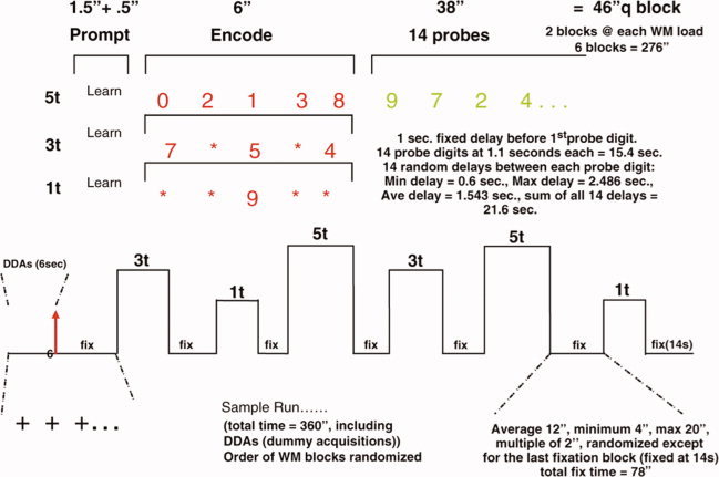
Each working memory set began with a learn prompt that lasted for 2 s and displayed the word “Learn,” followed by an encoding epoch that consisted of the simultaneous presentation of a set of targets (single‐digit numbers in red font) that lasted for 6 s. This was followed by a brief 1‐s delay followed by a 38‐s‐duration recognition epoch. Participants were then presented with a single digit in green font during this phase for 1.1 s, where half the digits are targets (digits from the encoding epoch) and the other half are foils. There was a random delay between each probe digit that ranged from a minimum of 0.6 s to a maximum delay of 2.5 s. In the fixation baseline epoch, a fixation cross appeared on the screen for a randomized duration that ranged from a minimum of 4 s to a maximum of 20 s. Prior to scanning, subjects were given instructions and practiced the task until they were comfortable. Only subjects performing to an accuracy criterion of 70% correct or better at each working memory load in a task run continued scanning. [Color figure can be viewed in the online issue, which is available at www.interscience.wiley.com.]

The participants studied at the four MCIC sites responded using the thumbs of each hand with the designated target thumb randomly assigned to the right or left hand. Participants studied at the fBIRN sites (all sites) utilized the index and middle fingers of the right hand to indicate targets and foils, respectively. Each subject was scanned while performing three runs of the SIRP paradigm. They were instructed to respond as quickly and accurately as possible and were given a bonus of 5 cents for each correct response. This bonus was provided after completion of the task, mailed to the participant a few weeks later, and was included to ameliorate motivational deficits. For Site 12 (total of 30 participants), reaction time data were not reported due to technical problems recording the timing of the button press.

Imaging Parameters

For all sites, pulse sequence parameters were mostly identical (orientation: AC‐PC line, number of slices: 27, slice thickness = 4 mm, 1 mm gap, TR = 2,000 ms, TE = 30 ms (3 T and 4 T)/40 ms (1.5 T), FOV = 22 cm, matrix 64 × 64, flip‐angle = 90°, voxel dimensions = 3.4375 × 3.4375 × 4 mm³). Site 3 utilized a spiral echo sequence while all other sites employed a single‐shot EPI sequence (Table II).

Table II.

Six sites used as part of this multisite analysisa

Site number	Institution	Patients	Controls	Scanner	Field strength	Sequence
3	Duke/UNC	11	17	GE Nvi Lx	4.0 T	Spiral
5	Brigham and Women's	5	5	GE	3.0 T	EPI
6	Mass. General Hospital	27	25	Siemens Trio	3.0 T	EPI
10	University of New Mexico	29	31	Siemens Sonata	1.5 T	EPI
12	University of Iowa	12	18	Siemens Trio	3.0 T	EPI
13	University of Minnesota	31	34	Siemens Trio	3.0 T	EPI

^aAll six sites consisted of a single 1.5 T and 4 T scanner along with five 3 T scanners.

Data Analysis: Preprocessing

Datasets were preprocessed using the software package SPM5 (http://www.fil.ion.ucl.ac.uk/spm/). Images were realigned using INRIalign—a motion correction algorithm unbiased by local signal changes (Freire and Mangin,2001; Freire et al.,2002). A slice‐timing correction was performed on the fMRI data after realignment to account for possible errors related to the temporal variability in the acquisition of the fMRI datasets. Data were spatially normalized (Ashburner and Friston,1999) into the standard Montreal Neurological Institute space using an SPM5 echo‐planar imaging (EPI) template and then spatially smoothed with a 9 × 9 × 9 mm³ full width at half‐maximum Gaussian kernel. The data (originally collected at 3.4 × 3.4 × 4 mm³) was slightly subsampled to 3 × 3 × 3 mm³ (during normalization) resulting in 53 × 63 × 46 voxels.

Data Analysis: Independent Component Analysis

A group spatial ICA was performed using the infomax algorithm (Bell and Sejnowski,1995) within the GIFT toolbox (http://icatb.sourceforge.net). The optimal number that ICA used to split the fMRI datasets into a final set of spatially independent functional networks was first determined using a modified minimum description length algorithm (Li et al.,2007), which was found to be 26. Since ICA with infomax is a stochastic process, the end results are not always identical. To remedy this, we utilized ICASSO (Himberg et al.,2004), originally applicable to single subjects only, recently implemented for group‐level analyses in the GIFT toolbox. ICASSO is an optimization algorithm that repeats an ICA analysis multiple times and finds the degree to which these components vary after each run. It then takes the centroid of these results and outputs a final set of components in addition to providing a measure of their consistency between different ICA analysis runs. For our purposes, we specified ICASSO to rerun ICA for 20 iterations.

The resulting output is an independent functional spatial map (referred to as a component) and a single ICA timecourse for every subject and session of fMRI scanning. In other words, for our subject pool of 245 participants, we acquired 19,110 (245 participants × 3 sessions × 26 components = 19,110) independent functional spatial maps along with their associated ICA timecourse. It is important to note that group ICA is performed on all the subjects at once and significant between‐group differences are determined by a second level analysis of the ICA results. It has been shown in previous studies that performing ICA on all subjects does not significantly detract or alter the results in comparison to an ICA analysis that is performed on each individual group separately (Calhoun et al.,2007, 2008, 2009). The benefit of applying ICA to all subjects avoids the problem of matching particular components from one group of subjects to another group, as ICA does not rank components in any specific order. By pooling across groups, the components are then comparable (e.g., Component 5 for Subject 1 will represent the same Component 5 for Subject 2 and so forth), for all subjects within the group ICA analysis.

Since the units that result from an ICA analysis are arbitrary, they need to be calibrated to reflect meaningful signal change. In this article, the ICA timecourses and spatial maps are calibrated using z‐scores (Beckmann et al.,2005). Every voxel within a component spatial map contains a z‐score, with regions that contain high z‐scores reflecting a greater contribution to the associated timecourse. Once the group ICA is performed, the spatial maps are averaged together across the three scan sessions. This averaging is performed within their respective components, resulting in 26 averaged component maps for each subject. These averaged spatial maps undergo a one‐sample t‐test for each component and are thresholded at an FDR‐corrected P‐threshold (P < 1 × 10⁻¹³) to determine their associated regions. As mentioned earlier, the spatial maps generated by ICA can also be thought of as functional connectivity maps, since their regions of activation share a single ICA timecourse. The degree of this relationship is reflected in the magnitude of the z‐scores. The voxel that has the greatest z‐score is considered to represent the idealized ICA timecourse, which has also been normalized using z‐scores. It is important to note that overlapping brain regions between independent spatial component maps are not uncommon and represents voxels that have a mixture of different timecourses.

To determine the relationship between the independent components and the experimental paradigm, a regression was performed on the ICA timecourses with the GLM design matrix. This allowed us to determine to what degree a given component is modulated by the different experimental phases (encode/probe: 1L, 3L, 5L). We can then test the resulting regression parameters to determine significant group differences. The regression results in a set of beta weights for every experimental regressor associated with the GLM design matrix. Every subject and their associated components are regressed, and thus each component contains the same number of beta weights as the number of regressors from the design matrix. The beta weights represent the degree to which the component was modulated by the task relative to the fixation baseline. A high beta weight then represents a large task‐related modulation for a given regressor within that component. This relationship is directly analogous to the GLM fit that is typically performed on neuroimaging studies of fMRI data (Fig. 2).

Figure 2.

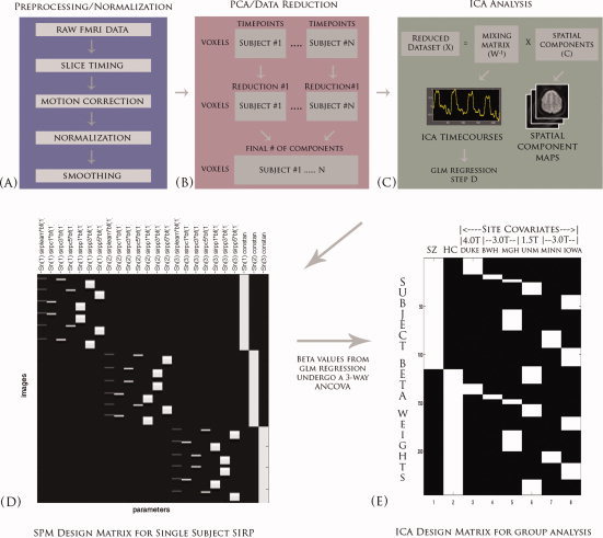
An overview of the ICA analyses. (A) Data was first preprocessed using SPM5 from the raw fMRI datasets. (B) After preprocessing, datasets are reduced using PCA across the time dimension to the parameter specified during the analysis. These datasets are further concatenated across time and reduced to a final number of dimensions, which is equal to the final number of components. (C) ICA splits this reduced dataset (X) into a mixing matrix (W‐1) that represents the ICA timecourses and a set of associated spatial components (C). (D) The ICA timecourses undergo a regression with the SPM design matrix to create a set of betas that will be used to determine task‐relevance and group differences. (E) The three‐way repeated measures ANCOVA is applied to our betas.

Component Selection

The ICA components of interest were selected in two stages. The first stage was to correlate each ICA component spatial map with prior probabilistic maps of white matter and cerebral spinal fluid (CSF) within a standardized brain space provided by the MNI templates in SPM5. One of the strengths of ICA is its ability to find noise‐related components that represent head motion, ventricle activity, eyeball movement, and other signal artifacts (McKeown et al.,2003). This approach has been utilized in previous studies of fMRI with ICA (Jafri et al.,2008; Stevens et al.,2007). If the spatial correlation for white matter was greater than r ² = 0.02 or r ² = 0.05 for CSF, then the component was considered to be artifactual and discarded.

From these remaining components, the second stage consisted of taking our β‐weights (generated from the regression of the GLM design matrix with the ICA timecourses) and inserting them into a three‐way repeated‐measures analysis of variance with covariates (ANCOVA). The β‐weights were averaged across sessions before inserting them into our ANCOVA. Our within‐subject factors were phase (P) and load (L), where phase contained two levels (encode and probe) and load contained three levels (low, medium, and high). Our dependent factor was group (G), which contained patients with schizophrenia and controls, and our covariates were site and accuracy. This type of analysis allowed us to account for potential site differences and to look at potentially significant interactions between various aspects of the WM task. Our criteria for determining interesting components were limited to significant group interactions with phase, load, or both at P < 0.05. We performed this ANCOVA twice, once with site as a single covariate and again using both site and accuracy. Depending on the type of interactions that existed, further analysis was performed to determine the source of this significance. For example, if there was a load by group interaction, a one‐way ANCOVA was performed to determine the effect each load had on that interaction.

Event‐related averages were also calculated to depict the shape of the ICA timecourse for each phase and load averaged across patients and controls separately. The event‐related averages show the direction of the ICA timecourse relative to the task and are normalized to start at zero during the onset of the learn phase. The window of time to depict the beginning of the learn phase to the end of the fixation phase was 26 TRs or 52 s.

RESULTS

Behavioral Findings

Patients and controls that performed lower than 75% accuracy during Probe 1, 70% for Probe 3, and 70% for Probe 5 were considered nonperformers and removed from the analysis. A total of 21 subjects were removed due to this threshold (15 patients/6 controls). Though average accuracy was high, even for patients during the highest WM load (93.7%), patients generally performed worse than controls across all WM loads, and these differences were found to be significant (Table III). Furthermore, reaction times were significantly different as well across WM loads, where patients were generally slower than controls in response to the presentation of WM items. Since the fBIRN and MCIC collaborations utilized a different motor response to the experimental stimuli, we performed a MANOVA to assess whether this affected the resulting accuracy or reaction times. We found that this interaction was not significant across all WM loads for both accuracy and reaction times when accounting for group differences. Tests of linearity were also performed for accuracy and reaction time as well as the averaged β‐weights (Table IV). It was found that there was a strong linear effect for both reaction time and accuracy when either accounting for group or collapsing across groups. A significant quadratic effect was seen for reaction time when collapsing across both groups.

Table III.

Two‐way MANOVA for site (S = fBIRN and MCIC) and group (G = patients and controls)

Reaction time	df	G × S (interaction)	G (interaction)	Mean/SE (HC)	Mean/SE (PZ)
R1	1	(F = 0.474, P = 0.492)	(F = 23.7, P < 0.001)	574.39/9.06	638.09/5.45
R2	1	(F = 0.089, P = 0.766)	(F = 40.9, P < 0.001)	659.62/10.3	754.97/10.8
R3	1	(F = 0.217, P = 0.642)	(F = 40.2, P < 0.001)	722.66/9.06	832.42/12.5
Accuracy	df	G × S (interaction)	G (interaction)	Mean/SE (HC)	Mean/SE (PZ)
A1	1	(F = 0.210, P = 0.647)	(F = 6.35, P = 0.012)	98.4/0.348	97.2/0.363
A2	1	(F = 0.184, P = 0.669)	(F = 13.2, P < 0.001)	97.9/0.432	95.6/0.451
A3	1	(F = 0.506, P = 0.478)	(F = 27.6, P < 0.001)	97.2/0.461	93.7/0.481

R1, R2, and R3 refer to reaction times for low, medium, and high loads, respectively. A1, A2, and A3 refer to the percentage of correct responses during the probe phase for low, medium, and high loads, respectively. No S × G interactions were found for either accuracy or reaction time. Significant differences were found between patients and controls across all WM loads.

Table IV.

Tests of linearity for reaction time, accuracy, and averaged beta‐weights

Behavior	df	Linear (RT)	Quadratic (RT)	Linear (RT × G)	Quadratic (RT × G)
RT	1	(F = 1,351, P < 0.001)	(F = 42.4, P < 0.001)	(F = 24.5, P < 0.001)	(F = 3.41, P = 0.066)
ACC	1	(F = 75.9, P < 0.001)	(F = 0.437, P = 0.509)	(F = 16.8, P < 0.001)	(F = 0.057, P = 0.811)
Beta values	df	Linear (L)	Quadratic (L)	Linear (L × P)	Quadratic (L × P)
C4	1	(F = 15.0, P < 0.001)	(F = 0.464, P = 0.497)	(F = 7.83, P = 0.006)	(F = 6.75, P = 0.010)
C15	1	(F = 2.59, P = 0.109)	(F = 7.46, P = 0.007)	(F = 1.62, P = 0.205)	(F = 0.529, P = 0.468)
C18	1	(F = 82.1, P < 0.001)	(F = 2.39, P = 0.123)	(F = 13.2, P < 0.001)	(F = 7.25, P = 0.008)
C20	1	(F = 2.84, P = 0.093)	(F = 6.84, P = 0.010)	(F = 16.2, P < 0.001)	(F = 0.859, P = 0.355)
C23	1	(F = 267, P < 0.001)	(F = 33.4, P < 0.001)	(F = 22.1, P < 0.001)	(F = 9.24, P = 0.003)
C24	1	(F = 182, P < 0.001)	(F = 0.192, P = 0.662)	(F = 14.5, P < 0.001)	(F = 1.72, P = 0.192)

G = group, RT = reaction time, ACC = percent accuracy, P = phase, L = load.

Discriminative Independent Components

Six components were identified that passed our selection criteria (Components C4, C15, C18, C20, C23, and C24). As mentioned before, this consisted of removing components that represented noise or artifactual activations, followed by a three‐way repeated measures ANCOVA with an F‐threshold of P < 0.05 for any group by load (G × L) or group by phase (G × P) interactions. Components that passed this threshold were subjected to an additional one‐way ANCOVA for further statistical inferences. Statistical results did not vary significantly when covarying for site or site and accuracy, except for C18 and C24, where the relevant interactions no longer showed significance when covaried for both site and accuracy (Table V). Our results from running ICASSO at the group level in GIFT showed that only C25 and C26 showed some spatial variability between each iteration of the ICA analysis, though these components were not found to show significant group differences nor overlap with any other component (Fig. 3). Selected brain slices and their associated event‐related averages are represented as either positively modulated (see Fig. 4) or negatively modulated (see Fig. 5) with the task, which refers to the general direction of the ICA timecourse across each phase. The event‐related averages for almost all of the components showed a peak amplitude around 8 s past the onset of the learn phase, which gradually shifted toward baseline by the end of the fixation phase. Mean β‐weights including error bars were plotted to visualize trends associated with increasing WM loads for both patients and controls during the encode/probe phases (Fig. 6).

Table V.

Results of three‐way repeated measures ANCOVA and one‐way univariate ANCOVAS

Group × phase (G × P) interactions (EN: encode; PR: probe)
Comps	df	G × P (site)	Controls (mean/SE)	Patients (mean/SE)	G × P (site + accuracy)	Controls (mean/SE)	Patients (mean/SE)
4	1	(F = 16.456, P < 0.0001)			(F = 14.331, P < 0.0001)
	1	EN: (F = 3.116, P = 0.079)	0.460/0.051	0.329/0.054	EN: (F = 2.312, P = 0.130)	0.452/0.052	0.336/0.055
	1	PR: (F = 3.940, P = 0.048)	0.289/0.040	0.406/0.043	PR: (F = 4.048, P = 0.045)	0.286/0.041	0.408/0.044
15	1	(F = 5.414, P = 0.021)			(F = 4.524, P = 0.034)
	1	EN: (F = 0.055, P = 0.814)	−0.218/0.042	−0.232/0.045	EN: (F = 0.438, P = 0.509)	−0.203/0.043	−0.345/0.046
	1	PR: (F = 6.183, P = 0.014)	−0.513/0.034	−0.390/0.036	PR: (F = 3.070, P = 0.081)	−0.494/0.034	−0.406/0.036
20	1	(F = 5.538, P = 0.019)			(F = 5.681, P = 0.018)
	1	EN: (F = 0.173, P = 0.678)	−0.253/0.043	−0.279/0.047	EN: (F = 0.432, P = 0.512)	−0.244/0.044	−0.287/0.047
	1	PR: (F = 5.999, P = 0.015)	−0.420/0.033	−0.301/0.036	PR: (F = 4.734, P = 0.031)	−0.415/0.034	−0.306/0.036
23	1	(F = 11.567, P = 0.001)			(F = 8.176, P = 0.005)
	1	EN: (F = 1.846, P = 0.176)	0.882/0.057	0.768/0.061	EN: (F = 1.042, P = 0.308)	0.868/0.058	0.780/0.062
	1	PR: (F = 4.579, P = 0.033)	0.582/0.039	0.703/0.041	PR: (F = 3.826, P = 0.052)	0.585/0.039	0.700/0.042
24	1	(F = 4.231, P = 0.041)			(F = 2.361, P = 0.126)
	1	EN: (F = 2.047, P = 0.154)	−0.475/0.052	−0.584/0.055	EN: (F = 2.888, P = 0.091)	−0.462/0.053	−0.595/0.056
	1	PR: (F = 12.548, P < 0.001)	−0.273/0.045	−0.514/0.048	PR: (F = 11.994, P < 0.001)	−0.277/0.046	−0.511/0.048

Group × load interactions (L1: low, L2: medium, L3: high | WM loads)
Comps	df	G × L (site)	Controls (mean/SE)	Patients (mean/SE)	G × L (site + accuracy)	Controls (mean/SE)	Patients (mean/SE)
18	2	(F = 3.288, P = 0.039)			(F = 2.214, P = 0.112)
	1	L1: (F = 1.303, P = 0.255)	−0.249/0.042	−0.179/0.045	L1: (F = 0.779, P = 0.378)	−0.242/0.043	−0.186/0.045
	1	L2: (F = 0.063, P = 0.801)	−0.311/0.041	−0.326/0.043	L2: (F = 0.078, P = 0.780)	−0.310/0.041	−0.327/0.044
	1	L3: (F = 6.170, P = 0.014)	−0.603/0.046	−0.436/0.049	L3: (F = 3.911, P = 0.049)	−0.586/0.046	−0.450/0.049
23	2	(F = 4.045, P = 0.019)			(F = 3.618, P = 0.028)
	1	L1: (F = 1.564, P = 0.212)	0.501/0.043	0.422/0.046	L1: (F = 1.614, P = 0.205)	0.504/0.044	0.420/0.047
	1	L2: (F = 2.378, P = 0.124)	0.565/0.049	0.677/0.053	L2: (F = 2.245, P = 0.135)	0.565/0.050	0.677/0.054
	1	L3: (F = 0.053, P = 0.818)	1.129/0.061	1.108/0.065	L3: (F = 0.015, P = 0.904)	1.112/0.062	1.123/0.066

G = group, P = phase, L = load, EN = mean(L1 + L2 + L3) encode, PR = mean(L1 + L2 + L3) probe, L1 = low load, L2 = medium load, L3 = high load.

Figure 3.

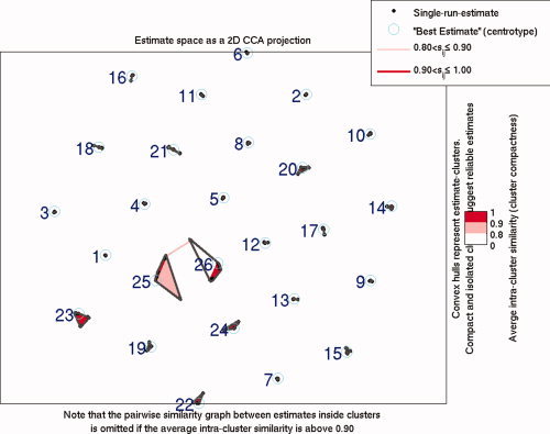
Clustering results from the group‐level ICASSO implemented in the GIFT toolbox. The greatest spatial variability can be seen in C25 and C26. [Color figure can be viewed in the online issue, which is available at www.interscience.wiley.com.]

Figure 4.

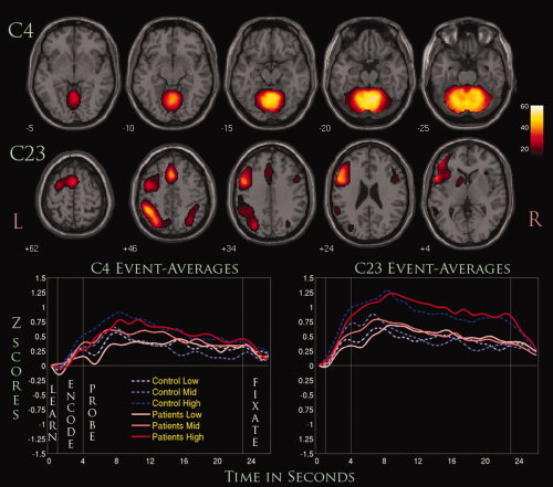
Two positively modulated components (C4 and C23). Displayed are selected slices from each component thresholded at (P < 1.0 × 10⁻¹³, FDR) along with their event‐related averages.

Figure 5.

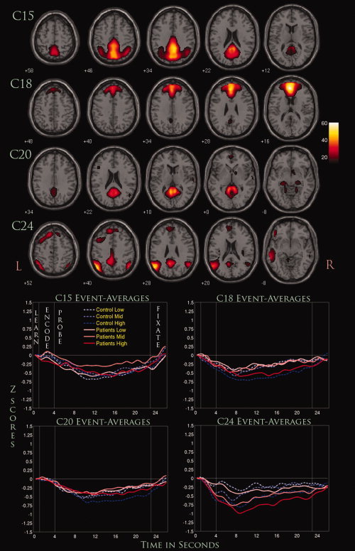
Four negatively modulated components (C15, C18, C20, and C24). Displayed are selected slices from each component thresholded at (P < 1.0 × 10⁻¹³, FDR) along with their event‐related averages.

Figure 6.

Averaged encode and probe β‐weights with standard error bars for each WM load and group.

Positively Task‐Modulated Networks

C4 consisted primarily of regions within the cerebellum with wide activations seen in the declive and culmen (Table VI). The three‐way repeated measures ANCOVA showed a significant G × P interaction between the encode and probe phase, suggesting that it was modulated differently for patients and controls. The one‐way follow‐up ANCOVA showed that this interaction seemed to stem from both phases when covaried for site only, where the marginal means for controls were greater than those for patients. When covarying for both site and accuracy, the interaction was seen to stem primarily from the probe phase. Linear effects were seen across load (L) for this component and when phase differences were taken into account (L × P) (see Fig. 4). Quadratic effects were also shown to be significant as well, but only for L × P interactions.

Table VI.

The top five brain regions (max t‐values) based on random effects one sample t‐test analysis in SPM

	Brodmann areas	R/L (cm3)	R/L (max‐t, MNI coordinates)
Comp 4
Declive		12.9/12.6	53.8 (−9,−59,−12)/51.7 (27,−59,−22)
Culmen		12.7/13.0	53.0 (−12,−56,−15)/50.8 (0,−56,−15)
Uvula		1.4/1.9	48.6 (0,−68,−27)/46.4 (33,−62,−25)
Pyramis		2.0/2.4	47.4 (0,−65,−24)/43.9 (3,−65,−24)
Dentate gyrus	19	6.2/5.9	45.3 (0,−76,−14)/44.0 (33,−54,−28)
Comp 15
Cingulate gyrus	31, 23, 24	10.7/8.5	48.4 (−3,−45,33)/43.7 (3,−42,33)
Precuneus	31, 7, 23, 19, 39, 18	27.2/25.9	47.9 (−3,−48,33)/42.8 (3,−48,30)
Cuneus	7, 19, 18	2.9/3.3	41.1 (0,−65,31)/41.5 (6,−68,31)
Posterior cingulate	23, 31, 30, 29	4.3/4.3	41.0 (−6,−45,24)/40.1 (6,−48,25)
Paracentral lobule	31, 5, 6	3.3/2.6	37.1 (0,−30,43)/36.6 (3,−30,43)
Comp 18
Anterior cingulate	32, 24, 10, 25, 33, 9	9.1/8.9	57.6 (−3,44,3)/61.2 (3,47,6)
Medial frontal gyrus	10, 9, 32, 6, 8	11.3/12.7	55.4 (−3,47,11)/60.2 (3,50,6)
Superior frontal gyrus	9, 10, 8	12.6/10.8	44.7 (−3,54,22)/42.8 (3,56,22)
Corpus callosum		3.5/3.6	39.0 (−3,32,4)/39.4 (3,32,4)
Cingulate gyrus	32, 9, 24, 31	1.9/2.1	37.6 (−3,36,26)/39.5 (3,36,26)
Comp 20
Posterior cingulate	29, 23, 30, 31	6.5/7.2	44.4 (−9,−49,8)/46.2 (6,−46,8)
Parahippocampal gyrus	30, 28, 36, 35, 19, 27, 37, 34	5.5/4.3	41.7 (−9,−46,5)/42.3 (9,−46,5)
Lateral globus pallidus		3.9/1.6	35.7 (−6,−43,10)/38.6 (3,−40,8)
Culmen		2.8/2.9	33.6 (−9,−47,2)/37.1 (9,−47,2)
Lingual gyrus	18, 19	1.5/1.4	34.8 (−12,−52,5)/31.9 (12,−52,5)
Comp 23
Inferior parietal lobule	40, 7, 39	5.2/11.7	24.2 (−33,−59,47)/45.6 (42,−44,46)
Inferior frontal gyrus	47, 9, 44, 45, 46, 6, 10, 13, 11	3.7/19.2	20.6 (−36,23,−4)/42.3 (50,13,21)
Medial frontal gyrus	8, 6, 32, 9	2.5/5.2	40.9 (−3,17,46)/41.7 (3,20,43)
Superior frontal gyrus	6, 8, 10	2.8/6.9	41.6 (0,14,49)/39.0 (3,14,49)
Cingulate gyrus	32, 24, 9	2.0/4.0	36.8 (−3,20,40)/40.7 (3,22,40)
Comp 24
Angular gyrus	39	1.3/2.3	32.3 (−50,−59,36)/51.4 (50,−62,36)
Supramarginal gyrus	40	3.2/4.4	31.3 (−50,−57,33)/50.8 (53,−60,33)
Inferior parietal lobule	39, 40, 7	3.4/7.0	32.6 (−50,−59,39)/49.6 (50,−62,39)
Middle temporal gyrus	39, 21, 19, 22	1.3/13.9	24.9 (−50,−60,28)/46.4 (50,−63,28)
Superior temporal gyrus	39, 22, 21, 13, 41	1.2/9.0	27.5 (−53,−57,28)/45.7 (53,−60,28)

A Talairach labeling system was used to determine regions of significance at a threshold of (P < 1.0 × 10⁻¹³, FDR).

The regions C23 engaged were heavily lateralized to the left hemisphere, recruiting regions such as the DLPFC, IPL, and cingulate gyrus. This component was also the only one to show significant interactions for both G × P and G × L interactions. The probe phase, when averaged across loads, seemed to be responsible for the significant G × P interaction, where patients were greater than controls in their averaged beta‐weights. For the G × L interactions, no individual load condition seemed to be responsible for its significance, suggesting that the combination of load differences played a significant role. Furthermore, controls were greater than patients in their averaged beta‐weights for the low and high load conditions, while patients were greater than controls for the medium WM load condition. Linearity tests showed significant linear and quadratic effects for all L and L × P interaction.

Negatively Task‐Modulated Networks

C15 represented regions primarily within the posterior cingulate, precuneus, and cuneus. There was a significant G × P interaction with greater differences seen in the probe phase. Covarying for both site and accuracy did not significantly alter the results. The marginal means were negative for both groups, suggesting a negative task‐associated modulation of the component timecourse. In this regard, controls were more negative than patients with the lowest amplitude for both groups occurring around 12 s after the onset of the learn phase. A significant quadratic effect was seen only for the load‐averaged interaction.

C18 showed widespread activation centered on the medial frontal gyrus, bordering regions of the superior frontal gyrus. G × L interactions were significant when only covarying for site, suggesting that accuracy played a significant role in generating group differences. Controls were more negative than patients across the low and high WM loads, while patients were slightly more negative in the medium WM load. A further ANCOVA showed that the significance for this interaction was mostly due to the highest WM load. Significant linear effects were seen for both L and L × P interactions, but no significant quadratic effects were found.

C20 showed significant activations primarily in the posterior cingulate and parahippocampal gyrus along with some subcortical regions such as the lateral globus pallidus and culmen. A significant G × P interaction was seen when covarying for just site or site along with accuracy. This significance was primarily driven by the probe phase, where the marginal means were more negative for controls than patients. Linearity tests showed a significant quadratic effect occurring with L, but along with a significant linear effect for L × P interactions.

C24 engaged a variety of regions, including the angular and supramarginal gyrus, IPL, and superior and middle temporal gyrus. G × P interactions were significant only when covaried for site, where the significance was driven almost entirely by the probe phase. The marginal means for patients were considerably more negative than controls where the event‐related averages show a considerably greater decrease across all WM loads. Linearity tests showed a significant linear effect for both L and L × P interactions, but no quadratic effects were found to be significant.

DISCUSSION

Using ICA, we were able to filter out noise/artifactual components of the fMRI signal to identify the anatomical components of putative brain networks involved in WM based on their synchronous activation. We were also able to examine differences in the functioning of these networks in patients with schizophrenia compared to healthy controls. Our results confirmed our hypotheses, as we found strong differences in C23, a network of WM regions (DLPFC and IPL) and C4 (cerebellum), engaging motor‐related regions. Significant differences were also seen in networks (C15, C18, C20, and C24) spanning brain regions known to be associated with the DMN. The number of networks shown to have significant between‐group differences suggests that the cognitive pathophysiology of schizophrenia is widespread. Furthermore, this dysfunction extends to the DMN, and the number of networks that span its associated regions provide some support for the idea that this network is not singular, but a conglomeration of multiple subnetworks that work in conjunction with one another (Uddin et al.,2009).

In regard to the manipulation and storage of WM items, C23 is considerably significant, since it engages both the DLPFC and IPL. Studies have shown that the DLPFC is tightly linked to the “on‐line” maintenance of WM items and that dysfunction in this area is prominent in patients with schizophrenia (Goldman‐Rakic,1994) and their first degree relatives (Seidman et al.,2006). The IPL has been known to be intricately connected to the DLPFC (Cole and Schneider,2007) and several studies have focused on the relationship between these two regions in modulating WM processes (Barch and Csernansky,2007; Calhoun et al.,2006; Kim et al.,2003). Other regions were implicated as well, including the medial frontal gyrus and some portion of the anterior cingulate. These regions are known to be implicated in high‐level executive functions and decision‐related processes (Talati and Hirsch,2005) and might assist in the storage and retrieval of WM items. The network of regions associated with C4 was predominantly cerebellar. The cerebellum is known to assist in the smooth coordination of complex motor‐activity, and its activation could be a result of the button presses associated with the retrieval and recognition of WM items. More subtle differences in this brain region have been posited (Schlosser et al.,2003), where patients with schizophrenia showed reduced connectivity between the prefrontal and cerebellar pathways during a WM task. This finding adds some support to the notion that patients with schizophrenia might suffer from a dysfunction in the connectivity of these two networks during WM processes.

Our three‐way ANCOVA showed that C23 was affected by both G × P and G × L interactions, but not the G × L × P interactions. The lack of significance for the G × L × P could suggest that differences in patients with schizophrenia, which stem from the encoding and probing of WM items, might not be significantly related to the modulation of WM processes as the number of items increases. The G × P interactions were driven almost entirely by the probe phase, which was also the case for any component that had significant interactions of this sort. Whether this is partially due to the fact that the probe phase was considerably longer is difficult to tell. However, the DLPFC and IPL have been consistently shown to be linked to WM dysfunction in schizophrenia, and our results suggest that this relationship may be stronger during the recognition and retrieval of WM items, which is associated with the probe phase of the paradigm. For the G × L interaction, the medium WM load was found to be the most significant, counter to the idea that higher WM loads would better extract these differences. However, our findings are consistent with a recent schizophrenia WM study (Potkin et al.,2009), which utilized data from the same fBIRN collaboration and found that the medium WM load was most responsible for significant between‐group differences in the DLPFC. Their conclusion was that these differences are more strongly related to the “inefficiency” of this brain region that might not be directly caused by increases in WM load.

A significant number of fMRI studies in schizophrenia have now focused on the DMN and its potential dysfunction in schizophrenia (Calhoun et al.,2007; Garrity et al.,2007; Pomarol‐Clotet et al.,2008; Whitfield‐Gabrieli et al.,2009). Our current results support this claim, as the four negatively modulated networks we found were composed entirely of regions hypothesized to be engaged in the DMN. These included the medial prefrontal cortex (found in C18 and C24), ventral anterior cingulate (C18), parahippocampus (C20), posterior cingulate (C15, C18, C20, and C24), precuneus (C15) and some regions of the lateral parietal cortex (C24) (Buckner et al.,2008). The fact that these networks were not conglomerated into a single network using ICA suggests that the DMN might consist of multiple networks that work in conjunction with one another to perform complex tasks such as introspection, goal‐planning, and general nontask‐oriented activities. Furthermore, these four networks have a single common region in the PCC, which Buckner et al. (2008) suggested could modulate different subsystems within the DMN. However, further analyses would be needed to determine if these networks have specific connectivity relationships with one another, which our current study cannot provide.

Our three‐way ANCOVA of the four networks associated with the DMN showed some interesting trends that may pertain to the dysfunction of WM processes in schizophrenia. The DMN, more than other temporally coherent resting state networks, has been shown to share a continuous competitive relationship with networks necessary for task completion (Broyd et al., 2008). Further, the degree of deactivation that occurs in this network is influenced by task type (Tomasi et al.,2006), task load (McKiernan et al.,2003), and schizophrenia diagnosis (Harrison et al.,2007). Load sensitivity in the current WM study was evident for C18, where increasing WM load was associated with increased deactivation of the component timecourse. For C18, controls deactivated more than patients across the low and high WM loads for both phases, while patients deactivated slightly more than controls for the medium WM load. However, when covarying for accuracy, G × L interactions were no longer significant, suggesting that significant between‐group differences associated with WM load might be task‐dependent. For C24, an interesting trend was seen where patients were consistently deactivated more than controls across all WM loads for both phases. However, G × P interactions were only found to be significant for this network, and this significance no longer existed when covarying for accuracy. In this context, C18 and C24 seem to represent differences associated to some degree with poor WM performance, which has been shown to be a prominent marker for this illness. It can be hypothesized then that these two networks might play a significant role in WM processes, and a dysfunction in the normal deactivation of these networks could impair such processes.

As for C15 and C20, G × P interactions remained significant when covarying for accuracy, indicating that these networks may represent a more stable functional marker of schizophrenia. Supporting evidence for this comes from a recent study using an identical ICA analysis approach on datasets from the same fBIRN collaboration, which found highly significant differences in patients with schizophrenia in an ICA network nearly identical to C15 during the completion of an auditory oddball paradigm (Kim et al.,2009). It is also worth noting that these G × P interactions reflect an interesting reversal of brain deactivation between patients and controls during the encode and probe phases. Patients show a greater deactivation for both networks during encoding of WM items, but this is reversed during the probe phase, where controls show a significantly greater deactivation. This trend was also seen in C4, a positively modulated network that engaged primarily the cerebellum. This phenomenon might be related to an inefficiency in the modulation of task‐oriented networks that need to be activated sufficiently for proper WM processes to occur. Recent studies have suggested that a dysfunction in the intricate interplay between task‐positive and task‐negative networks might be associated with schizophrenia (Jafri et al.,2008), and our results provide some support for those ideas. These inefficiencies might be found in other modalities as well (i.e., MEG, EEG), and future work in this direction could further elucidate the pathophsyiology of schizophrenia (Calhoun et al.,2009).

There are several limitations to the present study. Schizophrenia is a heterogeneous disorder, and biomarkers that identify subgroups or regions with high inter‐subject morphologic or functional variability may be obscured by group averaging (Manoach,2003). Though we attempted to account for the effect of site by including it as a covariate in our ANCOVA models, it is still possible that this factor increased the variability of the data and obscured findings of interest. Another concern is the possibility that patients with schizophrenia may be characterized by reduced attentional control or reduced motivation, and that these attentional or motivational differences may have resulted in the observed deficits in WM performance and functional activation. We attempted to control for this concern by motivating all participants with a monetary reward for each correct trial. Nonetheless, it is possible that remaining differences in attention or motivation could have been responsible for some group differences noted. Intelligence measures were also different for the fBIRN and MCIC collaborations, utilizing the NART and WRAT measurements, respectively, and thus we omitted the reporting of these measurements. Finally, we normalized our datasets to an MNI template that might not be sensitive to volumetric differences found in patients with schizophrenia. An averaged brain template, reflective of our population, could allow for a more accurate assessment of the anatomical locations of these functional connectivity differences.

CONCLUSION

Using ICA we were able to discern functionally connected networks that extend our understanding of the interplay between various brain regions related to WM processing. We implemented ICASSO at the group level for the first time to find results that were averaged across twenty iterations of ICA. A robust statistical analysis of the task‐modulation parameters from our component timecourses was performed, resulting in the observation of six disease‐relevant networks. Two of these networks were hypothesized to be positively task‐modulated and include regions such as the DLPFC and cerebellum. The other four were thought to represent parts of the DMN that shared the PCC as a common brain region. To our knowledge, this is the largest WM analysis of ICA performed with a population of patients with schizophrenia and healthy controls. Our results show many of the same neurobiological markers found from previous WM studies to be implicated using a functional connectivity approach via ICA. We further extend these markers to suggest that the DLPFC is implicated in schizophrenia within a network that includes regions of the IPL and cingulate gyrus. Finally, we show that the DMN might exist across multiple subnetworks and that schizophrenia could be marked by a dysfunction that spans across them.

REFERENCES

- Andreasen NC, editor ( 1983): Scale for the Assessment of Negative Symptoms (SANS). Iowa City: University of Iowa. [Google Scholar]
- Andreasen NC, editor ( 1984): Scale for the Assessment of Positive Symptoms (SAPS). Iowa City: University of Iowa. [Google Scholar]
- Ashburner J, Friston KJ ( 1999): Nonlinear spatial normalization using basis functions. Hum Brain Mapp 7: 254– 266. [DOI] [PMC free article] [PubMed] [Google Scholar]
- Baddeley A ( 1976): The Psychology of Memory. New York: Basic Books. [Google Scholar]
- Baddeley A ( 1992): Working memory. Science 255: 556– 559. [DOI] [PubMed] [Google Scholar]
- Barch DM ( 2006): What can research on schizophrenia tell us about the cognitive neuroscience of working memory? Neuroscience 139: 73– 84. [DOI] [PubMed] [Google Scholar]
- Barch DM, Csernansky JG ( 2007): Abnormal parietal cortex activation during working memory in schizophrenia: Verbal phonological coding disturbances versus domain‐general executive dysfunction. Am J Psychiatry 164: 1090– 1098. [DOI] [PubMed] [Google Scholar]
- Beckmann CF, De Luca M, Devlin JT, Smith SM ( 2005): Investigations into resting‐state connectivity using Independent Component Analysis. Philos Trans R Soc Lond B Biol Sci 360: 1001– 1013. [DOI] [PMC free article] [PubMed] [Google Scholar]
- Bell AJ, Sejnowski TJ ( 1995): An information maximisation approach to blind separation and blind deconvolution. Neural Comput 7: 1129– 1159. [DOI] [PubMed] [Google Scholar]
- Bockholt HJ, Williams S, Scully M, Magnotta V, Gollub R, Lauriello J, Lim K, White T, Jung RE, Schulz SC, Andreasen N, Calhoun V ( 2008): The MIND Clinical Imaging Consortium as an application for novel comprehensive quality assurance procedures in a multi‐site heterogeneous clinical research study. Presented at the 14th Annual Meeting of the Organization for Human Brain Mapping, Melbourne, Australia, 15–19 June 2008.
- Broyd SJ, Demanuele C, Debener S, Helps SK, James CJ, Sonuga‐Barke EJ ( 2009): Default‐mode brain dysfunction in mental disorders: A systematic review. Neurosci Biobehav Rev 33: 279– 296. [DOI] [PubMed] [Google Scholar]
- Buckner RL, Andrews‐Hanna JR, Schacter DL ( 2008): The brain's default network: Anatomy, function, and relevance to disease. Ann N Y Acad Sci 1124: 1– 38. [DOI] [PubMed] [Google Scholar]
- Calhoun VD, Adali T, Pearlson GD, Pekar JJ ( 2001a): A method for making group inferences from functional MRI data using independent component analysis. Hum Brain Mapp 14: 140– 151. [DOI] [PMC free article] [PubMed] [Google Scholar]
- Calhoun VD, Adali T, Pearlson GD, Pekar JJ ( 2001b): Spatial and temporal independent component analysis of functional MRI data containing a pair of task‐related waveforms. Hum Brain Mapp 13: 43– 53. [DOI] [PMC free article] [PubMed] [Google Scholar]
- Calhoun VD, Adali T, Giuliani NR, Pekar JJ, Kiehl KA, Pearlson GD ( 2006): Method for multimodal analysis of independent source differences in schizophrenia: Combining gray matter structural and auditory oddball functional data. Hum Brain Mapp 27: 47– 62. [DOI] [PMC free article] [PubMed] [Google Scholar]
- Calhoun VD, Maciejewski PK, Pearlson GD, Kiehl KA ( 2007): Temporal lobe and “default” hemodynamic brain modes discriminate between schizophrenia and bipolar disorder. Hum Brain Mapp 29: 1265– 1275. [DOI] [PMC free article] [PubMed] [Google Scholar]
- Calhoun VD, Kiehl KA, Pearlson GD ( 2008): Modulation of temporally coherent brain networks estimated using ICA at rest and during cognitive tasks. Hum Brain Mapp 29: 828– 838. [DOI] [PMC free article] [PubMed] [Google Scholar]
- Calhoun VD, Liu J, Adali T ( 2009): A review of group ICA for fMRI data and ICA for joint inference of imaging, genetic, and ERP data. Neuroimage 45( 1 Suppl): S163– S172. [DOI] [PMC free article] [PubMed] [Google Scholar]
- Cannon TD, Keller MC ( 2006): Endophenotypes in the genetic analyses of mental disorders. Annu Rev Clin Psychol 2: 267– 290. [DOI] [PubMed] [Google Scholar]
- Cohen JD, Braver TS, O'Reilly RC ( 1996): A computational approach to prefrontal cortex, cognitive control and schizophrenia: Recent developments and current challenges. Philos Trans R Soc Lond B Biol Sci 351: 1515– 1527. [DOI] [PubMed] [Google Scholar]
- Cole MW, Schneider W ( 2007): The cognitive control network: Integrated cortical regions with dissociable functions. Neuroimage 37: 343– 360. [DOI] [PubMed] [Google Scholar]
- Damoiseaux JS, Rombouts SA, Barkhof F, Scheltens P, Stam CJ, Smith SM, Beckmann CF ( 2006): Consistent resting‐state networks across healthy subjects. Proc Natl Acad Sci USA 103: 13848– 13853. [DOI] [PMC free article] [PubMed] [Google Scholar]
- De Luca M, Beckmann CF, De Stefano N, Matthews PM, Smith SM ( 2006): fMRI resting state networks define distinct modes of long‐distance interactions in the human brain. Neuroimage 29: 1359– 1367. [DOI] [PubMed] [Google Scholar]
- Demirci O, Clark VP, Magnotta V, Andreasen NC, Lauriello J, Kiehl KA, Pearlson GD, Calhoun VD ( 2008): A review of challenges in the use of fMRI for disease classification/characterization and a projection pursuit application from multi‐site fMRI schizophrenia study. Brain Imaging Behav 2: 207– 226. [DOI] [PMC free article] [PubMed] [Google Scholar]
- First MB, Spitzer RL, Gibbon M, Williams JBW ( 1995): Structured clinical interview for DSM‐IV axis I disorders‐patient edition (SCID‐I/P, Version 2.0). New York: Biometrics Research Department, New York State Psychiatric Institute. [Google Scholar]
- Freire L, Mangin JF ( 2001): Motion correction algorithms may create spurious brain activations in the absence of subject motion. NeuroImage 14: 709– 722. [DOI] [PubMed] [Google Scholar]
- Freire L, Roche A, Mangin JF ( 2002): What is the best similarity measure for motion correction in fMRI time series? IEEE Trans Med Imaging 21: 470– 484. [DOI] [PubMed] [Google Scholar]
- Friston KJ ( 1999): Schizophrenia and the disconnection hypothesis. Acta Psychiatr Scand Suppl 395: 68– 79. [DOI] [PubMed] [Google Scholar]
- Garrity AG, Pearlson GD, McKiernan K, Lloyd D, Kiehl KA, Calhoun VD ( 2007): Aberrant “default mode” functional connectivity in schizophrenia. Am J Psychiatry 164: 450– 457. [DOI] [PubMed] [Google Scholar]
- Goldman‐Rakic PS ( 1991): Prefrontal cortical dysfuntion in schizophrenia: The relevance of working memory In: Carroll BJ, Barrett JE, editors. Psychopathology and the Brain. New York: Raven Press; pp 1– 23. [Google Scholar]
- Goldman‐Rakic PS ( 1994): Working memory dysfunction in schizophrenia. J Neuropsychiatry Clin Neurosci 6: 348– 357. [DOI] [PubMed] [Google Scholar]
- Harrison BJ, Yucel M, Pujol J, Pantelis C ( 2007): Task‐induced deactivation of midline cortical regions in schizophrenia assessed with fMRI. Schizophr Res 91( 1–3): 82– 86. [DOI] [PubMed] [Google Scholar]
- Himberg J, Hyvarinen A, Esposito F ( 2004): Validating the independent components of neuroimaging time series via clustering and visualization. Neuroimage 22: 1214– 1222. [DOI] [PubMed] [Google Scholar]
- Honey GD, Fletcher PC ( 2006): Investigating principles of human brain function underlying working memory: What insights from schizophrenia? Neuroscience 139: 59– 71. [DOI] [PubMed] [Google Scholar]
- Jafri MJ, Pearlson GD, Stevens M, Calhoun VD ( 2008): A method for functional network connectivity among spatially independent resting‐state components in schizophrenia. Neuroimage 39: 1666– 1681. [DOI] [PMC free article] [PubMed] [Google Scholar]
- Johnson MR, Morris NA, Astur RS, Calhoun VD, Mathalon DH, Kiehl KA, Pearlson GD ( 2006): A functional magnetic resonance imaging study of working memory abnormalities in schizophrenia. Biol Psychiatry 60: 11– 21. [DOI] [PubMed] [Google Scholar]
- Kim JJ, Kwon JS, Park HJ, Youn T, Kang DH, Kim MS, Lee DS, Lee MC ( 2003): Functional disconnection between the prefrontal and parietal cortices during working memory processing in schizophrenia: A [15(O)]H2O PET study. Am J Psychiatry 160: 919– 923. [DOI] [PubMed] [Google Scholar]
- Kim DI, Mathalon DH, Ford JM, Mannell M, Turner JA, Brown GG, Belger A, Gollub R, Lauriello J, Wible C, O'Leary D, Lim K, Toga A, Potkin SG, Birn F, Calhoun VD ( 2009): Auditory oddball deficits in schizophrenia: An independent component analysis of the fMRI multisite function BIRN study. Schizophr Bull 35: 67– 81. [DOI] [PMC free article] [PubMed] [Google Scholar]
- Li YO, Adali T, Calhoun VD ( 2007): Estimating the number of independent components for functional magnetic resonance imaging data. Hum Brain Mapp 28: 1251– 1266. [DOI] [PMC free article] [PubMed] [Google Scholar]
- Manoach DS ( 2003): Prefrontal cortex dysfunction during working memory performance in schizophrenia: Reconciling discrepant findings. Schizophr Res 60( 2/3): 285– 298. [DOI] [PubMed] [Google Scholar]
- Manoach DS, Schlaug G, Siewert B, Darby DG, Bly BM, Benfield A, Edelman RR, Warach S ( 1997): Prefrontal cortex fMRI signal changes are correlated with working memory load. Neuroreport 8: 545– 549. [DOI] [PubMed] [Google Scholar]
- Manoach DS, Press DZ, Thangaraj V, Searl MM, Goff DC, Halpern E, Saper CB, Warach S ( 1999): Schizophrenic subjects activate dorsolateral prefrontal cortex during a working memory task, as measured by fMRI. Biol Psychiatry 45: 1128– 1137. [DOI] [PubMed] [Google Scholar]
- Manoach DS, Greve DN, Lindgren KA, Dale AM ( 2003): Identifying regional activity associated with temporally separated components of working memory using event‐related functional MRI. Neuroimage 20: 1670– 1684. [DOI] [PubMed] [Google Scholar]
- McKeown MJ, Makeig S, Brown GG, Jung TP, Kindermann SS, Bell AJ, Sejnowski TJ ( 1998): Analysis of fMRI data by blind separation into independent spatial components. Hum Brain Mapp 6: 160– 188. [DOI] [PMC free article] [PubMed] [Google Scholar]
- McKeown MJ, Hansen LK, Sejnowsk TJ ( 2003): Independent component analysis of functional MRI: What is signal and what is noise? Curr Opin Neurobiol 13: 620– 629. [DOI] [PMC free article] [PubMed] [Google Scholar]
- McKiernan KA, Kaufman JN, Kucera‐Thompson J, Binder JR ( 2003): A parametric manipulation of factors affecting task‐induced deactivation in functional neuroimaging. J Cogn Neurosci 15: 394– 408. [DOI] [PubMed] [Google Scholar]
- Meda SA, Bhattarai M, Morris NA, Astur RS, Calhoun VD, Mathalon DH, Kiehl KA, Pearlson GD ( 2008): An fMRI study of working memory in first‐degree unaffected relatives of schizophrenia patients. Schizophr Res 104( 1–3): 85– 95. [DOI] [PMC free article] [PubMed] [Google Scholar]
- Meyer‐Lindenberg A, Poline JB, Kohn PD, Holt JL, Egan MF, Weinberger DR, Berman KF ( 2001): Evidence for abnormal cortical functional connectivity during working memory in schizophrenia. Am J Psychiatry 158: 1809– 1817. [DOI] [PubMed] [Google Scholar]
- Park S, Holzman PS, Goldman‐Rakic PS ( 1995): Spatial working memory deficits in the relatives of schizophrenic patients. Arch Gen Psychiatry 52: 821– 828. [DOI] [PubMed] [Google Scholar]
- Pomarol‐Clotet E, Salvador R, Sarro S, Gomar J, Vila F, Martinez A, Guerrero A, Ortiz‐Gil J, Sans‐Sansa B, Capdevila A, Cebamanos JM, McKenna PJ ( 2008): Failure to deactivate in the prefrontal cortex in schizophrenia: Dysfunction of the default mode network? Psychol Med 38: 1185– 1193. [DOI] [PubMed] [Google Scholar]
- Potkin SG, Ford JM ( 2009): Widespread cortical dysfunction in schizophrenia: The fBIRN imaging consortium. Schizophr Bull 35: 15– 18. [DOI] [PMC free article] [PubMed] [Google Scholar]
- Potkin SG, Turner J, Brown GG, McCarthy G, Greve DN, Glover GH, Manoach DS, Belger A, Diaz M, Wible CG, Ford JM, Mathalon DH, Gollub R, Lauriello J, O'Leary D, van Erp TG, Toga AW, Preda A, Lim KO; fBIRN ( 2009): Working memory and DLPFC inefficiency in schizophrenia: The FBIRN study. Schizophr Bull 35: 19– 31. [DOI] [PMC free article] [PubMed] [Google Scholar]
- Schlosser R, Gesierich T, Kaufmann B, Vucurevic G, Hunsche S, Gawehn J, Stoeter P ( 2003): Altered effective connectivity during working memory performance in schizophrenia: A study with fMRI and structural equation modeling. Neuroimage 19: 751– 763. [DOI] [PubMed] [Google Scholar]
- Seidman LJ, Thermenos HW, Poldrack RA, Peace NK, Koch JK, Faraone SV, Tsuang MT ( 2006): Altered brain activation in dorsolateral prefrontal cortex in adolescents and young adults at genetic risk for schizophrenia: An fMRI study of working memory. Schizophr Res 85( 1–3): 58– 72. [DOI] [PubMed] [Google Scholar]
- Sternberg S ( 1966): High‐speed scanning in human memory. Science 153: 652– 654. [DOI] [PubMed] [Google Scholar]
- Sternberg S ( 1969): Memory‐scanning: Mental processes revealed by reaction time experiments. Am Sci 57: 421– 457. [PubMed] [Google Scholar]
- Stevens MC, Kiehl KA, Pearlson G, Calhoun VD ( 2007): Functional neural circuits for mental timekeeping. Hum Brain Mapp 28: 394– 408. [DOI] [PMC free article] [PubMed] [Google Scholar]
- Talati A, Hirsch J ( 2005): Functional specialization within the medial frontal gyrus for perceptual go/no‐go decisions based on “what,” “when,” and “where” related information: An fMRI study. J Cogn Neurosci 17: 981– 993. [DOI] [PubMed] [Google Scholar]
- Tomasi D, Ernst T, Caparelli EC, Chang L ( 2006): Common deactivation patterns during working memory and visual attention tasks: An intra‐subject fMRI study at 4 Tesla. Hum Brain Mapp 27: 694– 705. [DOI] [PMC free article] [PubMed] [Google Scholar]
- Townsend JT, Ashby FG ( 1983): Stochastic Modeling of Elementary Psychological Processes. New York: Cambridge University Press. [Google Scholar]
- Uddin LQ, Clare Kelly AM, Biswal BB, Xavier Castellanos F, Milham MP ( 2009): Functional connectivity of default mode network components: Correlation, anticorrelation, and causality. Hum Brain Mapp 30: 625– 637. [DOI] [PMC free article] [PubMed] [Google Scholar]
- Whitfield‐Gabrieli S, Thermenos HW, Milanovic S, Tsuang MT, Faraone SV, McCarley RW, Shenton ME, Green AI, Nieto‐Castanon A, LaViolette P, Wojcik J, Gabrieli JD, Seidman LJ ( 2009): Hyperactivity and hyperconnectivity of the default network in schizophrenia and in first‐degree relatives of persons with schizophrenia. Proc Natl Acad Sci USA 106: 1279– 1284. [DOI] [PMC free article] [PubMed] [Google Scholar]
- Windemuth A, Calhoun VD, Pearlson GD, Kocherla M, Jagannathan K, Ruano G ( 2008): Physiogenomic analysis of localized FMRI brain activity in schizophrenia. Ann Biomed Eng 36: 877– 888. [DOI] [PMC free article] [PubMed] [Google Scholar]