Towards identification of the reaction coordinate directly from the transition state ensemble using the kernel PCA method

Abstract

We propose a new method for analyzing an ensemble of transition states in order to extract components of the reaction coordinate. We use the kernel Principal Component Analysis (kPCA), which is a generalization of the ordinary PCA that does not make a linearization approximation We applied this method to a TPS study of human LDH we had previously published [S. Quaytman and S. D. Schwartz, Proc. Natl. Acad. Sci. USA 104, 12253 (2007)] and extracted a reasonable representation for the reaction coordinate.

1 Introduction

Even if the transition state of a complex reaction is known, limited information is available about the mechanism of the reaction at the atomic level. In the last few years development of methods like the finite-temperature string method, ¹ the nudged elastic band method² and Transition Path Sampling,^3–5 have made it possible to identify transition states without any prior assumptions about mechanism. Once a set of transition states has been identified with one of these methods, one has to extract from them information about the reaction coordinate. The present paper will propose an unbiased method that can be used for analyzing such a set of transition states and identifying degrees of freedom that are part of the reaction coordinate.

The set of the transition states we will use as a test case, was identified in an earlier work⁶ using transition path sampling (TPS). For this reason, in the following exposition we will use TPS terminology, but it should be kept in mind that the method of analysis we are proposing does not depend on the method used to collect the set of transition states. In TPS the concept of the transition state is replaced with the separatrix, defined as a hypersurface with the property that trajectories starting from it, initialized with momenta assigned to particles drawn randomly from a Boltzmann distribution, have a 0.5 probability to end up in reactants or products. This definition implies a practical algorithm for finding the reaction coordinate: assuming that one has found an equicommittor point (or transition state), one makes guesses at degrees of freedom that may constitute the reaction coordinate. These degrees of freedom are held fixed, then a constrained molecular dynamics propagation will remain on the separatrix if the guess of the reaction coordinate was a good one. After the constrained trajectory is evolved for some time, one selects slices along it, at each slice one assigns momenta drawn randomly from a Boltzmann distribution to the particles and evolves the system, and finally one calculates the probability of reaction. When this procedure is repeated at several slices along the constrained trajectory, one obtains a distribution of the commitment probability. If the guess for the reaction coordinate was correct, this distribution will be peaked at 0.5. If it is not peaked at the correct value, one makes a different guess for the reaction coordinate and repeats the procedure.

There are two problems with this algorithm, one practical and one conceptual. The practical problem is that after significant computational effort has already been made to find a transition state, thousands of trajectories must be run to test the reaction coordinate, a formidable task in e.g. enzymatic reaction problems, which are not only large, but also require a quantum calculation during each trajectory run for describing the bond-breaking event. The second problem is conceptual: TPS tells us that the reaction coordinate consists of the degrees of freedom along a perpendicular direction to the separatrix, but the method to identify this direction is not given by TPS itself. As a result, various approaches have been developed for avoiding the generation of thousands of trajectories to verify the correctness of a guess for a reaction coordinate. Ma and Dinner⁷ used a neural network algorithm, Trout and coworkers^8,9 and Bolhuis^10,11 used a maximum likelihood approach assuming Bayesian statistics, and Best and Hummer¹² used a Bayesian relation between equilibrium and transition path ensembles to rank reaction coordinates.

A limitation of the methods mentioned above is that until very recently the majority of them had been applied only to low-dimensional problems. For example, Ref. 7 was applied to the smallest biological system, an alanine dipeptide, but required nevertheless a prodigious amount of computational time. On the other hand, Ref. 11 was applied to a realistic protein system (yellow photoactive protein). However that work exploited the property of that particular system that the barrier crossing is diffusive, and it used the likelihood maximization method.^8,10 This approach cannot be used for the enzymatic reaction catalyzed by lactate dehydrogenase (LDH) that we will examine in this paper, since the transition state crossing is very fast as we have shown in a previous work.⁶ On the other hand, for systems that do have diffusive barrier crossing, one cannot use the argument that will be developed in the next paragraph, since it relies on the narrowness of the transition state region.

As a first attempt for a method for analysis of TPS ensembles of proteins, in a recent paper¹³ we suggested another criterion for identifying the reaction coordinate, and applied it to a simple problem. This criterion relies on the realization that the definition of the reaction coordinate as a direction perpendicular to the separatrix, does not test the progress of the reaction, rather it tests a geometrical property of the separatrix. Since the separatrix is a hypersurface along which there is no progress towards or away from the reaction, the reaction coordinate consists of degrees of freedom along which the width of the separatrix is thin, i.e. one should be able in principle to identify the reaction coordinate if one could search for the direction along which the separatrix is thin. This idea can easily be tested if the separatrix is a hyperplane. However, in a complex system the separatrix will in general be a complicated curved surface. For example, we have found that for some enzymatic systems¹⁴ a compression of specific residues may be important for the chemical step. Let’s call r_1,r₂,r₃ the coordinates of 3 such important residues, which are assumed to be part of the reaction coordinate, so that [(r₁ – r₂)²+ (r₁ – r₂)²]^1/2 is the sum of their inter-residue distances, and let us assume that during this important compression motion the sum of these distances is some fixed number. Even for this simple example, the important coordinates r₁,r₂,r₃ will lie on an ellipse and not a straight line. Therefore, to implement our idea for finding the reaction coordinate for any realistic system, one needs a method that can identify the direction of maximum variance on a curved hypersurface. We will show that such a method is the kernel Principal Component Analysis (kPCA).

The structure of the paper is as follows. In the next Section we will briefly review the theory of kernel methods. Then we will apply it to a system we have already studied using TPS, use kPCA to identify the reaction coordinate, and compare with the results we had found earlier with a different method.

2 Kernel PCA

Before we explain the kernel PCA method, we will briefly review the simple principal component analysis (PCA) method. We assume that we studied an enzymatic reaction using TPS and we have collected a set of points (transition states) on the stochastic separatrix, each of which has a dimension equal to the number of residues, and as we explained in the introduction, we want to find the degrees of freedom along which there is small progress towards the basins of attraction. In plain PCA, the principal components (PC) are the eigenvectors of the covariance matrix. If the first PC dominates (eigenvalue is much larger than the rest), it represents the direction along which the variance is largest. In this case, variables that do not contribute to the dominant PC, will be the directions along which there is no progress to reaction, which is the property that identifies reaction coordinate variables on the separatrix.

We use greek subscripts to label the data points (TS’s) and latin subscripts to label the variables (residues). Each one of the data points has N variables (the Cartesian coordinates of the centers of mass of the N residues) and we have total λ data points (TS’s.) So, one data point is x_λ = (x_λ1, … x_λN). In ordinary PCA we diagonalize the correlation matrix

$$C=\frac{1}{\mathrm{\Lambda }}\sum _{\lambda =1}^{\mathrm{\Lambda }}{\mathit{x}}_{\lambda }{\mathit{x}}_{\lambda }^{\top },$$ (1)

where the mean has been subtracted from the data vectors x_λ so that they are centered at zero. However, plain PCA linearizes the direction along which the variance is maximum. As explained in the introduction with the simple example of the 3 residues that are in a compressed arrangement for the reaction to occur, this linearization is not a good approximation for complex systems. Kernel PCA is a generalization of PCA that can find the nonlinear direction that has the property of the dominant component of PCA.

In kernel PCA,¹⁵ one considers a mapping Φ(x_λ) to some feature space and then does PCA in the feature space, where the correlation matrix is

$$C=\frac{1}{\mathrm{\Lambda }}\sum _{\lambda =1}^{\mathrm{\Lambda }}\mathit{\Phi }({\mathit{x}}_{\lambda })\mathit{\Phi }{({\mathit{x}}_{\lambda })}^{\top }.$$ (2)

The hope is that linear PCA is suitable in the feature space, then one can find the dominant PC in the feature space. What makes this procedure possible is that the algorithm does not depend on Φ(x_λ) itself, but only on the Gram matrix:

$$K_{\lambda \mu }=\langle \mathit{\Phi }({\mathit{x}}_{\lambda })\mathit{\Phi }({\mathit{x}}_{\mu })\rangle .$$ (3)

More specifically, the kernel PCA algorithm begins by solving the eigenvalue problem¹⁶

$$a\mathit{\alpha }=\frac{1}{\mathrm{\Lambda }}K\mathit{\alpha }$$ (4)

and find the eigenvalues a_i and eigenvectors α_i. One can then project the eigenvectors on the original vectors to find the representation of the dominant PC in the original coordinates.

If one had to find for each problem the appropriate mapping Φ(x_λ) to the feature space, the method would be impractical. However, extensive work in the last 15 years in the Support Vector Machine literature has found, surprisingly, that just three functional forms for the kernel k, are sufficient in practice for extracting features for a wide variety of nonlinear problems.¹⁵ The linear PCA corresponds to the kernel k(x, y) = x & middot; y, while the three kernels that were found to be sufficient for nonlinear problems are the sigmoid kernel k = tanh(κx · y), the exponential kernel k(x, y) = exp {−|x–y|²/2σ²} and the homogeneous polynomial kernel

$$k(\mathit{x},\mathit{y})={(\mathit{x}·\mathit{y})}^d.$$ (5)

Extensive experience with kernel methods has shown^15,16 that these three kernels characterize the nonlinear problem in the feature space in similar manner (i.e. more or less independent of the kernel form) and that what is critical is to find the correct parameters for the specific kernel one uses. Application of the exponential kernel requires “whitening” of the data, which as will be discussed below, is not desirable for the present problem. For this reason we chose the polynomial kernel. Since the case d = 1 for the polynomial kernel corresponds to the linear PCA (which fails for the current system as explained in the Introduction), we tried the next simplest case d = 2, i.e. the kernel

$$k_{ij}=\sum _{\lambda ,\mu =1}^{\mathrm{\Lambda }}{x}_{\lambda i}{x}_{\lambda j}{x}_{\mu i}{x}_{\mu j}.$$ (6)

To make our argument easier to follow, we should repeat that the kernel PCA method is only useful for picking the nonlinear direction of maximal variance. If our choice of polynomial kernel with d = 2 produces a single dominant principal component, the kPCA method was successful. If the first principal component is not dominant, one has to try a polynomial kernel with d > 2, or the sigmoid kernel etc.

Before we apply kPCA we have to center the data at zero (i.e. x_λi → x_λi – Σ_λ x_λi/λ, where i labels residues and λ labels transition states). It is possible that members of the ensemble of transition states may be rotated with respect to each other. In such a case, the centering should include rotation to minimize RMSD between structures. However, as can be seen in Fig. 4 of our earlier TPS analysis⁶ no such rotation is needed for the ensemble we examine in the present paper. In kernel applications the data is often “whitened” i.e. all variables are divided by their standard deviation, but in the present case we want to preserve the mean displacement of residues, since it has a physical significance.

The usefulness of the kernel PCA method, like the linear PCA, in reducing the dimensionality of the problem, depends on having the first few principal components dominating the variance. In the particular problem we will examine in the next Section, the first principal component accounts for 95% of the variance. This means that the direction along which the variance is maximum can be very well approximated by keeping only the dominant PC. As mentioned earlier, our idea is to identify the reaction coordinate as the degrees of freedom of the separatrix along which there is little progress towards the basins of attraction, equivalently, the directions along which the separatrix is relatively “thin”. The surface spanned by the first dominant PC is the “longest” direction that can be traversed on the separatrix, therefore the coordinates that do not participate in this dominant PC are components that are approximately constant as we move along the separatrix, a property that makes them good candidates to be components of the reaction coordinate.

3 Application to an enzymatic system

For a realistic test of the method we are proposing, we used it to re-analyze results from a TPS study of hLDH we have published recently.⁶ In that work using intuition and also trial and error, we had identified degrees of freedom that are part of the reaction coordinate and then tested our guess with a committor analysis.

The trajectories that were used in the TPS analysis were 500 fs long (which is sufficient for trajectories that are shot from the vicinity of the transition state). In Ref. 6 we had found 142 transition states. Then, we made a reasonable guess for which residues may participate in the reaction coordinate; in particular, since earlier work in our group¹⁴ had led us to expect that a compressional motion of residues near the active site is important, we checked residues that lie on a line that is along the donor-acceptor axis. For each transition state we tested the guessed reaction coordinate following the procedure of Ref. 17 (page 371): we fixed these guessed residues and performed a constrained random walk then we selected 50 slices along this constrained trajectory, and shot 100 unconstrained trajectories from each of these slices. If the distribution of the commitment probability for shooting from these slices is peaked on 0.5, it means that the guessed residues are indeed part of the reaction coordinate. This does not guarantee that the there are no more residues that are part of the reaction coordinate, but as the dimensionality of the reaction coordinate increases, the cost in CPU time becomes prohibitive. In addition, in systems in which we lack clues for guessing the reaction coordinate, even trying different guesses and then calculating the commitment distribution quickly becomes very expensive in CPU time. In the present work we checked the guess for the degrees of freedom that are part of the reaction coordinate suggested by kPCA by running trajectories in a IBM System X iDataPlex cluster, The analysis mentioned in the previous paragraph required in the iDataPlex cluster approximately 6,000 CPU hours for each guess for the reaction coordinate.

To give some perspective on the results for the reaction coordinate identified by TPS, we briefly mention residues that have been identified by experiments as important for catalysis.^18,19 We have adapted the residue numbers to correspond to those of human LDH, PDB 1I0Z. The hydroxyl group of lactate forms a hydrogen bond with the unprotonated imidazole ring of His193. In addition to orienting the substrate, His193 removes the proton from lactate during oxidation. Arg106 polarizes the substrate carbonyl, while the carboxylate group of the substrate forms a salt bridge with the side chain of Arg169. Asp166 stabilizes the protonated His193 and Ile252 stabilizes the neutral (NADH) coenzyme form. Finally, substrate-binding bridges His193 and Thr248, draws in Asp194 and enables withdrawal of Glu92 from a hydrophobic pocket, the end result being the drag of a helix 1.5 Å closer to the active site, so that the catalytic groups His193 and Arg106 are shielded from the bulk solvent.

In Ref. 6 we had found the reaction coordinate, by selecting different sets of residues and calculating the committor distribution, then repeating with a different guess until we found a committor distribution peaked at 0.5. Because that calculation required several weeks of CPU time (we used a less powerful cluster than the one used in the present paper) we had to stop after a few iterations. We had found the reaction coordinate to consist of, at least, residues Arg106, Val31 Gly32, Met33, Leu65 and Gln66, (with the cofactor lying between residues Arg106 and Val31). In addition, these residues and the substrate all lie on a line along the donor-acceptor axis.

The first step in applying kPCA is to find the principal components in the feature space. The first PC accounted for 95% of the variance of the data, which means that it dominates the data. The ability to choose the reaction coordinate from only the first PC is predicated upon that PC dominating the variance. The direction perpendicular to the separatrix is the surface spanned by the coordinates of the residues that contribute the least to the dominant PC (which are good candidates for being part of the reaction coordinate). In Figure 1 we plot the contributions of residues to the dominant PC.

Figure 1.

Plot of the projections of residues on the dominant PC found by kPCA (vertical axis) vs the residue index. We selected the residues at the minima (red dots) as a guess for the reaction coordinate, which will be tested with a committor analysis.

The minima in Figure 1 correspond to residues 31, 35, 64, 95, 136, 161, 192, 255, 273. The first three of these residues lie very close to the residues we had identified in our previous work. In particular, in the previous work we had identified residues 31 and 32 while the current statistical method suggested residues 31 and 35; previously we had residues 65 and 66, while the current method suggested residue 64. In addition, the current method suggested residue 192, which as mentioned earlier had been identified as important by experiment; residue 255, which is close to the residue 252 known to be important; and residues 136, 161 and 273 which lie around the same axis we had identified in the previous work. We will compare later (Figure 3) the positions of important residues in the enzyme as identified by our previous and current work.

Figure 3.

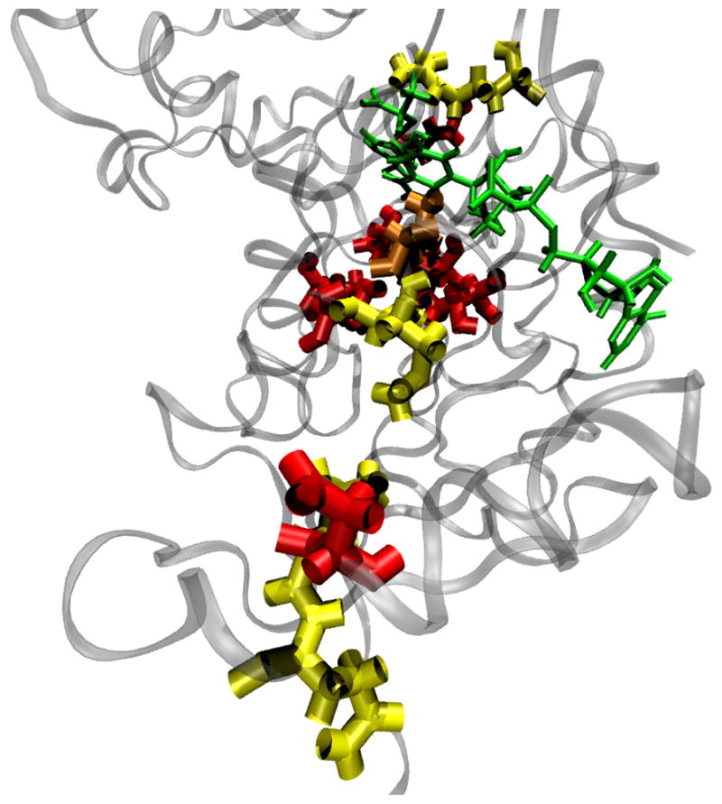
The reaction coordinate found in Ref. 6 is depicted by yellow residues (from front to back: residues 66, 65, 33, 32, 31, 106). The reaction coordinate found by kPCA’s prediction is depicted by red residues (from front to back: residue 64, clustered together are 35, 255, 161, 273, 136, 95 and at the back 192). Residue 31 which is common in both works, is shown as orange. The cofactor and substrate are shown in green color. The importance of the axis along which a compression takes place, has been preserved

To check the prediction of kPCA for the reaction coordinate we selected the residues that were at the minima of Figure 1, constrained them, and as described at the start of this Section, we did a constrained random walk and shot 100 unconstrained trajectories from each of 50 slices, in order to calculate the distribution of the commitment probability. In Figure 2 we show the committor distribution for a transition state found in Ref. 6. Even though the committor distribution is not sharply peaked at 0.5, one should keep in mind that were generated by a statistical algorithm without any other input. The residues that were selected by kPCA could be a good starting point for refining the guess for the reaction coordinate.

Figure 2.

Committor distribution for the residues suggested by the kPCA method for a transition state found in Ref. 6. The kPCA method was able to produce a guess for the reaction coordinate that led to a distribution that has the expected shape.

The most striking feature of the result of Ref. 6 was that the residues we identified as part of the reaction coordinate were along the donor-acceptor axis. The physical explanation is that compressional motions along this axis bring donor and acceptor closer to each other, facilitating the reactive event. It is a crucial test for the kPCA method of identifying the reaction coordinate that it should be able to reproduce this result. In Figure 3 we show the location of the residues identified in the previous work (yellow) and in the current work using kPCA (red), while residue 31, that is commmon in both works, is shown as orange. The cofactor and substrate are shown in green color. We note that the importance of the compressional axis has been preserved. Compared to Ref. 6 there are changes in the specific residues of the axis, but because a protein is a connected polymer, clearly nearby residues may have exactly the same effect in terms of protein dynamics.

4 Conclusion

In conclusion, even after the trajectories that belong to the TPS ensemble have been produced, using only intuition and trial and error for the identification of components of the reaction coordinate still requires several thousands of CPU hours for the calculation of the committor distribution that would verify the correctness of the guess. A method that can produce good guesses for components of the reaction coordinate would be a major help in the analysis of TPS results. In this work we proposed a simple method for identifying components of the reaction coordinate using the kernel PCA method, which has practically no computational requirements and was able to produce a guess that is competitive with the result of our previous TPS analysis.

References

- 1.EW, Ren W, Vanden-Eijnden E. Chem Phys Lett. 2005;413:242–247. [Google Scholar]
- 2.Henkelman G, Johannesson G, Jonsson H. In: Theoretical Methods in Condensed Phase Chemistry. Schwartz SD, editor. Kluwer Academic Publishers; Dordrecht, The Netherlands: 2000. [Google Scholar]
- 3.Bolhuis P, Chandler D, Dellago C, Geissler P. Annu Rev Phys Chem. 2002;53:291–318. doi: 10.1146/annurev.physchem.53.082301.113146. [DOI] [PubMed] [Google Scholar]
- 4.Dellago C, Bolhuis P. Adv Polym Sci. 2009;221:167–233. [Google Scholar]
- 5.Dellago C, Bolhuis P. Top Curr Chem. 2007;268:291–317. [Google Scholar]
- 6.Quaytman S, Schwartz S. Proc Natl Acad Sci USA. 2007;104:12253–12258. doi: 10.1073/pnas.0704304104. [DOI] [PMC free article] [PubMed] [Google Scholar]
- 7.Ma A, Dinner AR. J Phys Chem B. 2005;109:6769–6779. doi: 10.1021/jp045546c. [DOI] [PubMed] [Google Scholar]
- 8.Peters B, Trout BL. J Chem Phys. 2006;125:054108. doi: 10.1063/1.2234477. [DOI] [PubMed] [Google Scholar]
- 9.Peters B, Beckham G, Trout B. J Chem Phys. 2007;127:034109. doi: 10.1063/1.2748396. [DOI] [PubMed] [Google Scholar]
- 10.Rogal J, Lechner W, Juraszek J, Ensing B, Bolhuis P. J Chem Phys. 2010;133:174109. doi: 10.1063/1.3491817. [DOI] [PubMed] [Google Scholar]
- 11.Vreede J, Juraszek J, Bolhuis P. Proc Natl Acad Sci USA. 2010;133:174109. [Google Scholar]
- 12.Best R, Hummer G. Proc Natl Acad Sci USA. 2005;102:6732–6737. doi: 10.1073/pnas.0408098102. [DOI] [PMC free article] [PubMed] [Google Scholar]
- 13.Antoniou D, Schwartz SD. J Chem Phys. 2009;130:151103. doi: 10.1063/1.3123162. [DOI] [PMC free article] [PubMed] [Google Scholar]
- 14.Antoniou D, Basner J, Núñez S, Schwartz SD. Chem Rev. 2006;106:3170–3187. doi: 10.1021/cr0503052. [DOI] [PubMed] [Google Scholar]
- 15.Schölkopf B, Smola A. Learning with kernels: support vector machines, regularization, optimization and beyond. MIT Press; Cambridge, MA: 2002. [Google Scholar]
- 16.Schölkopf B, Smola A, Müller K. In: Advances in kernel methods - support vector learning. Schölkopf B, Burges C, Smola A, editors. MIT Press; Cambridge, MA: 1999. pp. 327–352. [Google Scholar]
- 17.Dellago C, Bolhuis P, Geissler P. In: Computer simulations in condensed matter: from materials to chemical biology (Springer Lecture Notes in Physics) Ferrario M, Ciccotti G, Binder K, editors. Vol. 1. Springer; New York: 2006. pp. 349–391. [Google Scholar]
- 18.Dunn C, Wilks H, Halsall D, Atkinson T, Clarke A, Muirhead H, Holbrook J. Phil Trans R Soc Lond B. 1991;332:117–184. doi: 10.1098/rstb.1991.0047. [DOI] [PubMed] [Google Scholar]
- 19.Fersht A. Structure and mechanism in protein sciences: a guide to enzyme catalysis and protein folding. W. H. Freeman; New York: 1998. [Google Scholar]