A New Three-Dimensional Cephalometric Analysis for Orthognathic Surgery

Abstract

Two basic problems are associated with traditional 2-dimensional ((2D) cephalometry First, many important parameters cannot be measured on plain cephalograms; and second, most 2D cephalometric measurements are distorted in the presence of facial asymmetry. Three-dimensional (3D) cephalometry, which has been facilitated by the introduction of cone beam computed tomography scans, can be solved these problems. However, before this can be realized, fundamental problems must be solved. They are the unreliability of internal reference systems and some 3D measurements, and the lack of tools to assess and measure symmetry. In this manuscript, the authors present a new 3D cephalometric analysis that uses different geometric approaches to solve the fundamental problems previously mentioned. This analysis allows the accurate measurement of the size, shape, position and orientation of the different facial units and incorporates a novel method to measure asymmetry.

Cephalometry is broadly defined as the science of measuring the head of living individuals, although in clinical practice it refers to the analysis of facial form done on a cephalogram. Cephalograms are plain radiographs of the face and cranium taken at a constant distance from the subject with the subject's head stabilized in a cephalostat.^{1, 2} The cephalograms can be obtained in the lateral and frontal views. While many different cephalometric analyses have been developed for the lateral view, a few have been developed for the frontal view.^{3, 4} They have been used to study facial growth and development, to study deformities, to plan orthodontic treatment and surgeries, and to evaluate treatment outcomes.^{3, 5-8}

A given cephalometric analysis is composed of a series of measurements designed to measure the different geometric parameters of the distinct facial units. Four basic parameters can be measured. They are: size, shape, position and orientation. Examples are the Anterior Nasal Spine to Posterior Nasal Spine Distance (ANS-PNS) that measures the size (length) of the maxilla, the Gonial angle (Articulare-Gonion-Menton) that measures the shape of the mandible, Sella-Nasion-Point B (SNB) that measures the anteroposterior position of the mandible and the Maxillary Occlusal Plane Inclination that measures the orientation of the maxilla.

The current standard in cephalometry is to use 2-dimensional (2D) cephalometric analyses based on plain lateral and frontal cephalograms. Unfortunately, the current methods have two basic problems. First, many important parameters cannot be measured on plain cephalograms; and second, most 2D cephalometric measurements are distorted in the presence of facial asymmetry.⁹

The first problem with 2D cephalometry is that the parameters that can be measured on plain cephalograms are limited. An ideal cephalometric analysis should provide 3-dimensional (3D) information regarding the size, shape, position and orientation of the different facial units. However, stand-alone lateral cephalograms can only provide half of the needed information (Table 1). Regarding size, they permit the measurements of length and height, but not of width. Regarding shape, lateral cephalograms can be used to analyze the shape of a unit as seen from the side, but do not permit the evaluation of this parameter from the frontal or submentovertex views. Regarding position, they allow the measurements of the anteroposterior and vertical positions, but not of the transverse. Finally, regarding orientation, they allow the measurement of pitch, but not of roll or yaw.

Table 1.

Lateral Cephalometry

	Length	Height	Width
Size	+++	+++	-
	Sagittal	Coronal	Axial
Shape	+++	-	-
	Anteroposterior	Vertical	Transverse
Position	+++	+++	-
	Pitch	Roll	Yaw
Orientation	+++	-	-

Stand-alone frontal cephalograms also fail to provide half of the needed information (Table 2). In addition, some of the available information from the frontal cephalograms is of poor quality. Regarding size, they only permit the measurements of height and width. Regarding shape, they only allow the evaluation of this parameter from the frontal view. Regarding position, they only allow the measurements of the vertical and the transverse positions. Finally, regarding orientation, they only permit the measurement of roll. Therefore, even if the information from both the lateral and frontal cephalometric analyses is combined, there is still some information that is not available, such as yaw or submentovertex shape (Table 3).

Table 2.

Frontal Cephalometry

	Length	Height	Width
Size	-	+	-
	Sagittal	Coronal	Axial
Shape	-	+	++
	Anteroposterior	Vertical	Transverse
Position	-	+	++
	Pitch	Roll	Yaw
Orientation	-	++	-

Table 3.

Combined Lateral and Frontal Cephalometry

	Length	Height	Width
Size	+++	+++	-
	Sagittal	Coronal	Axial
Shape	+++	+++	++
	Anteroposterior	Vertical	Transverse
Position	+++	+++	++
	Pitch	Roll	Yaw
Orientation	+++	++	-

The second problem with 2D cephalometry is that most 2D cephalometric measurements are distorted in the presence of facial asymmetry. This phenomenon is presented in detail in the accompanying article by the same authors.¹⁰

In order to solve the problems mentioned above, Grayson et al and other researchers^11-14 pioneered the transition from 2D to 3D cephalometry. They combined lateral and frontal 2D cephalograms into a single coordinate system and calculated the 3D coordinates for the cephalometric landmarks. Currently, we are experiencing a paradigm shift as we transition from 2D to 3D imaging. This transition has been facilitated by the introduction of cone-beam computed tomography (CBCT), which allows the acquisition of 3D images in an office setting with a minimal amount of radiation.^15-18 Images obtained by traditional (fan-beam) CT and CBCT scanners can be used to create 3D models of the craniofacial skeleton, the teeth and the soft-tissues.^19-24 By placing these models into the neutral head posture (NHP)^25-29, we can now convert them into “3D cephalograms” in the same way as a lateral head film is consider to be cephalogram if taken at a fixed distance from the subject with the subject's head in a cephalostat.

These new CT-based 3D cephalograms have allowed the further development of 3D cephalometric analyses. ^30-39 However, many important issues with 3D cephalometry remained to be addressed. These problems include the unreliability of internal reference systems and some 3D measurements, and the lack of tools to assess and to measure symmetry. The purpose of this paper is to present a new 3D cephalometric analysis for orthognathic surgery that incorporates solutions to all these problems.

Special Issues in 3D Cephalometry

Unfortunately, 3D cephalometry is much more complex than just adding width to a lateral analysis. As we will discover in the next paragraphs there are several important problems with 3D cephalometry. These include: the reference systems, the way which angles and distances are measured in 3D, and the assessment of symmetry.

Reference Systems

Measuring the head and face requires a frame of reference. In standard 2D cephalometry, a number of different reference planes have been utilized for this purpose. They can be classified as internal or external depending of the location of the elements that define them. Internal reference planes, e.g., Frankfort Horizontal (FH) and Sella-Nasion (S-N), are defined by internal elements like craniofacial bony landmarks, while external planes (e.g., True Horizontal and True Vertical) are defined by external elements such as head posture and the earth's gravitation. Like its 2D counterpart, 3D cephalometry can also use external or internal reference systems.

The internal reference planes (FH, S-N and Basion-Nasion) have several advantages. First, they are not affected by head posture. Second, normative data is available. Third, we are familiar with these reference planes because of the long-time use. In spite of this, internal reference planes have important disadvantages that become apparent when working in 3D space. First, they may be difficult to define. Second, they can be distorted by craniofacial deformity or asymmetry. The first problem is best illustrated by looking at FH. By definition, this plane is demarcated by 4 points. They are the right and left Orbitales and the right and left Porions. However, in a real patient, the likelihood that these four points are located on the same plane (coplanar) is very small. This situation presents a real conundrum since defining a plane using 4 non-coplanar points is physically impossible. Since 3 points define a plane, one option is to leave one of the points out (Fig 1). However, the question then becomes which one? Should it be the right Orbitale, the left Orbitale, the right Porion, or the left Porion? Another option is to average 2 points. However, deciding which 2 points to average is also difficult. A third possible solution is to define the plane as the least squared distance from all the points. The problem with all of these solutions is that some may be ideal for certain patients but not for others. This need for individualization precludes standardization, an important feature of a reference system.

Figure 1.

Frankfurt Horizontal plane on a patient with significant cranial base asymmetry. Both Porions and the right Orbitale are on FH. However, the left Orbitale is above the plane.

The second disadvantage of the internal reference planes is that they can be distorted by craniofacial deformity or asymmetry. This problem can be illustrated by looking at Frankfurt Horizontal on a patient with significant cranial base asymmetry (Fig 1). In such a patient, FH is skewed, and a skewed reference plane will distort all subsequent measurements that depend on it.

Many of these problems can be overcome by using a 3D external reference system (Table 4). The 3 basic reference planes used in anatomy are well suited for this purpose. They are the midsagittal, the coronal and the axial planes. The midsagittal plane passes through the facial midline and divides the face into right and left halves. The coronal plane passes through both external auditory canals and divides the face into anterior and posterior halves. And the axial plane passes through both external auditory canals and divides the face into upper and lower portions. These planes are perpendicular to each other (orthogonal) and are defined by the head posture, the earth's gravitation and the visual axis (Fig 2). In 3D graphics, a reference system such as this is referred to as the “world coordinate system”. These planes are easy to define and are not altered by facial deformity or asymmetry. However, they are reliable only if the head is oriented in the Neutral Head Posture. The NHP is the position of the head where the head in neither flexed nor extended, neither rotated nor tilted. A most convenient way of capturing the NHP is by using a digital orientation device^{26, 40-42} as described by the authors in an accompanying article in this journal.²⁸

Table 4.

General rules of an ideal 3D cephalometric analysis for orthognathic surgery

Reference Systems	1. Build a world coordinate system for the whole head 2. Build a local coordinate system for each unit
Orientation	1.Compare the orientation of the local with the world coordinate systems 2. Measure yaw, remove yaw; measure roll, remove roll; and, measure pitch
Size	Length, Height or Width Measure distances in 3D space. The distance measurements can be done between any combination of points, lines or planes
Position	Anteroposterior and Vertical Project all landmarks on the world midsagittal plane before the measurements (both angle and distance)
	Transverse Measure the distance between the landmark and the world midsagittal plane
Shape	3D	Measure directly in 3D space.
	2D	Unit's profile shape
			Side	1. Project landmarks on the local midsagittal plane 2. Report bilateral measurements separately
			Front	1. Project landmarks on the local coronal plane 2. Report bilateral measurements separately
			Bottom	1. Project landmarks on the local axial plane 2. Report bilateral measurements separately

Figure 2.

A 3D external reference system. The 3 orthogonal reference planes are used: the midsagittal, the coronal and the axial.

3D Measurements

The majority of cephalometric measurements are angles between 2 lines, angles between lines and planes, angles between 2 planes, distances between a point and a line, or distances between 2 points. Conventionally, we have measured these items in 2 dimensions. However, a 3D cephalometric analysis requires that we measure them in 3 dimensions. Measuring these angles and distances in 3D is significantly different that measuring them in 2D. Moreover, a 3D measurement may have a different meaning that it's 2D counterpart. In the following sections, we describe how these different items are measured in 3 dimensions and the shortcomings of some of these measurements.

Line-Line Angles

The interincisal angle is an angle between 2 lines: the long axis of the maxillary central incisor (U1) and the long axis of the mandibular central incisor (L1). This measurement can be used as an example of how line to line angles are measured in 3 dimensions. The 3D angle between two lines is measured by the equation $\theta =\text{acos}\frac{a\cdot b}{\mid a\mid \ast \mid b\mid }$, where a and b are the vectors pointing in the direction of each line. Although this equation may be of interest to some, for most clinicians, the important issue is how these 3D measurements can impact their clinical decisions. These clinical implications are best understood by looking at the results of a simple experiment illustrated in Fig 3. Figs 3A and 3B present an ideal interincisal angle: the long axes of the upper and lower incisors are oriented to each other, so the pitch between them is 130°, the yaw is 0° and the roll is 0°. As expected, the measured 3D interincisal angle is 130°. In Figs 3C and 3D, we rotated the lower incisor around an anteroposterior axis to produce 15° of roll while the pitch remained at 130° and the yaw remained at 0°. This transformation changed the 3D interincisal angle to 128°, which was 2° smaller than previously measured. The results of this experiment indicate the differences between the conventional 2D measurements and the new 3D measurements. In 2D, we always interpret the interincisal angle as the pitch between the upper and lower incisors. An angle of 128° means that the pitch between the incisors is lower than the mean (i.e., 130°). However, in 3D this angle is actually a composite of pitch, roll and yaw. Therefore, a 3D interincisal angle of 128° may be produced by many different combinations of these parameters and it can no longer be interpreted as the pitch between the upper and lower incisors.

Figure 3.

An example illustrates how a 3D line-line angle is measured.

A) The blue line is the U1 and the orange line is the L1. The pitch of L1 to U1 is 130°, and the roll and the yaw are 0° respectively.

B) The lateral view of (A).

C) The L1 is rolled clockwise by 15°, while the pitch remains at 130° and the yaw remains at 0°. The 3D interincisal angle is now changed to 128°.

D) The lateral view of (C).

Line-Plane Angles

The inclination of the maxillary central incisor to Frankfurt Horizontal is an angle between a line (long axis of the upper incisor) and a plane (FH). This measurement can be used as an example of how line-to-plane angles are measured in 3 dimensions. The 3D line-plane angles are calculated by first determining the plane's normal vector (Fig 4) and then using the equation for 2 lines to compute the angle between the normal vector and the line. A normal vector is a vector that is perpendicular to the plane. It can be calculated by the cross product (a × b) of 2 vectors lying on the plane. Given 2 coplanar vectors and a and , x = (Ya * Zb) – (Yb * Za), y = (Za * Xb) – (Zb * Xa), and z = (Xa * Yb) – (Xb * Ya). The clinical implications of these measurements are best understood by looking at the results of a simple experiment illustrated in Fig 5. Figs 5A and 5B present an ideal U1-FH angle. The long axis of the maxillary central incisor is oriented to FH at a pitch of 113°, a roll of 0° and a yaw of 0°. As expected, the measured 3D angle between U1 and FH is 113°. In Figs 5C and 5D we rotated the maxillary incisor around an anteroposterior axis to produce a 10° roll while the pitch remained at 113° and the yaw remained at 0°. This transformation changed the 3D U1-FH angle to 115°, which was 2° larger than previously measured. The results of this experiment indicate the differences between the conventional 2D measurements and the new 3D measurements. In 2D, we always interpret the U1-FH as the pitch of the upper incisors in relation to Frankfort Horizontal. An angle of 115° means that the upper incisors are too proclined. However, in 3D this angle is actually a composite of pitch, roll and yaw. Therefore, a 3D U1-FH angle of 115° may be produced by many different combinations of these parameters and it can no longer be interpreted as the pitch of the upper incisor.

Figure 4.

A normal vector (black arrow) is a vector that is perpendicular to the surface of the plane.

Figure 5.

An example illustrates how a 3D line-plane angle is measured.

A) The blue line is the U1. The plane depicted in yellow is FH. The yellow line is the normal vector of the FH plane. The pitch of the U1 to FH is 113°, and the roll and the yaw are 0° respectively.

B) The lateral view of (A). The 3D U1-FH angle is 113°.

C) The maxilla is rolled clockwise by 10°, while the pitch remains at 113° and the yaw remains at 0°. The 3D axial inclination of the maxillary central incisor is now changed to 115°.

D) The lateral view of (C).

Plane-Plane Angles

The inclination of the maxillary occlusal plane to FH is an angle between 2 planes. This measurement can be used as an example of how plane to plane angles are measured in 3 dimensions. The 3D plane-plane angles are calculated by first determining the planes’ normal vectors and then using the equation for 2 lines to compute the angle between them. The clinical implications of these measurements are best understood by looking at the results of the experiment illustrated in Fig 6. Figs 6A and 6B present an ideal maxillary occlusal plane angle: the maxillary occlusal plane is oriented to FH at a pitch of 7°, roll of 0° and yaw of 0°. As expected, the measured 3D angle is 7°. In Figs 6C and 6D, we rotated the maxillary occlusal plane around an anteroposterior axis to produce a 10° roll while the pitch remained at 7° and the yaw remained at 0°. However, this transformation changed the 3D maxillary occlusal plane angle to 12°, which was 5° larger than previously measured. The results of this experiment indicate the differences between the conventional 2D measurements and the new 3D measurements. In 2D, we always interpret the maxillary occlusal plane angle as the pitch of the maxillary occlusal plane in relation to FH. An angle of 12° means that the maxillary orientation is too steep. However, in 3D this angle is actually a composite of pitch, roll and yaw. Therefore, a 3D maxillary occlusal plane angle of 12° may be produced by many different combinations of these parameters and it can no longer be interpreted as the pitch of the maxillary occlusal plane.

Figure 6.

An example illustrates how a 3D plane-plane angle is measured.

A) The blue line is the normal vector of the maxillary occlusal plane. The orange line is the normal vector of the FH plane. The pitch of maxillary occlusal plane to FH is 7°, and the roll and the yaw are 0° respectively.

B) The lateral view of (A).

C) The maxilla is rolled clockwise by 10°, while the pitch remained at 7° and the yaw remained at 0°. The 3D maxillary occlusal plane to FH angle is now changed to 12°.

D) The lateral view of (C).

Point-Line Distances

Ricketts Convexity of Point A is measured as the distance between a point (Point A) and a line (Nasion-Pogonion). This measurement can be used as an example of how point-line distances are calculated in 3 dimensions. The 3D distance between a point and a line is computed using the equation $d=\frac{\mid (p-a)\times v}{\mid v\mid }$, where p is the position vector for the point, a is the position vector for the line, and v is the direction vector for the line. The clinical implications of these measurements are best understood by looking at the results of the experiment illustrated in Fig 7. Figs 7A and 7B presents an ideal convexity where Point A is 2 mm in front of the Nasion-Pogonion line. In this ideal condition, Points A, Nasion and Pogonion are located on the midsagittal plane. In Figs 7C and 7D, we moved Point A 4 mm to the right to produce an asymmetry, while the anteroposterior and vertical position of this point did not change. We then remeasured the Ricketts Convexity and found it to be 4.5 mm, which was 2.5 mm greater than perviously measured. In 2D cephalometry, Ricketts Convexity is a measurement of relative anteroposterior position. However, the same is not true in 3D. The results of this experiment indicate that the 3D convexity measurement may change even if the anteroposterior relationship between the landmarks does not change. In clinical practice, we are required to assess the position of the facial units on each individual axis of space: anteroposterior, vertical and transverse. However, angles and distances measured in 3D space may not provide such information.

Figure 7.

An example illustrates how a 3D point-line distance is measured.

A) An ideal Ricketts Convexity is measured when Points A, Nasion and Pogonion are located on the sagittal plane. Point A is 2 mm in front of the N-Pg line.

B) The lateral view of (A).

C) The submental vertex view of (A).

D) Point A is moved 4 mm to the right to produce an asymmetry, while the anteroposterior and vertical position of this point remained the same. Ricketts Convexity is now changed to 4.5 mm, resulting in 2.5 mm greater than before.

E) The lateral view of (D)

F) The submental vertex view of (D)

The Problem of 3D Measurements in Facial Asymmetry

In the previous examples, we saw that 3D cephalometric measurements can be distorted by adding roll or moving a unit transversely in 3D space. Although not illustrated above, the same can also occur with yaw. Since abnormal roll, yaw or transverse position of a facial unit produces facial asymmetry, it can be inferred that in patients with facial asymmetry, direct 3D measurements can be unreliable. Measurements of orientation, position and shape can be affected by this problem. In the following subsections we will discuss a solution to these problems.

Solution to the Orientation Problem

The decision making process in orthognathic surgical planning requires that we separately asses the pitch, roll and yaw of each facial unit. However, as discussed above, composite 3D angles cannot be used for this purpose. After months of investigation, we discover that we can separately measure the pitch, roll and yaw by constructing an individual coordinate system for each facial unit or element. We call these systems local coordinate systems to differentiate them from the world coordinate system, which is used to orient the whole head (Table 4). In this approach, each individual facial unit, i.e., maxilla, mandible and chin, has its own local coordinate system. The local coordinate systems are defined around each unit's intrinsic plane of symmetry and can be automatically constructed by computer software. Fig 8 illustrates how this is done for the maxilla. In the first step (Fig 8A), a maxillary occlusal plane is built for the maxillary dental arch. Three points define this plane. They are the right and left mesiobuccal cusps of the upper first molars (UR6 and UL6) and the incisal embrasure between the upper central incisors (UIE). In the second step (Fig 8B), the computer calculates a normal vector of this plane. As discussed above, a normal vector is a vector that is perpendicular to the plane. This vector represents the vertical (z) axis of the local coordinate system. In the third step (Fig 8C), the computer calculates the local anteroposterior (y-) axis. This axis passes through UIE and bisects a line that goes from UR6 to UL6. The y-axis is the local axis of symmetry of the maxilla. In the last step (Figs 8D and 8E), the computer calculates the transverse (x-) axis of the local coordinate system. This axis is perpendicular to z- and y- axes.

Figure 8.

An example illustrates how a local coordinate system is built.

A) In the first step, a maxillary occlusal plane is defined by 3 points, UR6, UL6 and UIE.

B) In the second step, the computer calculates a normal vector of this plane. The vector represents the vertical (z-) axis of the local coordinate system.

C) In the third step, the computer calculates the local anteroposterior (y-) axis. This axis passes through UIE and bisects a line that goes from UR6 to UL6. It is the local axis of symmetry of the maxilla.

D) In the last step, the computer finally calculates the transverse (X-) axis of the local coordinate system. This axis is perpendicular to Z and Y axes.

E) The 3D view of maxillary local coordinate system.

After the computer software builds all the local coordinate systems, it measures the pitch, roll and yaw of each unit by comparing the orientation of each local axis with the corresponding axis of the world coordinate system. However, this is not as simple as it may seem. To calculate these angles it is necessary to measure them in a specific order. Fig 9 illustrates how the pitch, roll and yaw for the maxilla are measured. First, the algorithm measures the yaw. This angle is the angle between the x axis of the local coordinate system and the X axis of the world coordinate system as they are projected on the axial plane (Y-X plane, Fig 9A). After the yaw is calculated, the algorithm removes the yaw by rotating the local coordinate system around the center of origin aligning the local x and world X axes (Fig 9B). Following this, the computer measures the roll, which is the angle between the local z and the world Z axes as they are projected on the coronal plane (Z-X plane, Fig 9C). The algorithm then removes the roll by rotating the local axes around the origin to align the local z and world Z axes (Fig 9D). Finally, the computer measures the pitch, which is the difference between the local y and world Y axes (Fig 9E).

Figure 9.

The pitch, roll and yaw of a facial unit (e.g., maxilla) can be measured by comparing the orientation of the local coordinate system (color arrows) with the world coordinate system (black lines). The origin of the local coordinate system is UIE. The yellow arrow is the transverse (x) axis, the red is the anteroposterior (y) axis, and the blue arrow is the vertical (z) axis.

A) The first step is to measure the yaw, which is the angle between x axis of the local coordinate system and the X axis of the world coordinate system as they project on the axial plane (Y-X plane, submental vertex view).

B) After the yaw is calculated, the algorithm rotates the local coordinate system around the center of origin aligning the local x the world X axes (removing the yaw, submental vertex view).

C) It illustrates the frontal view of the maxilla at the same orientation as in B). After the yaw is removed, the second step is to measure the roll, which is the angle between the local z axis and the world Z axis as they project on the coronal plane (Z-X plane).

D) The computer program then rotates the local axes around the origin to align the local and world Z axes (removing the roll, frontal view). E) The last step is to measure the pitch, which is the angle between the local y axis and the world Y axis (right view).

Solution for the Position Problem

The position of a facial unit can be measured using distances or angles (Table 4). Examples of distances include Ricketts Convexity and the Wits Appraisal, while examples of angles include Facial Angle and SNB. In patients with facial asymmetry, the involved cephalometric landmarks can be displaced away from the midsagittal plane in the transverse direction. The displacement can change the value of a 3D measurement, even if the actual anteroposterior position of the landmarks is unchanged. This creates a problem for the clinicians, who may have difficulties interpreting the meaning of these 3D measurements. For the angle measurements, these distortions are relatively small and may be clinically insignificant.⁹ However, as shown above, for distances these distortions are larger and may be significant.

In our new cephalometric analysis, we solve this problem by first projecting the involved landmarks on the midsagittal plane and then measuring the angles or distances in 2 dimensions.^{9, 30} This approach is simple and works well for position measurements. Another advantage of this approach is that it conserves many of the time-proven 2D measurements.

Solution for the Shape Problem

The shape of an object is independent from its size, position and orientation. Therefore, the measurement of the shape should not be influenced by these variables. However, in traditional 2D lateral cephalometric analyses, some of the shape measurements will be distorted if the involved facial units are asymmetrically oriented.¹⁰ As an example, the Gonial Angle can be distorted if the mandible has a roll or a yaw deformity. The Gonial Angle is a 2D angle formed by the projection of the points Condylion, Gonion and Menton on the midsagittal plane, and is utilize to describe the shape of the mandible as seen laterally. When the mandible is tilted, the projected angle changes even though the shape of the actual mandible does not (Fig 10).

Figure 10.

In this example, we measure the Gonial Angle (shape) of a mandible with intrinsic symmetry. The local coordinate system of the mandible is shown as a bounding box. The local midsagittal plane is in middle of the bounding box. Although the mandible should be projected to both local and world midsagittal planes, for the purpose of demonstration, the 2D projection on the local midsagittal plane is moved to the right side of the bounding box, while the 2D projection on the world midsagittal plane is moved to the left side of the world coordinate system.

A) When both yaw and roll of the mandible are 0°, the local coordinate system of the mandible is completely parallel to the world coordinate system. Therefore, the 2D projection of the mandible on the local midsagittal plane (red) is the same as the one on the world midsagittal plane (blue). Both projected Gonion Angles are measured at 127°.

B) When we rotate the mandible to produce 20° of yaw while the roll remains at 0°, the local coordinate system is no longer parallel to the world coordinate system. The Gonial Angle projected on the local midsagittal plane remains the same at 127° (red) because its local coordinate system is rotated together with the mandible. However, the Gonial Angle projected on the world midsagittal plane is distorted and increased to 130° (blue).

This problem can be solved by directly measuring these angles in 3D. However, 3D shape analyses are complex and we currently lack the necessary normative data to interpret them. At present, a practical solution to this problem is to measure the shape as a projected 2D image in a way that prevents distortions. This can be done by projecting the involved landmarks onto the local midsagittal planes rather than the midsagittal plane of the world coordinate system (Fig 10). The local midsagittal plane is defined by the local y and z axes. The advantage of using the local coordinate systems over the world coordinate system is that they rotate together with their objects preventing projection distortions.

Symmetry

Symmetry refers to a pattern of self-similarity. Although there are many different types of symmetries, the one we are concerned with is reflection-symmetry, also known as mirror-image symmetry or bilateral symmetry. This type of symmetry occurs when 2 halves of a whole are each other's mirror images. For a 3D object, symmetry occurs around a plane.⁴³

One may consider that symmetry is an all-or-none phenomenon. This notion has little value in our field since most faces have some degree of asymmetry. For the majority of individuals, the face has a rough bilateral symmetry with respect to the midsagittal plane. Although no individual face is perfectly symmetrical, the degree of asymmetry is usually minor. However, major deviations in symmetry are considered pathological and are commonly observed in different types of dentofacial deformities.^{44, 45}

Two conditions must be met for facial symmetry to occur. First, the individual facial units (e.g., maxilla, mandible, and chin) must have intrinsic symmetry. Second, the units must be positioned symmetrically with respect to the sagittal plane. If these conditions are not met, the result is asymmetry. A simple and useful method to quantify symmetry is to measure the minimal transformation that is needed to achieve symmetry (Fig 11).⁴⁶ Our new 3D cephalometric analysis utilizes this principle to measure the degree of intrinsic symmetry of the different facial units, and to measure the degree of symmetric alignment of these units with respect to the midsagittal plane.

Figure 11.

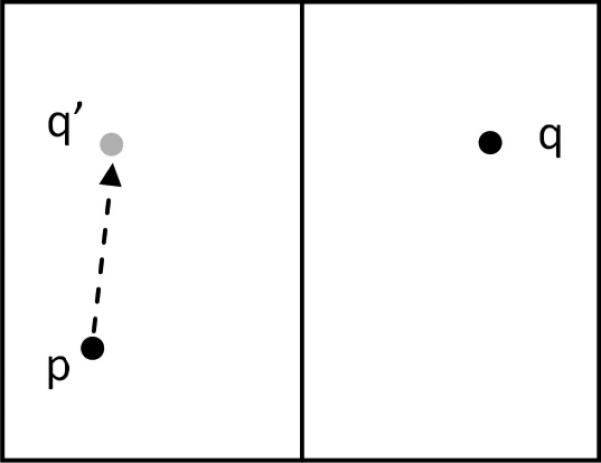
A simple method to quantify symmetry by measuring the minimal transformation needed to achieve symmetry.

A) Two points, p and q are located asymmetrically on each side of a vertical axis.

B) The degree of asymmetry between p and q can be quantified by first creating a mirror-imaged point q’, which is symmetrical with q.

C) The minimum distance between p and q’ is a measurement of the degree of asymmetry between the points.

The degree of intrinsic symmetry of the maxillary and mandibular dental arches can be measured by constructing triangles with vertices located on the right and left mesiobuccal cusps of the first molars and on the incisal embrasures between the 2 central incisors.^{9, 11, 12, 45, 47} In patients with symmetric dental arches, this triangle is an isosceles triangle with 2 equal sides and 2 equal angles. The equal sides are located between the incisal embrasure and the first molars, and the 2 equal angles are located at the first molars. In patients with asymmetric arches, this triangle is a scalene triangle with 3 different sides and 3 different angles. A simple way of quantifying the degree of intrinsic asymmetry is to calculate the difference between the 2 base angles, which are located at the first molars (Fig 12). The larger the difference is, the larger the degree of asymmetry. The main advantage of this approach is that this measurement is not influenced by jaw size. Another advantage is its simplicity. The degree of intrinsic symmetry of the basal mandible can also be measure using this method. This can done by constructing a triangle with vertices located at right and left Gonion, and Menton.

Figure 12.

Method to measure the intrinsic symmetry of the maxilla.

A) Maxillary dental arch triangle as seen from the submental-vertex view.

B) The middle triangle is generated by a dental arch with perfect symmetry. Symmetric dental arches generate isosceles triangles. These triangles have 2 equal sides and 2 equal angles. A dental arch is considered to have intrinsic symmetry if the base angles are identical (β-γ = 0).

C) The triangle on the far right is generated an asymmetric dental arch. Asymmetric dental arches generate scalene triangles. In a scalene triangle all sides and all angles are different. The degree of intrinsic asymmetry of a dental arch can be quantified by measuring the difference between the base angles (β-γ ≠ 0).

As stated above, facial asymmetry can also be the result of the misalignment of a facial unit with respect to the midsagittal plane. When a unit is not symmetrically aligned, the degree of misalignment (i.e., asymmetry) can be quantified by measuring the transformations (i.e., translations and rotations) needed to realign this unit. Three parameters relate to symmetric alignment. They are: transverse position, roll and yaw. Fig 13 illustrates this concept. In this example, the maxilla is asymmetrically positioned with respect to the midsagittal plane. The magnitude of this misalignment can be quantified by measuring the transverse dental midline deviation (e.g., 4 mm), the roll (e.g. 8°) and the yaw (e.g., 5°).

Figure 13.

The degree of symmetric misalignment can be quantified by measuring the transformations (translations and rotations) necessary to achieve symmetric alignment using 3 factors: transverse position, roll and yaw.

A) As seen from the frontal view, the midline deviation of the maxillary dental arch is 4mm and the roll is 8° in this example.

B) As seen from the submental-vertex view, the yaw of the maxillary dental arch is 5°.

The New 3D Cephalometric Analysis

Rational

The goal of our new 3D cephalometric analysis is to maintain all the positive aspects of conventional 2D analysis while addressing its negative aspects. This has been accomplished by incorporating different strategies to solve the problems of direct 3D measurements (Table 4). All cephalometric measurements are classified into 4 different groups (size, shape, position and orientation) according to the parameter they measure. In our new analysis, size is measured as a linear distance in 3D space. Shape is measured by projecting the involved landmarks onto the midsagittal plane of the local coordinate system for each facial unit. Position is measured differently depending upon the direction of the measurements. The transverse position is measured as a linear distance between the involved landmark and the midsagittal plane of the world coordinate system. The anteroposterior and vertical positions are measured after all the involved landmarks have been projected onto the midsagittal plane of the world coordinate system. Finally, orientation is measured as separate pitch, roll and yaw for each facial unit. This is done by comparing the orientations of the local and world coordinate systems.

The analysis is divided into 6 components: symmetry, transverse, vertical, pitch, anteroposterior and shape (Table 5). The order of these sections mimics the ideal order in which a 3D surgical plan should be developed. The symmetry analysis is novel, while the other five components incorporate time-proven measurements. The new analysis also incorporates data gathered during the physical examination. The concept behind this analysis is to have all the necessary information needed to plan a surgery in a single report. Finally, this analysis is meant to be modular. The important aspects of the analysis are its concepts and structure. The measurements presented here are the ones that we have found useful. We encourage others to adapt this analysis to their needs by adding, deleting or replacing measurements (rows) or by adding new elements or units (columns).

Table 5.

Our new 3D cephalometric analysis for orthognathic surgery (a shadowed space indicates the input from the clinical examination).

#: All the norms were established for Caucasian subjects with normal facial appearance. All the norms for symmetry analyses were based on the authors’ opinion. The hard tissue norms were established by Bhatia and Leighton for 20 year-old subjects⁴⁹, with the exceptions of following: Ricketts norms were established by Ricketts for 9 year-old subjects⁴, ⁵⁰, ⁵¹; Maxillary Occlusal Plane Inclination was established by Downs⁵², ⁵³; and Holdaway Ratio was based on Holdaway's opinion⁵⁴-⁵⁷. The soft tissue norms were established by Farkas for 20 to 26 year-old subjects⁵⁸, with the exceptions of following: Incisal Show was based on the authors’ opinion; lip measurements were established by Peck et al for 15.5 year-old subjects who were either in orthodontic treatment or posttreatment⁵⁹, ⁶⁰; and Posterior Airway Space was established by Riley et al for male subjects⁴⁸. The dental arch norms were established by Moyers et al for 18 year-old subjects⁶¹.

§: This is the original Ricketts norm established for 9-year-old subjects. No age adjustment is required.

†: The norm is calculated for FH plane. Please use with caution.

‡: This is the original Downs norm established for “Occlusal Plane to FH” (“Cant of Occlusal Plane” in Downs's original manuscript⁵²). The occlusal plane was defined as a line bisecting the occluded mesiobuccal cusps of the upper and lowers first molars and the incisal overbite. Please use with caution.

¶: The gonial angle is measured by projecting the landmarks Articulare, Gonion and Menton to the mandibular local midsagittal plane.

*: Posterior Airway Space should be measured as the shortest distance between the tongue base and the posterior pharyngeal wall. The norm was established by Riley for measuring the distance between the 2 landmarks: Tongue Base (TB, the intersection point of a line from Point B through Gonion and the base of the tongue), and Posterior Pharyngeal Wall (PPWB, the intersection point of a line from Point B through Gonion and the base of the posterior pharyngeal wall). Please use with caution.

Abbreviations:

M: Male;

F: Female;

MSP: Midsagittal plane;

UIE: Upper central incisal embrasure;

LIE: Lower central incisal embrasure;

Pg: Pogonion (the most anterior point on the mandibular symphysis);

UR6: Mesiobuccal cusp of maxillary right first molars;

UL6: Mesiobuccal cusp of maxillary left first molar;

LR6: Mesiobuccal cusp of mandibular right first molars;

LL6: Mesiobuccal cusp of mandibular left first molar;

Ral and Lal: Right and Left Alar (the most lateral points on the right and left alar contour)

Ren and Len: Right and Left Endocanthion (a point at the inner canthus of the eyelids);

Tr: Trichion (the point on the hairline in the midsagittal plane of the forehead);

G’: Soft Tissue Glabella (the most prominent or anterior point in the midsagittal plane of the forehead at the level of the superior orbital ridges);

Sn: Subnasale (a point located at the junction between the columnella of the nose and the skin of the upper lip at the midsagittal plane);

Me’: Soft Tissue Menton (the most inferior point on the midline of the soft tissue chin);

ULS: Upper lip stomion (the most inferior point of the midline of the upper lip vermillion);

LLS: Lower lip stomion (the most superior point of the midline of the lower lip vermillion);

ANS: Anterior Nasal Spine (the tip of the anterior nasal spine);

Xi: Ricketts Xi landmark (the midpoint of the right and left inferior alveolar nerve foramens);

PM: Suprapogonion (a point at which the shape of the symphysis metalis changes from convex to concave – also known as protuberance menti);

U1: Long axis of maxillary central incisors (a line connects the upper central incisal embrasure and the midpoint of right and left upper central incisal apices);

AxP: Axial plane (the true Horizontal plane);

Go: Gonion (the midpoint at the mandibular angle);

ME: Menton (the lowest point on the lower border of the mandibular symphysis);

MP: Mandibular Plane (a plane constructed by the landmarks Me, right Go and left Go);

L1: Long axis of mandibular central incisors (a line connects the lower central incisal embrasure and the midpoint of right and left lower central incisal apices);

S: Sella (the center of sella turcica);

N: Nasion (the most anterior point on the frontonasal suture);

A: Point A: The deepest point on the concave outline of the upper labial alveolar process extending from the anterior nasal spine to prosthion;

B: Point B: The deepest point on the bony curvature between the crest of the alveolus (infradentale) and pogonion;

Cm: Columella (the most anterior point on the columella of the nose);

Ls: Laberale Superius (a point located at the maximum convexity of the vermilion border most prominent in the midsagittal plane);

Co: Condylion (the most posterosuperior point of the mandibular condyle).

Symmetry

This part of the analysis measures the symmetry of the maxilla, the mandible and the chin. The symmetry analysis is divided into 2 parts. The first part measures the intrinsic symmetry and the second part measures the degree of symmetric alignment of the facial units with respect to the midsagittal plane. To measure the intrinsic symmetry of the maxilla, we utilize the technique previously described in Fig 12. The degree of intrinsic symmetry of the maxillary dental arch is measured as the difference between the 2 base angles located at the first molars. A value of zero indicates perfect intrinsic symmetry. The larger the deviation is from “0”, the higher the degree of asymmetry.

The intrinsic symmetry of the mandible is measured by assessing the symmetry of 2 separate triangles: a mandibular dental arch triangle and a mandibular basal bone triangle. The mandibular dental arch triangle is analogous to the maxillary dental arch triangle and bound by the vertices located at the tip of the right and left mesiobuccal cusp of the mandibular first molar (LR6 and LL6), and the mandibular dental midline (LIE). The vertices of the mandibular basal bone triangle are located at right and left Gonion, and Menton. As mentioned above, the degree of mandibular intrinsic symmetry is measured as the difference between the 2 base angles located at the first molars and Gonion, respectively.

The second part of the symmetry analysis measures the degree of symmetric alignment of the different facial units. The degree of symmetric alignment of the maxilla is quantified by first measuring, in millimeters, the transverse (right-left) deviation of the upper incisal embrasure to the midsagittal plane. Any deviation from this plane produces asymmetry and is consider abnormal. A deviation to the right is recorded as a positive number and a deviation to the left as a negative number. The next 2 steps in the symmetry analysis are to measure the degree of yaw and roll of the maxilla. Yaw is defined as a rotation around the vertical (z-) axis which produces buccal corridor asymmetry. The degree of yaw is measured by calculating the amount of rotation necessary to place UR6 and UL6 equidistant from the midsagittal plan. As seen from the submental-vertex view, a positive angle denotes a clockwise rotation of the maxilla and a negative angle a counterclockwise rotation. A value of “0” denotes yaw symmetry and is considered normal. Roll is defined as a rotation around the anteroposterior (y-) axis which produces a cant. The degree of roll is measured by calculating the amount rotation around UIE that is required to place UR6 and UL6 on the same vertical position. As seen from the front, a positive angle denotes a clockwise rotation of the maxilla and a negative angle a counterclockwise rotation. A value of “0” denotes roll symmetry and is consider normal.

Measuring symmetric alignment of the mandible is similar to the maxilla. However, in addition to measuring the symmetric alignment of the dental arch, we also measure the symmetric alignment of its basal bone (right and left Gonion, and Menton).

To measure the symmetric alignment of the chin, we first measure the horizontal distance between Pogonion and the midsagittal plane. Afterwards, we calculate the degree of roll and yaw of this unit using a local coordinate system. To build this system, a basal chin triangle is first constructed. The vertices of this triangle are Menton, and the right and left Posterior Chin (PC-R and PC-L) points. These points have been created specifically for this analysis, and are located on the inferior border of the mandible, 2 cm from Menton (Fig 14). The vertical axis of the local coordinate system is a vector that originates at Menton and is perpendicular to the surface of the triangle. In addition, the anteroposterior axis originates at Menton and bisects the distance between PC-R and PC-L Points. Finally, the transverse axis, which also originates at Menton, is perpendicular to the vertical and anteroposterior axes.

Figure 14.

Chin local coordinate system.

PC-R (right posterior chin point), PC-L (left posterior chin point) and Menton define the basal chin triangle. The yellow arrow is the local transverse (x-) axis, the red arrow is the anteroposterior (y-) axis and the blue arrow the vertical (z-) axis.

To interpret the measurements of chin symmetry, it is important to compare them to the measurements for the mandible. A separate chin surgery to correct an asymmetry is only indicated if the chin asymmetry is not corrected after repositioning the mandible. Comparable degrees of asymmetry (roll and yaw) between the mandibular occlusal triangle and the chin triangle indicate that the chin asymmetry will be corrected by mandibular surgery.

Transverse

While certain transverse measurements (e.g. midline deviations) reflect symmetry, others (e.g. width measurements) do not. All symmetry related transverse measurements have been incorporated in to the symmetry analysis. This section is reserved for non-symmetry related transverse measurements. In our analysis, we measure the intercanthal distance, the alar base width, and the maxillary and mandibular intermolar widths. We have selected these measurements because we have found them useful during planning. At the time of a LeFort I osteotomy, a surgeon can control the width of the alar base with alar cinch suture. The need and extent of this maneuver are influenced by the presurgical alar width, it's relation to the intercanthal distance, and the patient's race. The intermolar width has been selected because it is a measurement of the transverse size of the jaws.

Vertical Measurements

In this section of the analysis, vertical measurements are presented separately for the maxilla, mandible and chin. For the maxilla, the analysis determines the adequacy of its vertical position. Of all the measurements that can be used for this purpose, the most clinically relevant are the ones that relate the vertical position of the maxillary incisors to the upper lip. To determine the norm of this relationship, clinicians should take following into account: age and gender of the patient, length of the upper lip, amount of incisal show at rest, amount of gingival show during smiling, presence or absence of delayed passive eruption, and amount of incisal attrition.

For the mandible, the analysis establishes the normality of its vertical position. For simplicity we have included a few measurements. The analysis measures the amount of overbite and calculates Ricketts Lower Facial Height (ANS-Xi-PM).

Pitch Measurements

The next part of the analysis determines the pitch of the different maxillofacial units. Since deviations in pitch have profound effects on the anteroposterior projection of the jaws, the assessment of pitch should always precede the anteroposterior assessment. In our analysis, the pitch of the maxilla is quantified by measuring the inclination of the maxillary occlusal plane and the inclination of the maxillary central incisors as they relate to the Axial Plane.

The mandibular pitch is quantified by measuring the inclinations of the mandibular plane as they relate to the Axial Plane, as well as the inclination of the mandibular central incisors to the mandibular plane, and the interincisal angle.

Anteroposterior Measurements

The anteroposterior measurements are completed separately for the maxilla, mandible and chin. In addition, we also quantify the anteroposterior discrepancies between the maxilla and the mandible. Measurements such as the Wits appraisal, ANB and Ricketts Convexity of Point A are utilized for this purpose. To quantify the anteroposterior position of the maxilla, we measure Maxillary Depth, SNA and the Nasolabial Angle. For the mandible, we determine the Facial Angle, SNB and the Posterior Airway Space⁴⁸. Finally, for the chin we calculate the Holdaway Ratio.

Shape

The last part of the analysis evaluates the shape of the different facial units. Currently, the only shape measurement that we routinely use is the Gonial Angle. In the future, we plan to develop tools to assess shape in three dimensions. We encourage others to do the same.

References

- 1.Broadbent BH. A new X-ray technique and its application to orthodontia: The introduction of cephalometric radiography. Angle Orthod. 1931;1:45. [Google Scholar]
- 2.Broadbent BH, Broadbent BH, Jr., Golden WH. Bolton standards of dentofacial development growth. V.V. Mosby; Saint Louis: 1975. [Google Scholar]
- 3.Proffit WR, Fields HW, Jr., Ackerman JL, et al. Contemporary orthodontics. 3rd ed. Mosby; St. Louis: 2000. [Google Scholar]
- 4.Athanasiou AE. Orthodontic cephalometry. Mosby-Wolfe; St. Louis: 1995. [Google Scholar]
- 5.Bell WH, Guerrero CA. Distraction Osteogenesis of the Facial Skeleton. 1st ed. BC Decker, Inc; 2006. [Google Scholar]
- 6.Gliddon MJ, Xia JJ, Gateno J, et al. The accuracy of cephalometric tracing superimposition. J Oral Maxillofac Surg. 2006;64:194. doi: 10.1016/j.joms.2005.10.028. [DOI] [PubMed] [Google Scholar]
- 7.Enlow DH, Hans MG. Essentials of facial growth. W.B. Saunders; Philadelphia: 1996. [Google Scholar]
- 8.Ricketts RM. Philosophies and methods of facial growth prediction. Proc Found Orthod Res. 1971:11. [PubMed] [Google Scholar]
- 9.Xia JJ, Gateno J, Teichgraeber JF. New clinical protocol to evaluate craniomaxillofacial deformity and plan surgical correction. J Oral Maxillofac Surg. 2009;67:2093. doi: 10.1016/j.joms.2009.04.057. [DOI] [PMC free article] [PubMed] [Google Scholar]
- 10.Gateno J, Xia JJ, Teichgraeber JF. Effect of facial asymmetry on common cephalometric measurements: A 2-dimensional and 3-dimensional study. J Oral Maxillofac Surg. 2010;68 doi: 10.1016/j.joms.2010.10.046. in- press. [DOI] [PMC free article] [PubMed] [Google Scholar]
- 11.Grayson B, Cutting C, Bookstein FL, et al. The three-dimensional cephalogram: theory, technique, and clinical application. Am J Orthod Dentofacial Orthop. 1988;94:327. doi: 10.1016/0889-5406(88)90058-3. [DOI] [PubMed] [Google Scholar]
- 12.Grayson BH, McCarthy JG, Bookstein F. Analysis of craniofacial asymmetry by multiplane cephalometry. Am J Orthod. 1983;84:217. doi: 10.1016/0002-9416(83)90129-x. [DOI] [PubMed] [Google Scholar]
- 13.Cutting C, Bookstein FL, Grayson B, et al. Three-dimensional computer-assisted design of craniofacial surgical procedures: optimization and interaction with cephalometric and CT-based models. Plast Reconstr Surg. 1986;77:877. doi: 10.1097/00006534-198606000-00001. [DOI] [PubMed] [Google Scholar]
- 14.Zhu M, Cai Z, Zhang LY, et al. Establishment of 3D analysis system of craniomaxillofacial skeketon. Chinese J Oral Maxillofac Surg. 1998;8:15. [Google Scholar]
- 15.Kau CH, Richmond S, Palomo JM, et al. Three-dimensional cone beam computerized tomography in orthodontics. J Orthod. 2005;32:282. doi: 10.1179/146531205225021285. [DOI] [PubMed] [Google Scholar]
- 16.Scarfe WC, Farman AG, Sukovic P. Clinical applications of cone-beam computed tomography in dental practice. J Can Dent Assoc. 2006;72:75. [PubMed] [Google Scholar]
- 17.White SC, Pharoah MJ. Oral Radiology: Principles and Interpretation. 4th ed. Mosby; St. Louis, MI: 2000. [Google Scholar]
- 18.Scarfe WC, Farman AG, Levin MD, et al. Essentials of maxillofacial cone beam computed tomography. Alpha Omegan. 2010;103:62. doi: 10.1016/j.aodf.2010.04.001. [DOI] [PubMed] [Google Scholar]
- 19.Gateno J, Xia J, Teichgraeber JF, et al. A new technique for the creation of a computerized composite skull model. J Oral Maxillofac Surg. 2003;61:222. doi: 10.1053/joms.2003.50033. [DOI] [PubMed] [Google Scholar]
- 20.Xia J, Ip HH, Samman N, et al. Three-dimensional virtual-reality surgical planning and soft-tissue prediction for orthognathic surgery. IEEE Trans Inf Technol Biomed. 2001;5:97. doi: 10.1109/4233.924800. [DOI] [PubMed] [Google Scholar]
- 21.Xia J, Samman N, Yeung RW, et al. Computer-assisted three-dimensional surgical planing and simulation. 3D soft tissue planning and prediction. Int J Oral Maxillofac Surg. 2000;29:250. [PubMed] [Google Scholar]
- 22.Swennen GR, Mollemans W, Schutyser F. Three-dimensional treatment planning of orthognathic surgery in the era of virtual imaging. J Oral Maxillofac Surg. 2009;67:2080. doi: 10.1016/j.joms.2009.06.007. [DOI] [PubMed] [Google Scholar]
- 23.Swennen GR, Mommaerts MY, Abeloos J, et al. A cone-beam CT based technique to augment the 3D virtual skull model with a detailed dental surface. Int J Oral Maxillofac Surg. 2009;38:48. doi: 10.1016/j.ijom.2008.11.006. [DOI] [PubMed] [Google Scholar]
- 24.Farman AG, Scarfe WC. Development of imaging selection criteria and procedures should precede cephalometric assessment with cone-beam computed tomography. Am J Orthod Dentofacial Orthop. 2006;130:257. doi: 10.1016/j.ajodo.2005.10.021. [DOI] [PubMed] [Google Scholar]
- 25.Schatz EC. A new technique for recording natural head position in three dimensions (MS thesis) In: Xia JJ, English JD, Garrett FA, et al., editors. Orthodontics. The University of Texas Health Science Center at Houston; Houston: 2006. [Google Scholar]
- 26.Schatz EC, Xia JJ, Gateno J, et al. The development of a new technique of recording and transferring natural head position (NHP) in three dimensions. J Craniofac Surg. 2010;21 doi: 10.1097/SCS.0b013e3181ebcd0a. In press. [DOI] [PubMed] [Google Scholar]
- 27.Weiskircher MN. Accuracy of a new technique for recording natural head position in three dimensions. In: Xia JJ, English JD, Bouquot JE, et al., editors. Orthodontics. The University of Texas Health Science Center at Houston; Houston: 2007. [Google Scholar]
- 28.Xia JJ, McGrory JK, Gateno J, et al. Clinical feasibility of recording natural head position in three-dimension. J Oral Maxillofac Surg. 2010;68 in-press. [Google Scholar]
- 29.McGrory JK. In: Clinical feasibility of a new technique for recording naturan head position in three dimensions (MS Thesis) Xia JJ, English JD, McGrory KR, et al., editors. The University of Texas Health Science Center at Houston; Houston: 2008. [Google Scholar]
- 30.Swennen GR, Schutyser F, Hausamen J-E. Three-Dimensional Cephalometry: A Color Atlas and Manual. Springer-Verlag; Berlin: 2005. [Google Scholar]
- 31.Moerenhout BA, Gelaude F, Swennen GR, et al. Accuracy and repeatability of cone-beam computed tomography (CBCT) measurements used in the determination of facial indices in the laboratory setup. J Craniomaxillofac Surg. 2009;37:18. doi: 10.1016/j.jcms.2008.07.006. [DOI] [PubMed] [Google Scholar]
- 32.Swennen GR, Schutyser F. Three-dimensional cephalometry: spiral multi-slice vs cone-beam computed tomography. Am J Orthod Dentofacial Orthop. 2006;130:410. doi: 10.1016/j.ajodo.2005.11.035. [DOI] [PubMed] [Google Scholar]
- 33.Swennen GR, Schutyser F, Barth EL, et al. A new method of 3-D cephalometry Part I: the anatomic Cartesian 3-D reference system. J Craniofac Surg. 2006;17:314. doi: 10.1097/00001665-200603000-00019. [DOI] [PubMed] [Google Scholar]
- 34.van Vlijmen OJ, Berge SJ, Swennen GR, et al. Comparison of cephalometric radiographs obtained from cone-beam computed tomography scans and conventional radiographs. J Oral Maxillofac Surg. 2009;67:92. doi: 10.1016/j.joms.2008.04.025. [DOI] [PubMed] [Google Scholar]
- 35.Olszewski R, Reychler H, Cosnard G, et al. Accuracy of three-dimensional (3D) craniofacial cephalometric landmarks on a low-dose 3D computed tomograph. Dentomaxillofac Radiol. 2008;37:261. doi: 10.1259/dmfr/33343444. [DOI] [PubMed] [Google Scholar]
- 36.Olszewski R, Villamil MB, Trevisan DG, et al. Towards an integrated system for planning and assisting maxillofacial orthognathic surgery. Comput Methods Programs Biomed. 2008;91:13. doi: 10.1016/j.cmpb.2008.02.007. [DOI] [PubMed] [Google Scholar]
- 37.Olszewski R, Zech F, Cosnard G, et al. Three-dimensional computed tomography cephalometric craniofacial analysis: experimental validation in vitro. Int J Oral Maxillofac Surg. 2007;36:828. doi: 10.1016/j.ijom.2007.05.022. [DOI] [PubMed] [Google Scholar]
- 38.Park SH, Yu HS, Kim KD, et al. A proposal for a new analysis of craniofacial morphology by 3-dimensional computed tomography. Am J Orthod Dentofacial Orthop. 2006;129:600, e23. doi: 10.1016/j.ajodo.2005.11.032. [DOI] [PubMed] [Google Scholar]
- 39.Hwang HS, Hwang CH, Lee KH, et al. Maxillofacial 3-dimensional image analysis for the diagnosis of facial asymmetry. Am J Orthod Dentofacial Orthop. 2006;130:779. doi: 10.1016/j.ajodo.2005.02.021. [DOI] [PubMed] [Google Scholar]
- 40.Xia JJ, Gateno J, Schatz EC, et al. Accuracy of a new technique for recording natural head position in three dimensions. 90th Annual Meeting of American Association of Oral and Maxillofacial Surgeons.; Seattle, WA. September 17-20, 2008. [Google Scholar]
- 41.Schatz EC. Department of Orthodontics. The University of Texas Health Science Center at Houston; Houston, TX: 2006. A new technique for recording natural head position in three dimensions (M.S. Thesis) [Google Scholar]
- 42.Weiskircher MN. Department of Orthodontics. The University of Texas Health Science Center at Houston; Houston, TX: 2007. Accuracy of a new technique for recording natural head position in three dimensions (M.S. Thesis) [Google Scholar]
- 43.Pan G, Wang Y, Qi Y, et al. Proceedings of the 18th International Conference on Pattern Recognition. IEEE Computer Society; Hong Kong, China: 2006. Finding symmetry plane of 3D face shape. [Google Scholar]
- 44.Epker BN, Stella JP, Fish LC. Dentofacial deformities. Mosby; St. Louis: 1995. [Google Scholar]
- 45.Gateno J, Xia JJ, Teichgraeber JF, et al. Clinical feasibility of computer-aided surgical simulation (CASS) in the treatment of complex cranio-maxillofacial deformities. J Oral Maxillofac Surg. 2007;65:728. doi: 10.1016/j.joms.2006.04.001. [DOI] [PubMed] [Google Scholar]
- 46.Ras F, Habets LL, van Ginkel FC, et al. Method for quantifying facial asymmetry in three dimensions using stereophotogrammetry. Angle Orthod. 1995;65:233. doi: 10.1043/0003-3219(1995)065<0233:MFQFAI>2.0.CO;2. [DOI] [PubMed] [Google Scholar]
- 47.Xia JJ, Gateno J, Teichgraeber JF. Three-dimensional computer-aided surgical simulation for maxillofacial surgery. Atlas Oral Maxillofac Surg Clin North Am. 2005;13:25. doi: 10.1016/j.cxom.2004.10.004. [DOI] [PubMed] [Google Scholar]
- 48.Riley R, Guilleminault C, Herran J, et al. Cephalometric analyses and flow-volume loops in obstructive sleep apnea patients. Sleep. 1983;6:303. doi: 10.1093/sleep/6.4.303. [DOI] [PubMed] [Google Scholar]
- 49.Bhatia SN, Leighton BC. A manual of facial growth: A computer analysis of longitudinal. cephalometric growth data. 1st ed. Oxford University Press; New York: 1993. [Google Scholar]
- 50.Ricketts RM. Perspectives in the clinical application of cephalometrics. The first fifty years. Angle Orthod. 1981;51:115. doi: 10.1043/0003-3219(1981)051<0115:PITCAO>2.0.CO;2. [DOI] [PubMed] [Google Scholar]
- 51.Ricketts RM, Roth RH, Chaconas SJ, et al. Orthodontic diagnosis and planning: their roles in preventive and rehabilitative dentistry. Rocky Mountain Orthodontics; 1982. [Google Scholar]
- 52.Downs WB. Variations in facial relationships: their significance in treatment and prognosis. Am J Orthod. 1948;34:812. doi: 10.1016/0002-9416(48)90015-3. [DOI] [PubMed] [Google Scholar]
- 53.Downs WB. The role of cephalometrics in orthodontic case analysis and diagnosis. Am J Orthod. 1952;38:162. [Google Scholar]
- 54.Holdaway RA. The relationship of the bony chin and the lower incisor to the line NB (in a postgraduate course, University of California) 1955 [Google Scholar]
- 55.Holdaway RA. Angle Society conference. Pasadena, CA: 1957. A consideration of the soft tissue outline for diagnosis and treatment planning. [Google Scholar]
- 56.Freeman RB. Are Class II elastics necessary? Am J Orthod. 1963;49:165. [Google Scholar]
- 57.Steiner CC. The use of cephalometrics as an aid to planning and assessing orthodontic treatment. Am J Orthod. 1960;46:721. [Google Scholar]
- 58.Farkas LG, editor. Anthropometry of the head and face. 2nd ed. Ravan Press; New York: 1994. [Google Scholar]
- 59.Peck S, Peck L, Kataja M. Some vertical lineaments of lip position. Am J Orthod Dentofacial Orthop. 1992;101:519. doi: 10.1016/0889-5406(92)70126-U. [DOI] [PubMed] [Google Scholar]
- 60.Peck S, Peck L, Kataja M. The gingival smile line. Angle Orthod. 1992;62:91. doi: 10.1043/0003-3219(1992)062<0091:TGSL>2.0.CO;2. [DOI] [PubMed] [Google Scholar]
- 61.Moyers RE, van der Linden FPGM, Riolo ML, et al. Standards of human occlusal development. Center for Human Growth and Development, The University of Michigan; Ann Arbor: 1976. [Google Scholar]