SIMCON—simulation control to optimize man-machine interaction

SUMMARY

The fitting of mathematical models to physiological systems can be tedious and difficult, whether one uses analog or digital computer methods. Both methods have their pros and cons depending on the available hardware and software and on the type of modeling. In recent years many digital simulation languages have been written combining analog-like and digital features to facilitate modeling, but, for a variety of reasons, none of these was suitable for our applications. We, therefore, designed a new digital simulation control system, SIMCON, which is described in this paper.

The primary objectives were to provide:

1. Maximum man-machine interaction at run-time, including visual displays, digital control, and both continuous analog and digital parameter adjustment

2. The ability to generate solutions and to fit them to experimental data or other theoretical curves with a minimum of computer memory

3. The option to use a mathematically oriented language, FORTRAN, and block operators with variable input/output.

The result is a relatively general and simple simulation system which is easy to use and has wide versatility.

INTRODUCTION

The fitting of mathematical models to physiological systems can be tedious or difficult when using either analog or digital methods. Typically, analog simulations require relatively long setup time and some care in time and amplitude scaling, but they provide high solution speed, visual output, and easy changing of parameters. While digital solutions are easy to program, and while hard copy output and greater accuracy may be obtained digitally, the serial nature of digital computation makes solutions slow, and there are seldom adequate means for making immediate visual assessments of the solutions or for making adjustments to the model or its parameters. Many digital simulation languages that combine features of both analog and digital machines have been written in recent years in attempts to facilitate the solution of such problems as model fitting. However, after studying several of these languages, we concluded that none was suitable for our applications, for a variety of reasons—most lacked on-line operational flexibility, many were not compatible with our particular hardware and software configurations, some had extravagant memory requirements, involved long or special setup procedures, lacked a variety of input/output characteristics, etc.

The objectives of the digital simulation system (SIMCON) were (1) maximum man-machine interaction at run time including visual displays, digital control, and both continuous analog and digital parameter adjustment, (2) the ability to generate solutions and to fit them to experimental data or other theoretical curves without using large amounts of computer memory, and (3) the combined use of a mathematically oriented language, FORTRAN, and block operators with variable inputs and outputs.

DESCRIPTION

General

SIMCON was designed for use with a CDC 3200 computer, a time-sharing monitor (a modified MEDLAB¹), one tape drive, one disk pack, a printer, a card reader, analog-to-digital and digital-to-analog converters, and a Calcomp plotter. Program execution is initiated from a peripheral computer station consisting of a decimal keyboard and a memory oscilloscope (Figure 1). SIMCON, written in basic assembly language, BAP, provides a means of investigator-model interaction via digital and analog input/output, while taking full advantage of the time-sharing monitor.

Figure 1.

A computer terminal consisting of an oscilloscope, a keyboard and a potentiometer-controlled parameter entry device

The mathematical model is programmed in FORTRAN II and after compilation is stored on the magnetic disk with an identifying number. When the FORTRAN program number is entered with the decimal keyboard, SIMCON loads the program into memory and controls its execution. Control parameters and data that must be addressed by both SIMCON and the FORTRAN program are stored in the common area of memory.

The control of SIMCON (see flow chart, Figure 2) is almost entirely accomplished by use of parameter options, i.e., the investigator manipulates the flow of the program by setting certain controlling parameters to the “on” or “off” position. Some of these on/off options are illustrated as decision blocks (black diamonds) accompanied by the controlling parameter number. One hundred “parameters” (P₁₀₀ to P₂₀₀) are associated with control functions within SIMCON and the first hundred are available for use in the user’s FORTRAN program (see Figure 3). Any of the parameters can be displayed on the memory oscilloscope or written on magnetic tape or the Calcomp plotter.

Figure 2.

Block diagram of SIMCON. The numbers beside the decision blocks (black diamonds) indicate which parameter is set to control the program route. For example, P₁₀₉ would be set positive if the user wishes to read the analog line voltages controlled by the analog potentiometers.

Figure 3.

SIMCON parameter functions

The control parameters and the user’s parameters can be adjusted either prior to or during a solution, by any of several means:

1. Card input prior to a solution

2. Decimal keyboard in conjunction with a memory oscilloscope at one of the remote stations

3. Analog potentiometers

4. Automatic parameter adjustment loops

5. The FORTRAN program itself.

Figures 4a and 4b are typical messages on the memory oscilloscope showing the means of computer-to-user communication afforded by SIMCON. The combination of digits shown on the left of Figure 4a is entered on the keyboard at the remote terminal to direct the flow of the program. An entry on the keyboard preceded by a 1 is recognized as a parameter index; an entry preceded by a 2 is recognized as a new parameter value. If the user enters an incorrect value from the keyboard, he may depress the SOM (start of message) key, which allows the entry of a new value. Figure 4b shows the oscilloscope message received when parameter 57 was set to a new value from the remote terminal.

Figure 4.

(a) One of the messages transmitted by SIMCON prior to an operator decision. SOM and EOM are keyboard codes for start and end of message, respectively, (b) Reply from SIMCON after a new value has been entered for parameter 57.

Modeling program

The program for mathematical modeling is written in FORTRAN with all the standard features (I/O, function subroutines, etc.) available, but control is exerted by the user at a peripheral station. Subroutines may be written in the usual way, and a growing number of block operator subroutines (integrators of several types, linear and parabolic interpolation, fixed and continuously variable delays, function generators, etc.) are available as FORTRAN subroutines. While we have chosen to use FORTRAN as the working language, there is no reason that we could not have used another, more specialized simulation language.

The FORTRAN program is similar to those used with the SCi continuous system simulation language² in that it has three parts: (1) an initial region, (2) a dynamic or solution-generating region, and (3) a terminal region.

The initial region is executed once at the beginning of a solution and sets the initial conditions for the solution. If variable, these initial conditions can be entered with the decimal keyboard.

The terminal region of the FORTRAN program is used to make a quantitative assessment of the solution and to produce a permanent record of the solution on chosen output devices.

Any variable that is selected at run time can also be displayed graphically on the memory oscilloscope during the solution, with new points being added with each step increase of the independent variable (usually time). Parameters used in the FORTRAN program can be altered via the keyboard prior to and during generation of the solution to determine solution sensitivities to parameter changes. Experimental or other data arrays that have been previously stored on the magnetic disk may be displayed on the memory oscilloscope for visual comparison with the solutions obtained from a model. The stored arrays may also be variable functions used in obtaining the solution, usually after interpolation. When repetitive solutions are being obtained, up to 10 computed values for each solution may be written on digital tape for later display or analysis. (The number 10 was arbitrarily chosen to meet our present requirements and could readily be increased.)

Control loops

External to and nested around the innermost solution loop are three other loops (see Figure 2), each of which may be functional or nonfunctional as determined by parameter options. The first is an “analog potentiometer loop” by means of which parameters take values either prior to or during a solution from 4 potentiometers whose outputs are converted to digital values for use during a solution. The analog signals (0 to 3 volts DC) are generated by batteries within the box shown above the oscilloscope in Figure 1 and are transmitted to the digital computer via a 10-bit analog-to-digital converter. Each potentiometer has three controlling parameters associated with it. The first specifies which one of the two hundred parameters is to be changed during a solution, and the other two are chosen maximum and minimum values for the parameter which is to be altered. The value of the specified parameter is the chosen minimum plus the fraction of the potentiometer range times the difference between the maximum and the minimum. The potentiometers allow a more rapid adjustment of parameter values between iterations than could be obtained by digital entry of new values, and they can be continuously varied during a solution.

The other two outer loops are used to make predetermined arithmetic or logarithmic adjustments of 2 selected parameters. Parameters may also be adjusted under program control—for example, after assessment of the solution in the third portion of the user’s program.

Output

Hard copy graphical output for display of variables is obtainable by means of (a) the memory scope, which can be photographed, (b) Calcomp graphs, or (c) printer plots. The same methods are available for plotting results from many solutions stored on digital tape—for example, for plotting the amplitude of output of an operator against the frequency of a repetitive input function. The arrays stored on tape may also be displayed rapidly on the memory scope using arithmetic or logarithmic scaling, thus allowing a quick check of results or choice of appropriate scaling for permanent graphing.

Applications

Many processes in biological research can be approached by describing the transfer function of the system whose input and output can be measured experimentally. This is the classical problem of system identification; it may be attacked in various ways, depending in part on whether the system is a simple open-loop network or a multiple-feedback closed-loop system. An illustration is the problem of obtaining a description of the transport function, the probability density function of transit times of material carried in the bloodstream between an upstream point A and a downstream point B. Let some indicator which travels with the blood be injected upstream and its concentration in the blood at A and B be recorded as A(t) and B(t), respectively. Using SIMCON, the transport function from A to B can be obtained accurately and with relative ease based on the assumption that this transport function can be approximated with what may be described as a variable-order low-pass filter whose impulse response is overdamped. This last requirement is important since negative concentrations cannot exist.

Figure 5 is a block diagram of the FORTRAN program for the variable-order model used to simulate the transport function. A(t) and B(t) represent the digitized upstream and downstream indicator dilution curves that have been read into memory from the magnetic disk. Many pairs of curves may reside on the disk, and a particular pair is selected with SIMCON parameter options. Operators FIRST and SECORD approximate dispersion plus transport delay, while DELAY is an operator that approximates delay alone. All operator parameters, initial conditions, damping coefficients (ZETA), natural frequencies (OMEGA), time constants (TAU), and delays (DLAY) are set according to SIMCON parameter values. Parameters 89 and 90 are the outputs of scaling summers, and parameter 71 is the “integral” of the square of the differences between two functions used to measure curve ”fit.” The linkages between these operators are quite variable, and as long as the step size in the independent variable (time) is small, then the order of listing in the program is of little consequence. A linkage such as given by the dashed lines must be used, certain operators remaining unused. When the parameters of the model have been adjusted so that its output response to an input having the form of the upstream dye curve closely approximates the recorded downstream dye curve, then the impulse response of the model can be generated by substituting a short duration pulse, parameter 82, as the input to the model.

Figure 5.

Diagram of operators available in program 7540. Dashed lines show possible configuration chosen at run time.

The FORTRAN model program is shown below to illustrate its simplicity. The initializing, solution generating, and solution assessing sections of the program are shown, as is the scheme for linking the operators.

Figure 6 shows an upstream indicator dilution curve, C_A(t), and an output of the model, labeled C_A(t) * h(t), which was compared with an experimentally recorded downstream indicator dilution curve C_B(t). The parameters of the model were varied, using the keyboard at a remote computer terminal, until the differences between the theoretical and the experimental output curves were minimized; when the differences were less than a predetermined tolerance, the model was said to approximate the transport function, h(t). A third-order filter plus a time delay was used to obtain this fit, one SECORD (ZETA = 0.85, OMEGA = 1.20), one FIRST (TAU = 0.70), and one DELAY (DLAY = 5.20) all in series.

Figure 6.

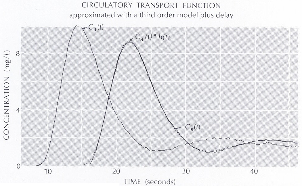
Upstream, C_A(t), and downstream, C_B(t), dilution curves are shown along with a theoretical downstream curve (dashed line) obtained using a simulated transport function, h(t)

The goodness of fit between C_B(t) and C_A(t) * h(t) was determined visually on the memory oscilloscope and improved by minimizing the sums of squares of the differences between the computed solution and the experimental curve. This particular transport function description required approximately five minutes for parameter adjustment. Since the updated parameter list is stored with the FORTRAN program on the magnetic disk, successive fits of similar functions require less iteration time for the selection of an optimum model and model parameters. This program thus contained more operators than were necessary, but this excess provided wide latitude in choosing and testing a variety of models. Having chosen a suitable model as a result of such testing, one should then rewrite the program omitting the unnecessary operators.

In feedback systems such as might be formulated at least crudely using a general program (such as program 7540 or Figure 5), the phase lags introduced by inappropriate sequencing of the operators can be partly overcome by using a very small step size in obtaining the solutions. After choosing a better defined model the sequencing of the operators should be changed to minimize undesired phase lags and to permit the use of larger step sizes.

In another application, SIMCON was used to define magnitudes of potential errors in estimating flow, mean transit time, dispersion, and volume by the standard dye dilution techniques introduced by fluctuations in flow.³ The adjustable parameters included the frequency, phase and amplitude of the sinusoidal flow, shaping parameters of the dispersive delay operator, the average flow, the form of the simulated tracer input, and many others including the selection of output variables and output devices. Other applications have been in testing models for capillary-tissue exchange and analyzing data obtained from dogs for permeability of capillary membranes in the heart⁴ and for the extent of counter-current diffusional exchange of water in the heart.⁵

CONCLUSION

In general, SIMCON is very useful in finding the solution to any problem where repeated man-machine interaction is essential because logical adjustments are difficult or impossible to define in advance. Most obvious are the iterative methods of solution where error functions are difficult to program or define before the solution is initiated. SIMCON provides the programming ease, accuracy, memory, and hard copy output of digital computing and yet allows the man-machine interaction and run-time flexibility usually associated with analog computing.

Biographies

DENNIS U. ANDERSON was born in Waseca, Minnesota in 1942. In 1964 he received his BS degree from St. Olaf College at Northfield, Minnesota, where he majored in biology with minors in math and chemistry. Shortly thereafter he joined the Department of Physiology at the Mayo Clinic, where he was introduced to simulation and computer work. In ’68 and ’69 he was a systems programmer for UNIVAC in Roseville, Minnesota and was assigned to the 1108 FORTRAN V compiler. Just recently he has rejoined the Mayo Clinic, where his primary concern is simulation and real-time I/O programming.

THOMAS J. KNOPP writes: “I was born in 1938 in Winona, Minnesota, where I completed my grade and high school education. I was first introduced to formal simulation in the U.S. Air Force, where I served as an instructor and electronics technician for electronic instrument flight simulators, an aircraft emergency procedures simulator, and an air-to-ground missile guidance simulator. With my appetite for electronics and mathematics whetted, I obtained a BA degree from Winona State College, with majors in mathematics and physics. I have since been a member of a cardiovascular research group in the Physiology Department, Mayo Clinic, Rochester, Minnesota, while pursuing an MS degree from the Biophysics Department, University of Minnesota. My research is concerned primarily with the description of material transport, using simulation techniques to elucidate transport phenomena.”

J. B. BASSINGTHWAIGHTE was born in Toronto in 1929. He took his MD at the University of Toronto in 1955 and, after being in the general practice of medicine in northern Ontario, undertook postgraduate training in Internal Medicine at the Postgraduate Medical School of London, England, and at the Mayo Clinic. This led him into physiology and to a PhD (1964), combining training at Mayo and at the University of Minnesota (Mayo is a part of the Graduate School). Beginning with electrical analogs of circulatory transfer functions in work with Homer R. Warner, modeling (analog, digital, and hybrid) soon became, for Dr. Bassingthwaighte, a practical tool in the quantitative analysis of physiological phenomena.

He is a member of Simulation Councils, Inc., as well as the American Physiological Society, the Biophysical Society, and the Biomedical Engineering Society.

REFERENCES

- 1.Pryor TA, Warner HR. Time sharing. In: Moshman J, editor. Datamation. Washington D C: Thompson Book Company; 1966. Apr, p. 54. [Google Scholar]
- 2.SCi Simulation Software Committee. The SCi continuous system simulation language (CSSL) SIMULATION. 1967. Dec, [Google Scholar]
- 3.Bassingthwaighte JB, Anderson DU, Knopp TJ. Effects of unsteady flow on indicator dilution in the circulation; Proceedings 19th Annual Conference on Engineering in Medicine and Biology; 1966. p. 184. [Google Scholar]
- 4.Bassingthwaighte JB, Knopp TJ, Hazelrig JB. In: Crone C, Lassen NA, editors. A concurrent flow model for capillary-tissue exchange Alfred Benzon II Symposium on Capillary Permeability; Copenhagen: 1969. in press. [Google Scholar]
- 5.Yipintsoi T, Knopp TJ, Bassingthwaighte JB. Concurrent exchange of labelled water in canine myocardium; Federation Proceedings vol 28 no 2 p 645; Federation of American Societies of Experimental Biology; 1969. Mar, [Google Scholar]