Predicted Interval Plots (PIPS): A Graphical Tool for Data Monitoring of Clinical Trials

Abstract

Group sequential designs are often used in clinical trials to evaluate efficacy and/or futility. Many methods have been developed for different types of endpoints and scenarios. However, few of these methods convey information regarding effect sizes (e.g., treatment differences) and none uses prediction to convey information regarding potential effect size estimates and associated precision, with trial continuation. To address these limitations, Evans et al. (2007) proposed to use prediction and predicted intervals as a flexible and practical tool for quantitative monitoring of clinical trials. In this article, we reaffirm the importance and usefulness of this innovative approach and introduce a graphical summary, predicted interval plots (PIPS), to display the information obtained in the prediction process in a straightforward yet comprehensive manner. We outline the construction of PIPS and apply this method in two examples. The results and the interpretations of the PIPS are discussed.

1. Introduction

Many group sequential methods have been proposed to monitor clinical trials with different types of endpoints and scenarios. However, few of these methods convey information regarding effect sizes (e.g., treatment differences) and none uses prediction to convey information regarding potential effect size estimates and associated precision, with trial continuation. To overcome these limitations, Evans et al. (2007) proposed to use prediction and predicted intervals as a flexible and practical tool for quantitative monitoring of clinical trials. In this article, we reaffirm the importance and usefulness of this innovative approach and introduce a graphical summary, predicted interval plots (PIPS), to display the information obtained in the prediction process in a straightforward yet comprehensive manner. In Section 2, we briefly review existing group sequential methods. In Section 3, we introduce a method to construct predicted intervals for time-to-event endpoints and discuss the construction of PIPS. In Section 4, we apply our approach in two examples. We will end with a discussion in Section 5.

2. Background and Motivation

In clinical trials, the data are prospectively accumulated over a period of time. Group sequential designs are a natural choice to ensure that the trial is properly executed and there are no severe safety concerns associated with the therapies. Group sequential methods also allow timely evaluation of superiority or futility so that the trial could be stopped early when appropriate to save valuable resources.

Several group sequential methods have been developed. Pocock (1977) and O’Brien and Fleming (OF, 1979) proposed the first two formal group sequential methods to evaluate the mean difference between two treatment groups when the responses are normally distributed with known variance. Both methods were designed to test between the null hypothesis (H₀) that the mean treatment difference is zero and the alternative hypothesis (H_A) that it is nonzero. Under the null hypothesis, using Pocock’s test, it is equally likely to reject H₀ at all interim analyses, while in OF’s test, it is much easier to reject H₀ at the later interim analyses than the earlier ones. Subsequently, researchers have extended their work to offer stopping boundaries with alternative shapes (Wang and Tsiatis 1987); to adapt to other response distributions (Harrington et al. 1982; Tsiatis 1982) through justifying normal approximations to the joint distributions of the test statistics; and to allow unequal and unpredictable increments of group sizes or other generalizations to fit realistic settings (Slud and Wei 1982; Lan and DeMets 1983; Kim and DeMets 1987). In some of the group sequential designs, the trial is only allowed to stop early to reject the null hypothesis (i.e., stop early for efficacy only). Thus, the stopping boundaries are constructed such that the overall probability of ever rejecting the null hypothesis during the trial when H₀ is true, the Type I error rate α, is well preserved under a nominal level (e.g., 0.05). However, for economic concerns of saving time and resources and ethical concerns of preventing study participants from being exposed to ineffective therapies, it is also important to allow the trial to stop early for futility (Berntsen 1991; Chang 2004). As a consequence, multiple tests have been proposed (Gould and Pecore 1982; Pampallona and Tsiatis 1994; Pampallona et al. 2001) to permit early stopping under the null hypothesis by specifying a set of lower stopping boundaries. That is, if the test statistic crosses the lower stopping boundary, the trial will be terminated and the null hypothesis will be accepted. Lower stopping boundaries are constructed such that the Type II error rate β of wrongly accepting the null hypothesis is well preserved below a nominal level. Whitehead and his collaborators also proposed the triangular test and the double triangular test for one-sided and two-sided group sequential tests respectively (Whitehead and Stratton 1983; Whitehead 1997).

Each of these group sequential methods is based on hypothesis testing. Therefore, they are subject to limitations including: (1) the significance levels (i.e., p-values) do not convey information regarding precision and effect size; and (2) they have inflexible decision rules that do not allow incorporation of other data (e.g., other endpoints, safety data) into the decision process. More flexible approaches have been proposed such as repeated confidence intervals (RCIs) and stochastic curtailment. The former approach, proposed by Jennison and Turnbull (1984, 1985), addresses the first limitation by constructing a sequence of confidence intervals (one at each interim look) with a sequence of simultaneous (joint) coverage probabilities specified based on an α-spending function (Jennison and Turnbull 2000). The width and the location of the confidence intervals explicitly convey the precision of the estimate as well as the estimated effect size. The stochastic curtailment approach addresses the second limitation by defining the criterion for early stopping for futility based on a measure of the probability of rejecting the null hypothesis at the final analysis (Lan et al. 1982; Choi et al. 1985). The conditional power in the frequentist paradigm and the predictive power in the Bayesian paradigm are two such measures, which can be combined with other data such as the safety data to aid decision making. However, neither approach addresses both limitations. Moreover, all the aforementioned methods derive inference for the parameter of interest using the observed interim data. None of them evaluates the potential gain in precision and power with trial continuation to give the investigators a better understanding of the pros and cons associated with the decision to continue or terminate the trial.

Motivated by these limitations, Evans et al. (2007) proposed a new flexible monitoring tool for clinical trials using predicted intervals, a prediction of the confidence intervals for our parameter of interest at some future time point t_f (e.g., the end of study). The innovation of this approach is the idea of simulating the yet-to-be-observed data between now and t_f based on reasonable assumptions. Then, the predicted intervals will be constructed from the observed data and the simulated future data using standard methods. This approach has many appealing features. The gain of precision with trial continuation and the associated increase in sample size will be reflected in the length of the predicted intervals. Sensitivity analyses can be conducted by varying the data-generating assumptions. The possibility of yielding a significant test, if the trial continues to t_f, can be adequately evaluated under different assumptions. This information can then be used with other data such as safety data to help make decisions.

In this article, we introduce a new graphical summary based on the predicted intervals: the predicted interval plots (PIPS). The construction of PIPS is described in detail in Section 3.2. Briefly, to account for the random variation in the data-generating process, under each assumption regarding the future unobserved data, the simulation process is repeated many times each time resulting in a predicted interval. Then all of the predicted intervals are plotted based on the predicted point estimates. By doing so, the probability of rejecting the null hypothesis at the specified future time point t_f if the trial continues (i.e., the conditional power) can be obtained directly from the plot for any data-generating assumption. Moreover, the variation in the predicted point estimates and the variation in the length of the predicted intervals are explicitly displayed in the plot. PIPS can be created and compared for any future time points and for different data-generating assumptions to aid in the decision-making process.

3. Predicted Intervals and Predicted Interval Plots

The heuristic ideas behind the predicted interval approach are straightforward and apply naturally to binary, continuous, and time-to-event endpoints. They can be applied in superiority and noninferiority trials. Evans et al. (2007) outlined the constructions of predicted intervals for all three types of endpoints. We briefly introduce a method to construct predicted intervals for time-to-event endpoints. Then in the following subsection, we will outline the construction of PIPS and discuss its utility.

3.1 Predicted Intervals

Consider the simplest scenario with one treatment arm, no staggered entry, and no loss-to-follow-up. Specifically, let {(X_i, Δ_i), i = 1, …, n} denote the observed data at the interim look, where X_i is the observation time for the ith patient; equivalently the time since the study entry until either the event time or the interim look, whichever comes first. Suppose T_i denotes the time since study entry until the event of interest for the ith patient. Then Δ_i = 1 if the event of interest for the ith patient was observed before the interim look and thus X_i = T_i; and 0 otherwise. To be able to simulate future data that would be observed if the study continues, we need to impose a parametric assumption for the distribution of T_i. Based on our experience, a two-parameter Weibull distribution with scale parameter a and shape parameter b is flexible and adequate under many conditions. Thus, the survival function is S (t) = Pr (T > t) = exp (− (at)^b) and the hazard function is λ (t) = ab (at)^b−1. For a patient who survives beyond time t, the conditional probability of surviving beyond time (t + r) for any r > 0 equals

$$\begin{array}{lll}{\mathit{CS}}_t(r)& \equiv & \mathrm{Pr}(T>t+r\mid T>t)=\frac{S(t+r)}{S(t)}\\ & =& \exp \left(a^b(t^b-{(t+r)}^b)\right).\end{array}$$

Then, for any patient with X_i = t and Δ_i = 0, if we can simulate a realization R_i from the cumulative density function CS_t (r), it would be a reasonable and natural choice to use X_i+R_i to predict the yet-to-be-observed true survival time T_i. If the values of a and b are known, then R_i can be easily obtained as ${\mathit{CS}}_t^{-1}(U)$, where U is a realization from Uniform[0, 1] and ${\mathit{CS}}_t^{-1}(u)\equiv {(t^b-a^{-b}\log u)}^{\frac{1}{b}}-t$ is the inverse function of CS_t (r). In practice, the values of a and b can either be assigned using prior information, or can be estimated using currently available data at the interim look. For instance, they can be estimated using the maximum likelihood estimates (MLEs) by fitting the observed data with the Weibull distribution. Then, for each patient who was administratively censored due to interim look, we can impute a predicted event time. Then the observation times and corresponding censoring indicators for any future time point can be created accordingly and standard methods can be applied to construct predicted intervals for the parameter of interest.

If the trial has two treatment arms, then modifications are needed to simulate the yet-to-be-observed data. For instance, we may impose two Weibull distributions for the distributions of the event times in two treatment arms, respectively. Note that under the assumption of proportional hazard functions, the shape parameters for the two Weibull distributions should be the same. Similarly as before, the values of the unknown parameters can be either assigned using background information, or be estimated using currently observed data without incorporating prior information. For instance, the unknown scale and shape parameters for the two Weibull distributions can be estimated using the unrestricted MLEs or can be estimated by maximizing the likelihood under the restriction that the hazard ratio remains fixed at a specified value. After the parameter estimates are obtained, the yet-to-be-observed data with trial continuation for the two treatment arms can be simulated separately and then the predicted point estimates and the predicted intervals for the parameter of interest can be easily constructed using standard methods. Other appropriate distribution assumptions can be imposed while the basic idea of predicting future data remains the same.

This approach can also be generalized to fit more realistic settings with staggered entry and loss-to-follow-up due to various reasons. If no patients are expected to enter the study after the interim look, then the methods introduced above can be applied directly even if the existing patients didn’t enter the study simultaneously. If we do expect the recruitment to continue after the interim look, then we need to impose additional distribution assumptions to simulate the staggered entry time as well as the event time. The issue of loss-to-follow-up can be dealt with similarly if the loss-to-follow-up is noninformative; otherwise, the event time and the loss-to-followup time need to be modeled jointly under assumptions regarding the informative nature of the censoring. The predicted observation is the minimum of the generated event time, generated loss-to-follow-up time, and the time to off-study.

3.2 Predicted Interval Plots (PIPS)

In Evans et al. (2007), to prevent extreme cases, the authors suggested repeating the process of generating future data and constructing predicted intervals M times and thus obtained M predicted intervals. Then a final predicted interval was constructed from the M intervals and presented in the results. For instance, a final predicted interval can be constructed by taking the medians of the lower and upper bounds of those M predicted intervals. However, the final predicted interval does not account for sampling variation associated with data generation. We introduce a new graphical summary, predicted interval plots (PIPS), that addresses the sampling variation issue.

Refer to Figure 2 as we describe the construction of a predicted interval plot. In this example, the primary endpoint is the time to the development of the acquired immunodeficiency syndrome (AIDS) or death. The parameter of interest is the hazard ratio (HR) between two treatment regimes. In the next section, we describe in detail the study setting and data-generating assumptions. Suppose we have obtained 500 predicted point estimates and 500 corresponding predicted intervals with a specified coverage probability. In Figure 2, we plot the predicted point estimates using solid dots and their corresponding predicted intervals using horizontal lines through the dots. Moreover, we use different colors for the horizontal lines to display the distribution of the predicted point estimates. Specifically, the 500 predicted point estimates are equally allocated into ten subgroups based on the values of the estimated conditional probability density function (CPDF) given the observed interim data, which was obtained via kernel density estimation. The mode, the point estimate with the highest estimated CPDF value, was first identified. Then the ten subgroups were formed based on the deciles of the distance between the 500 point estimates and the mode. The horizontal lines for the point estimates in the first subgroup, which includes the mode, were plotted in bright red. The horizontal lines for the point estimates in the second subgroup were plotted in bright blue. For the following subgroups, red and blue colors were used in turn and the brightness decreases as the point estimates get further away from the mode. The idea is to use bright colors to highlight regions with high concentrations and light colors to indicate regions with low concentrations. Red color alternates with blue color to make the boundaries clear. In the end, the null value of the parameter of interest is represented on the plot using a black vertical line.

Figure 2.

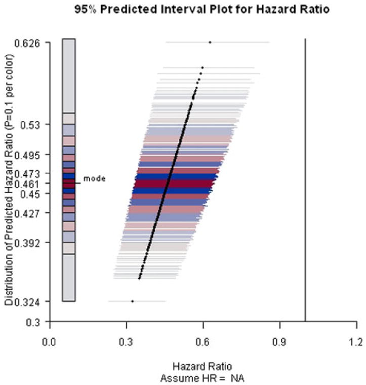
PIP for ACTG A320 study assuming current trend continues and the end-of-study time was two years after the first patient was randomized.

The construction of PIPS combines the ideas of forest plot (Lewis and Clarke 2001) and histogram by using the x-axis to indicate the values of the point estimates and the bounds of the intervals, and using the y-axis to indicate the degrees of concentration.

The high concentration regions close to the mode are highlighted by bright colors. With a vertical line representing the null value, the probability of being able to claim superiority at the end of the trial can be obtained directly from the plot as the percentage of predicted intervals which exclude the null value in favor of the alternative hypothesis. Similarly, we can also obtain the probability of being able to claim noninferiority at the end of the trial by adding a vertical line representing the noninferiority margin. Furthermore, the sampling variations in the predicted point estimates and in the length of the predicted intervals are explicitly presented in the plot. The gain of precision with trial continuation and the associated increase in sample size is reflected in the comparison of the length of the predicted intervals with the length of the current confidence interval. As the future data are generated under some user-specified parametric assumptions, we recommend conducting sensitivity analyses by varying the data-generating assumptions and/or the hypothetical off-study times under reasonable assumptions.

We recommend implementing our PIPS approach in combination with the repeated confidence intervals method, to provide more information and help the investigators make decisions. Our approach can be particularly useful in the following two scenarios. In the first scenario, suppose the prespecified stopping rule has been met at an interim look but the investigators are still concerned about whether the treatment effect could change over a longer follow-up period, our approach can easily help the investigators evaluate their concerns. If the results remain very promising even when the future data are generated under the null hypothesis, then the investigators should feel much more comfortable to stop the trial early and claim efficacy. In the second scenario, if the possibility of rejecting the null hypothesis at the end of the trial is fairly low even when the future data are generated under a very optimistic alternative hypothesis, then the investigators should consider stopping the trial early for futility to save resources and time. In addition, the information provided by our approach can be easily combined with other data such as safety data in the decision-making process.

4. Examples

4.1 ACTG A320

ACTG A320 was a randomized, double-blind, placebo-controlled trial evaluating the effect of adding a protease inhibitor (indinavir) to two nucleoside regimes (zidovudine and lamivudine) to treat HIV-1 infected patients with CD4 cell counts of no more than 200/μL (Hammer et al. 1997). The primary endpoint was time to the development of the acquired immunodeficiency syndrome (AIDS) or death. 1750 participants with no previous exposure to either lamivudine or protease inhibitors were expected to be recruited within 36 weeks, stratified according to CD4 cell count, and randomly assigned to one of the two treatment arms: (1) 600 mg of zidovudine and 300 mg of lamivudine daily (arm A), or (2) 600 mg of zidovudine, 300 mg of lamivudine, and 2,400 mg of indinavir daily (arm B). The plan was to follow all participants for an additional 48 weeks after the last patient was randomized. However, at the second review by the data and safety monitoring board (DSMB) on February 18, 1997, roughly one year after the first patient was randomized, a significant difference between the two treatment groups was observed. By then, 1,156 patients had entered the study. The estimated hazard ratio (HR) for the primary endpoint comparing arm B with arm A was 0.5 with a 95% confidence interval [0.33, 0.76] and a p-value < 0.001. Thus, the trial was stopped early for efficacy according to the trial design. The Kaplan–Meier curves by treatment were presented in Figure 1.

Figure 1.

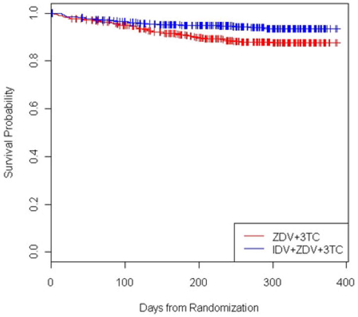
Kaplan–Meier curves for ACTG A320 study by treatment.

To evaluate the treatment effect over a longer followup period, we applied our approach to the data collected before the trial was stopped to predict the hazard ratio at a hypothetical end-of-study time, two years after the first patient was randomized. Future data between the second DSMB meeting and the hypothetical end-of-study time was simulated under three assumptions: the current trend continues (i.e., HR = NA), the null hypothesis (HR = 1) holds, and the alternative hypothesis (HR = 0.71) holds. The value of HR under the alternative hypothesis was obtained as the survival probabilities for the two treatment arms at the end of the study were expected to be 67% and 75.25%, respectively.

In all settings, we first fit two Weibull distributions to the interim data to obtain the estimates of the unknown parameters, which include two scale parameters and two shape parameters for the two treatment arms, respectively. Under the assumption that the current trend continues, the maximum likelihood estimates of the four unknown parameters were obtained. In the other two scenarios, the value of the hazard ratio was specified, which implies two constraints and thus decreases the degree of freedom in the parameter space to two. The parameter estimates were obtained by maximizing the likelihood under those constraints. After the parameter estimates were obtained, future data were simulated using the method introduced in Section 3.1 and the predicted point estimates and predicted intervals were obtained by fitting Cox proportion-hazards regression models.

Results are presented in Figures 2-4. When the current trend is assumed to continue, all predicted intervals exclude the null value. The conditional power increases slightly to about 95% under the alternative hypothesis that the hazard ratio equals 0.71. Even under the null hypothesis that there is no treatment effect on the survival functions, the conditional power is at least 60%, indicating that it is unlikely that the treatment effect will diminish with trial continuation and thus the decision to stop early for efficacy is justified.

Figure 4.

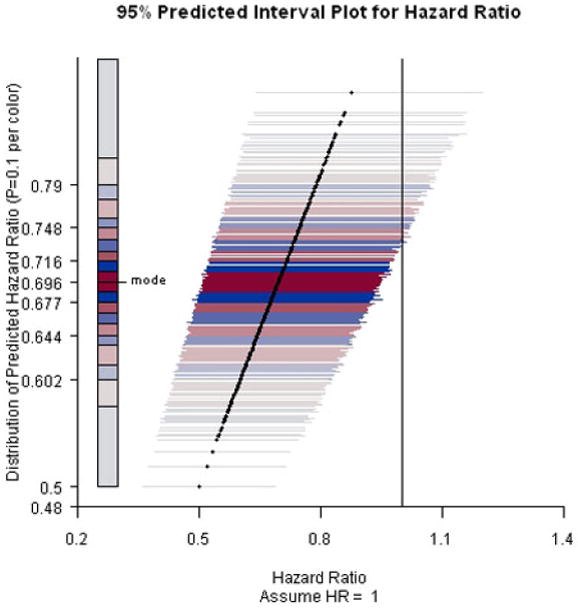
PIP for ACTG A320 study assuming hazard ratio equals 1 and the end-of-study time was two years after the first patient was randomized.

4.2 ACTG A5095

ACTG A5095 was a phase III, randomized, double-blind trial comparing three protease inhibitor-sparing regimens for the initial treatment of HIV infection (Gulick et al. 2004). The three regimens were: (1) ZDV+lamivudine+ABC (Arm A), (2) ZDV+lamivudine+EFV (Arm B), and (3) ZDV+lamivudine+ABC+EFV (Arm C). Arm A was discontinued for futility after an early interim analysis. Our interest is to compare Arms B and C with respect to the primary endpoint, time to virologic failure, defined as two consecutive HIV-1 RNA levels >200 copies/mL after 16 weeks on study. At a later interim analysis, the estimate of the hazard ratio for Arm C versus Arm B was 0.82 (95% CI = [0.60, 1.13]). The Kaplan–Meier curves by treatment are presented in Figure 5.

Figure 5.

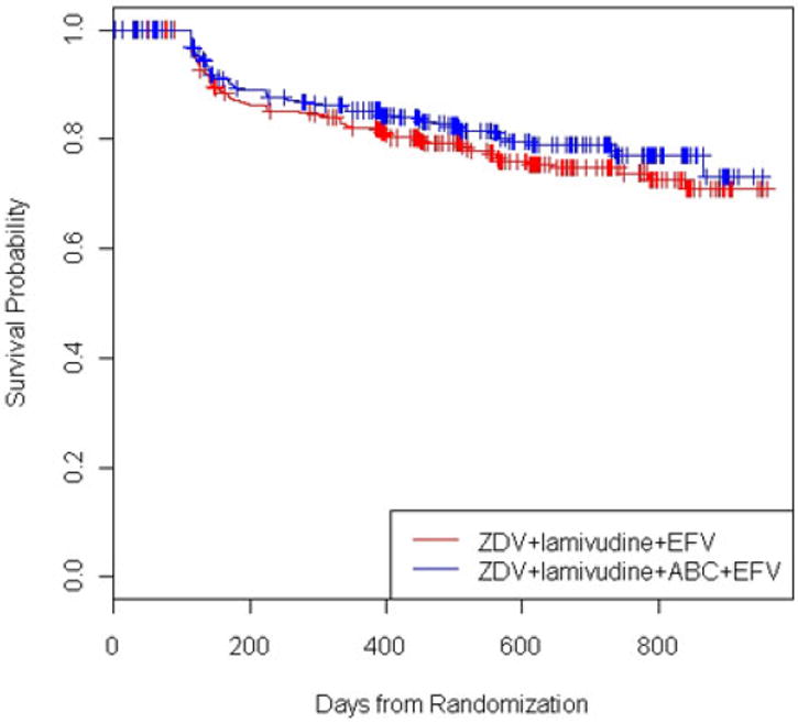
Kaplan–Meier curves for ACTG A5095 study by treatment.

The predicted intervals and the PIPS presented in Figures 6 and 7 were generated under the assumptions of the current trend continuing (i.e., HR = NA) and the alternative hypothesis (HR = 0.7) being valid, respectively. The end-of-study time was week 184 after the study initiation.

Figure 6.

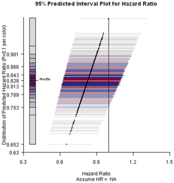
PIP for ACTG A5095 study predicting hazard ratio at week 184 assuming current trend continues.

Figure 7.

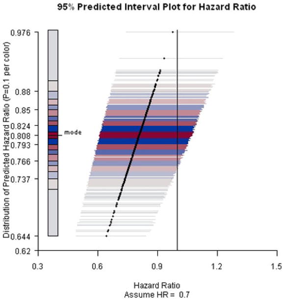
PIP for ACTG A5095 study predicting hazard ratio at week 184 assuming hazard ratio equals 0.7.

Assuming the current trend continues, the conditional power of rejecting the null hypothesis at the end of the trial is low (i.e., at least 80% of the predicted intervals fail to exclude the null value). The lengths of the predicted intervals are comparable to the length of the confidence interval, indicating little gain in precision with trial continuation.

Furthermore, even under the alternative hypothesis that the hazard ratio equals 0.7, the conditional power only increases approximately 5%–10%. Overall, the chance of rejecting the null hypothesis at the end of the trial is low. Notably, ACTG 5095 continued as planned after these interim analyses. The final analyses resulted in a hazard ratio estimate 0.95 and an insignificant 95% CI [0.72, 1.26].

5. Discussion

During the course of clinical trials, it is very important to consider all available information and provide investigators with a comprehensive evaluation of what have happened so far and what would happen if the investigators decide to continue or terminate the trial. The gains and losses need to be weighted carefully to make sure the best decision is made such that the study participants are well protected and the resources are efficiently used to benefit public health. The predicted intervals approach (Evans et al. 2007) and our predicted interval plots approach have been proposed to provide quantitative and flexible monitoring tools for clinical trials and aid in decision-making.

The advantages of using prediction and predicted intervals in data monitoring were discussed in detail by Evans et al. (2007) and have also been echoed in previous sections of this article. The predicted intervals are predictions of the confidence intervals for the parameter of interest at the final data analysis if the trial continues to the end. They are obtained through simulating the yet-to-be-observed data under reasonable assumptions. They provide information regarding effect size, are invariant to study design, and provide flexibility in the decision making process. As a graphical summary of the results from the prediction process, PIPS have made this idea more appealing and easier to implement. The sampling variations in the predicted point estimates and in the length of the predicted intervals are explicitly presented in the plot. The concentration of the predicted point estimates is displayed through their y-coordinates and then further emphasized by the color and brightness of the lines representing the corresponding predicted intervals. The gain of precision with trial continuation and the associated increase in sample size is reflected in the comparison of the length of the predicted intervals with the length of the current confidence interval. The conditional power of claiming superiority at the end of the trial can be obtained directly from the plot as the percentage of predicted intervals excluding the null value in favor of the alternative hypothesis. The probability of claiming noninferiority can be obtained similarly by adding a vertical line representing the noninferiority margin. Thus, nonstatistician members of Data Monitoring Committees can interpret the PIPs easily.

The yet-to-be-observed data are simulated under certain assumptions imposed by the investigators. Thus, sensitivity analysis is recommended. Both the data-generating assumptions and the hypothetical off-study times can be varied. The corresponding PIPS can be compared and then the probabilities of claiming superiority or noninferiority can be adequately evaluated and presented to the investigators together with other data such as safety data to help make the decisions.

An R program is available from the authors by request. The program conducts the data simulation under the user-specified assumptions, and then constructs the PIPS. The current version can be used for time-to-event endpoints only. In our future work, we expect to further improve that to include discrete and continuous endpoints.

Figure 3.

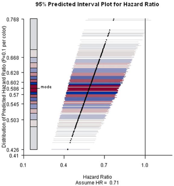
PIP for ACTG A320 study assuming hazard ratio equals 0.71 and the end-of-study time was two years after the first patient was randomized.

References

- Berntsen RF, Rasmussen K. Monitoring a Randomized Clinical Trial for Futility: The North-Norwegian Lidocaine Intervention Trial. Statistics in Medicine. 1991;10:405–412. doi: 10.1002/sim.4780100312. [DOI] [PubMed] [Google Scholar]
- Chang WH, Chuang-Stein C. Type I Error and Power in Trials with One Interim Futility Analysis. Pharmaceutical Statistics. 2004;3:51–59. [Google Scholar]
- Choi SC, Smith PJ, Becker DP. Early Decision in Clinical Trials when Treatment Differences Are Small. Controlled Clinical Trials. 1985;6:280–288. doi: 10.1016/0197-2456(85)90104-7. [DOI] [PubMed] [Google Scholar]
- EAST Users Manual. 2003 [Google Scholar]
- Evans SR, Li L, Wei LJ. Data Monitoring in Clinical Trials Using Prediction. Drug Information Journal. 2007;41:733–742. [Google Scholar]
- Gould AL, Pecore VJ. Group Sequential Methods for Clinical Trials allowing Early Acceptance of H0 and Incorporating Costs. Biometrika. 1982;69(1):75–80. [Google Scholar]
- Gulick RM, et al. Triple-Nucleoside Regimens versus Efavirenz-Containing Regimens from the Initial Treatment of HIV-1 Infection. The New England Journal of Medicine. 2004;350(18):1850–1861. doi: 10.1056/NEJMoa031772. [DOI] [PubMed] [Google Scholar]
- Harrington DP, Fleming TR, Green SJ. Procedures for Serial Testing in Censored Survival Data. In: Crowley J, Johnson RA, editors. Survival Analysis. Hayward, CA: Institute of Mathematical Statistics; 1982. pp. 269–286. [Google Scholar]
- Hammer SM, et al. A Controlled Trial of Two Nucleoside Analogues Plus Indinavir un Persons with Human Immunodeficiency Virus Infection and CD4 Cell Counts of 200 Per Cubic Millimeter or Less. The New England Journal of Medicine. 1997;337(11):725–730. doi: 10.1056/NEJM199709113371101. [DOI] [PubMed] [Google Scholar]
- Jennison C, Turnbull BW. Repeated Confidence Intervals for Group Sequential Clinical Trials. Controlled Clinical Trials. 1984;5:33–45. doi: 10.1016/0197-2456(84)90148-x. [DOI] [PubMed] [Google Scholar]
- Jennison C, Turnbull BW. Repeated Confidence Intervals for the Median Survival Time. Biometrika. 1985;72:619–625. [Google Scholar]
- Jennison C, Turnbull BW. Group Sequential Methods with Applications to Clinical Trials. Boca Raton, FL: CRC Press; 2000. [Google Scholar]
- Kim KKG, DeMets DL. Design and Analysis of Group Sequential Tests Based on the Type I Error Spending Rate Function. Biometrika. 1987;74:149–154. [Google Scholar]
- Lan KKG, DeMets DL. Discrete Sequential Boundaries for Clinical Trials. Biometrika. 1983;70(3):659–663. [Google Scholar]
- Lan KKG, Simon R, Halperin M. Stochastically Curtained Tests in Long-term Clinical Trials. Communications in Statistics—C. 1982;1:207–219. [Google Scholar]
- Lewis S, Clarke M. Forest Plots: Trying to See theWood and the Trees. British Medical Journal. 2001;322:1479–1480. doi: 10.1136/bmj.322.7300.1479. [DOI] [PMC free article] [PubMed] [Google Scholar]
- O’Brien PC, Fleming TR. A Multiple Testing Procedure for Clinical Trials. Biometrics. 1979;35:549–556. [PubMed] [Google Scholar]
- Pampallona S, Tsiatis AA. Group Sequential Designs for One-sided and Two-sided Hypothesis Testing with Provision for Early Stopping in Favor of the Null Hypothesis. Journal of Statistical Planning and Inference. 1994;42:19–35. [Google Scholar]
- Pampallona S, Tsiatis AA, Kim K. Interim Monitoring of Group Sequential Trials Using Spending Functions for the Type I and Type II Error Probabilities. Drug Information Journal. 2001;35:1113–1121. [Google Scholar]
- Pocock SJ. Group Sequential Methods in the Design and Analysis of Clinical Trials. Biometrika. 1977;64:191–199. [Google Scholar]
- Slud EV, Wei LJ. Two-Sample Repeated Significance Tests Based on the Modified Wilcoxon Statistic. Journal of the American Statistical Association. 1982;77:862–868. [Google Scholar]
- Tsiatis AA. Group Sequential Methods for Survival Analysis with Staggered Entry. In: Crowley J, Johnson RA, editors. Survival Analysis. Hayward, CA: Institute of Mathematical Statistics; 1982. pp. 257–268. [Google Scholar]
- Wang SK, Tsiatis AA. Approximately Optimal One-Parameter Boundaries for Group Sequential Trials. Biometrics. 1987;43:193–199. [PubMed] [Google Scholar]
- Wang SK, Tsiatis AA. The Design and Analysis of Sequential Clinical Trials. 2. New York: Halstead Press; 1997. [Google Scholar]
- Whitehead J, Stratton U. Group Sequential Clinical Trials with Triangular Continuation Regions. Biometrics. 1983;39:227–236. [PubMed] [Google Scholar]