Estimating Missing Heritability for Disease from Genome-wide Association Studies

Abstract

Genome-wide association studies are designed to discover SNPs that are associated with a complex trait. Employing strict significance thresholds when testing individual SNPs avoids false positives at the expense of increasing false negatives. Recently, we developed a method for quantitative traits that estimates the variation accounted for when fitting all SNPs simultaneously. Here we develop this method further for case-control studies. We use a linear mixed model for analysis of binary traits and transform the estimates to a liability scale by adjusting both for scale and for ascertainment of the case samples. We show by theory and simulation that the method is unbiased. We apply the method to data from the Wellcome Trust Case Control Consortium and show that a substantial proportion of variation in liability for Crohn disease, bipolar disorder, and type I diabetes is tagged by common SNPs.

Introduction

Heritability is a general and key population parameter that can help understand the genetic architecture of complex traits. It is usually defined as the proportion of total phenotypic variation that is due to additive genetic factors.¹ Methods of obtaining unbiased estimates of heritability from pedigree data are well established for continuous phenotypes, for example (restricted) maximum likelihood for linear mixed models (LMM).^2–5 For binary traits, such as disease, familial resemblance is usually parameterized on an unobserved continuous liability scale so that the heritability is independent of disease prevalence.⁶ With genome-wide genotype data, we can derive estimates of genetic variance tagged by the SNPs from samples of individuals who are unrelated in the conventional sense.⁷ Heritability estimated from pedigree data is not the same as the proportion of phenotypic variation explained by all SNPs because the former includes the contribution of all causal variants, whereas the latter only includes the contribution of causal variants that are in linkage disequilibrium (LD) with the genotyped SNPs.⁸

Genome-wide association studies (GWAS) have reported hundreds of SNPs that are robustly associated with one or more complex traits, including quantitative traits and common disease.⁹ Typically, the associated SNPs in total only explain a small proportion of the genetic variation in the population, and this observation has led to the perceived problem of “missing heritability.”^10,11 We have argued previously that the two most plausible explanations for these observations are that either the effect sizes at individual SNPs are so small that they do not reach genome-wide significance in GWAS or that causal variants are not in sufficient LD with SNPs on the commercial arrays to be detected by association.^7,12 For example, insufficient LD could arise if causal variants have lower minor allele frequency (MAF) than genotyped SNPs. To test these hypotheses, we recently developed a method to estimate the proportion of variance explained by all SNPs in GWAS for a quantitative trait.⁷ We showed that a substantial proportion of genetic variation for human height was associated with common SNPs. For complex diseases it would be very useful to apply the same estimation procedure to case-control GWAS data. However, there are three issues that need to be overcome to be able to estimate genetic variance for disease without bias and with computationally fast algorithms:

• (1)Scale. For quantitative traits the scale of measurement is the same as the scale on which heritability is expressed. For disease traits, the phenotypes (case-control status) are measured on the 0–1 scale, but heritability is most interpretable on a scale of liability.
• (2)Ascertainment. In case-control studies the proportion of cases is usually (much) larger than the prevalence in the population yet estimates of genetic variation are most interpretable if they are not biased by this ascertainment.
• (3)Quality control (QC) of SNPs. QC is more of a concern for case-control than quantitative GWAS. For quantitative traits, experimental or genotyping artifacts are unlikely to be correlated with the trait value. However, case and control sets are often collected independently so that experimental artifacts could make cases more similar to other cases and controls more similar to other controls. These artificial case-control differences could be partitioned as “heritability” in methods that utilize genome-wide similarity within and differences between cases and controls.

In the present study, we overcome all three problems and by using theory, simulations, and analysis of real data show that genetic variation in liability to disease that is in LD with common SNPs can be estimated from GWAS data. The purpose of this paper is to present these methods in detail. We demonstrate their application by using three of the data sets from the Wellcome Trust Case Control Consortium (WTCCC),¹³ Crohn disease, bipolar disorder, and type I diabetes. We show that a substantial proportion of variation in liability to these diseases is captured by common SNPs.

Material and Methods

We first revisit the concept of using marker data to estimate realized genetic relationships. Next we present the linear model between binary phenotype and genetic effects (this is the same model as used for continuous phenotypes) and use this model to estimate genetic variance. We then demonstrate the derivation of the classic relationship between additive genetic variance on the disease and liability scales that allows interpretation of genetic variance on the liability scale. For case-control studies, we adapt this relationship to account for ascertainment that generates a much higher proportion of cases in our analyzed sample than in the population. The new theory is general and applicable to any proportion of cases and controls in a case-control study. We apply these methods first to simulated data in which we can vary the disease prevalence and genetic variance explained by the SNPs. We then apply these methods to real GWAS data by focusing on stringent QC steps required to get meaningful results.

Theory on Random Variables

Throughout subsequent derivations, we repeatedly make use of a number of known results from statistical theory. For random variables x and y, their variances and covariance are defined as

$$\begin{array}{l}\text{var}\left(x\right)=\text{E}\left(x^2\right)-\text{E}{\left(x\right)}^2,\\ \text{var}\left(y\right)=\text{E}\left(y^2\right)-\text{E}{\left(y\right)}^2\end{array}$$ (Equation 1)

and

$$\text{cov}\left(x,y\right)=\text{E}\left(xy\right)-\text{E}\left(x\right)\text{E}\left(y\right)\text{.}$$ (Equation 2)

The bivariate regression of y on x has regression coefficient

$$\text{β}=\text{cov}\left(x,y\right)/\text{var}\left(x\right)\text{.}$$ (Equation 3)

If y follows a standard normal distribution with a truncation point at t, with t > 0, so that the fraction of y that is larger than t is K, then the mean value of y above the truncation point is

$$\text{E}\left(y|y>t\right)=\text{i}=z/K,$$ (Equation 4)

with z the height of the normal curve at point t.^2,3 The mean for y below the truncation point is

$$\text{E}\left(y|y<t\right)=-iK/\left(1-K\right).$$ (Equation 5)

The variance of y for values above and below the truncation point are [1 − i(i-t)] and [1 − itK/(1-K)(t + iK/(1 − K)], respectively.² It follows from the definition of the variance given above that

$$\text{E}\left(y^2|y>t\right)=\left[1+it\right]$$ (Equation 6)

and

$$\text{E}\left(y^2|y<t\right)=\left[1-itK/\left(1-K\right)\right].$$ (Equation 7)

Realized Relationships between Distant Individuals

We showed previously that it is possible to estimate realized relationships between unrelated (in a conventional sense) individuals from dense SNP data.⁷ A simple and logical method of estimating realized additive genetic relationships (${\widehat{A}}_{ij}$) between individual i and j is to use the products of genotype indicator coefficients between two individuals scaled by the heterozygosity for all L genotyped SNPs across the genome,⁷

$${\widehat{A}}_{ij}=\frac{1}{L}\sum _{i=1}^L\left(x_{il}-2p_l\right)\cdot \left(x_{jl}-2p_l\right)/\left(2p_l{q}_l\right)\left(i\ne j\right),$$ (Equation 8)

where x_il = 0, 1, or 2 according to whether individual i has genotype bb, Bb, or BB at locus l (alleles are arbitrarily called b or B), p (q) is allele frequency of B (b), and 2p is the mean of x_l. As in Yang et al.,⁷ we use the current population as the base (reference) population when estimating relatedness from SNP data so that E(x) = 2p in the current population. This implies that the average pairwise relatedness is zero and that some pairs of individuals are less related to each other than the average in the population, leading to negative estimates. Relatedness in this definition is not a probability (as in the classical definition of identity-by-descent) but a correlation of additive genetic values.^2,14 The estimate of relatedness for an individual with him/herself (the diagonal of the matrix) has a slightly different form to the off-diagonals to minimize sampling variation,⁷

$${\widehat{A}}_{ii}=1+\frac{1}{L}\sum _{i=1}^L\left(x_{il}^2-\left(1+2p_l\right)x_{il}+2p_l^2\right)/\left(2p_l{q}_l\right).$$

Linear Mixed Model

In a model for analyzing disease, the observations (unaffected or affected) can be expressed as a linear function of the sum of the additive effects due to SNPs associated with causal variants and residual effects. The linear model can be written as

$$\mathbf{y}=\mu {\mathbf{1}}_{\mathbf{N}}+\mathbf{u}+\mathbf{e}$$ (Equation 9)

where y is a vector of 0, 1 observations of disease status for N individuals, μ is the overall mean, 1_N is a vector of N ones, u is a vector of random additive genetic effects from aggregate SNP information, and e is a vector of residuals. The variance structure of phenotypic observations is written as $\mathbf{V}=\mathbf{A}{\sigma }_u^2+\mathbf{I}{\sigma }_e^2$, where A is the realized relationship matrix estimated from SNP data, I is an identity matrix, ${\sigma }_u^2$ is polygenic additive genetic variance explained by the SNPs, and ${\sigma }_e^2$ is error variance; these variances are on the observed 0–1 scale. Therefore, the heritability on the observed scale is $h_o^2={\sigma }_u^2/\left({\sigma }_u^2+{\sigma }_e^2\right)$, the ratio of total phenotypic variance on that scale that is due to additive genetic effects. The variance components are estimated via residual maximum likelihood (REML) analysis.^4,15,16

Liability Threshold Model

One can model the relationship between observations on the observed risk scale and liabilities on the unobserved continuous scale by using a probit transformation to generate the classical liability threshold model⁶ (Figure 1). Liability of disease is assumed to be the sum of environmental and additive genetic components from independent normal distributions. The advantages of working on the scale of liability are that population parameters such as variance components and heritability are independent of prevalence and can therefore be compared across traits or populations and that statistical methods developed for quantitative traits can be applied to the trait liability.^2,6 The model can be written as

$$\mathbf{l}=\mu {\mathbf{1}}_{\mathbf{N}}+\mathbf{g}+\mathbf{e}$$ (Equation 10)

where l is a vector of liability phenotypes that are distributed as N(0, 1), g is a vector of random additive genetic effects on the liability scale that are distributed N(0, ${\sigma }_g^2$), and other terms are the same as in the linear model but on the liability scale. We note that the mean of the distribution of liability is zero (μ = 0) when there is no ascertainment. Therefore, because the total phenotypic variance on the scale of liability is per definition equal to 1 and the heritability is defined as the genetic variance as a proportion of total variance, the heritability on the liability scale is $h_l^2={\sigma }_g^2$. In the liability threshold model, all affected individuals have liability phenotypes exceeding a certain threshold value t (Figure 1). The population prevalence is K = E(y). Applying the properties of truncated normal distributions^2,17, Equations 4 and 5 give the mean liability

$$i=E\left(l|y=1\right)=z/K\text{for}\text{cases}\text{and}$$ (Equation 11)

$$i_2=E\left(l|y=0\right)=-z/\left(1-K\right)=-iK/\left(1-K\right)\text{for}\text{controls},$$ (Equation 12)

and, Equations 6 and 7 then give the squared mean liability as

$$E\left(l^2|y=1\right)=1+it\text{for}\text{cases}\text{and}$$ (Equation 13)

$$E\left(l^2|y=0\right)=1+i_{2}t\text{for}\text{controls}\text{.}$$ (Equation 14)

Figure 1.

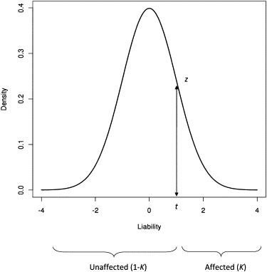
The Liability Threshold Model for a Disease Prevalence of K

An underlying continuous random variable determines disease status. If liability exceeds the threshold t, then individuals are affected.

By using Equations 2, 11, and 12, we can derive the covariance between y (unaffected/affected status) and l (liability) as

$$\mathrm{cov}\left(y,l\right)=E\left(y\cdot l\right)-E\left(y\right)E\left(l\right)=K1i+\left(1-K\right)0i_2=Ki=z,$$

where z is the height of the standard normal probability density function at the truncation threshold t. The above derivations describe the relationship between the phenotypes on the two scales, but what we are interested in is the relationship between genetic values on those scales. Following Dempster and Lerner,¹⁸ we determine the genetic value on the observed 0–1 risk scale for an individual (u), defined in Equation 9, as

$$u=c+bg=c+zg,$$ (Equation 15)

where c is a constant.

The linear regression coefficient that links the two scales is derived from the regression of the phenotype on the observed scale (y) on the additive genetic effect on the scale of liability (g), and equals the covariance of y and g divided by the variance of g (Equation 3),

$$b=\mathrm{cov}\left(y,g\right)/{\sigma }_g^2=\left[E\left(y\cdot g\right)-E\left(y\right)E\left(g\right)\right]/h_l^2=Ki{h}_l^2/h_l^2=z.$$ (Equation 16)

Finally, the heritability on the observed scale is the genetic variance on the observed scale, ${\sigma }_u^2=\mathrm{var}\left(zg\right)=z^2{\sigma }_g^2$ from Equation 15, as a proportion of the total variance of 0–1 observations, which is the Bernoulli distribution variance K(1 − K) and can be written as

$$h_o^2={\sigma }_u^2/\left[K\left(1-K\right)\right]={\sigma }_g^2{\left[\mathrm{cov}\left(y,g\right)/{\sigma }_g^2\right]}^2/\left[K\left(1-K\right)\right]={\sigma }_g^2{b}^2/\left[K\left(1-K\right)\right]=h_l^2{z}^2/\left[K\left(1-K\right)\right].$$

This can be rearranged to transform the heritability on the observed scale to that on the liability scale as

$$h_l^2=h_o^{2}K\left(1-K\right)/z^2.$$ (Equation 17)

This linear transformation was derived by Alan Robertson in the Appendix of Dempster and Lerner.¹⁸ When applied to estimates of genetic variation on the observed scale derived from family data, this transformation can give biased estimates on the liability scale because the genetic variation estimable from close relatives contains both additive and nonadditive variance.^18,19 However, when the genetic variance is estimated from distant relatives, the nonadditive genetic component of the variance is small relative to the additive component, and so the Robertson transformation provides a good approximation. Because we are using genetic relationships between “unrelated” individuals, the Robertson approximation is valid in samples without ascertainment. However, in order to obtain a relationship between the estimates of heritability on the two scales, we need to account for the inflated proportion of cases in case-control designs.

Ascertainment-Corrected Transformation to the Estimated Variance in a Case-Control Study to Estimate $h_l^2$

We consider the same liability model when the proportions of cases and controls are not a random sample from the population (Figure 2). The mean and variance for case and control disease status (y_cc), disease liability (l_cc), and genetic liability (g_cc) following quantitative genetic theory² are

$$E\left(y_{cc}\right)=P,\text{which is the proportion of cases in the sample}\left(\text{usually}1/2\right),$$

$$\text{var}\left(y_{cc}\right)=P\left(1-P\right),\text{which is the phenotypic variance on the}\text{observed scale in the case-control sample, and}$$

$$E\left(l_{cc}\right)=Pi+\left(1-P\right)i_2=i\lambda ,\text{where}\text{we}\text{define}\lambda =\left(P-K\right)/\left(1-K\right).$$

Figure 2.

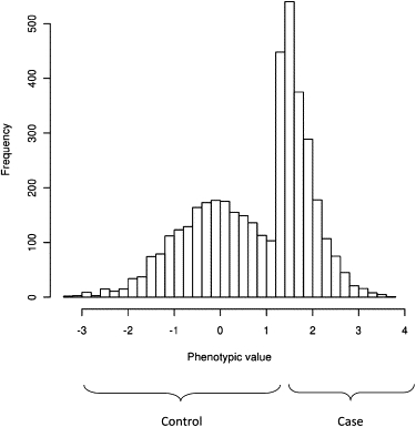
The Distribution of Liability When Cases Are Oversampled as in a Case-Control Study

Using Equations 1, 13, and 14 then gives,

$$\mathrm{var}\left(l_{cc}\right)={\sigma }_{l_{cc}}^2=E\left(l_{cc}^2\right)-E{\left(l_{cc}\right)}^2=P\left(1+it\right)+\left(1-P\right)\left(1+i_{2}t\right)-i^2{\lambda }^2$$

$$=1+Pit-\left(1-P\right)tiK/\left(1-K\right)-i^2{\lambda }^2=1+i\lambda \left(t-i\lambda \right)=1+\theta ,$$ (Equation 18)

where $\theta =i\lambda \left(t-i\lambda \right)$, that is, the variance of liability is greater than 1 in a case-control study because individuals from the tails of the distribution of liability have been selected. Because cases (and controls) are ascertained on the observed phenotypic scale, the mean of genetic liability depends on the mean liability phenotype of the cases and the heritability of liability,

$$E\left(g_{cc}\right)=h_l^{2}E\left(l_{cc}\right)=h_l^2\left[Pi+\left(1-P\right)i_2\right]=h_l^{2}i\lambda .$$

By using Equations 1, 13, 14, and 18 with the heritability of liability, we can derive the variance for genetic liability as

$$\mathrm{var}\left(g_{cc}\right)={\sigma }_{g_{cc}}^2=E\left(g_{cc}^2\right)-E{\left(g_{cc}\right)}^2=h_l^{2}E\left(l_{cc}^2\right)-{\left[h_l^{2}E\left(l_{cc}\right)\right]}^2$$

$$=h_l^2\left[P\left(1+it\right)+\left(1-P\right)\left(1+i_{2}t\right)\right]-h_l^4{i}^2{\lambda }^2=h_l^2\left(1+h_l^2\theta \right).$$

The expression for ${\sigma }_{g_{cc}}^2$ was previously derived in the context of estimation of the accuracy of predicting the genetic risk of disease from case-control studies.²⁰ As for the situation of no ascertainment, we are interested in the regression of phenotype on the observed risk scale on genetic liability in the case-control study,

$$b_{cc}=\mathrm{cov}\left(y_{cc},g_{cc}\right)/\mathrm{var}\left(g_{cc}\right)=\left[E\left(y_{cc}\cdot g_{cc}\right)-E\left(y_{cc}\right)E\left(g_{cc}\right)\right]/\mathrm{var}\left(g_{cc}\right)=\left[h_l^{2}iP-h_l^{2}i\lambda P\right]/{\sigma }_{g_{cc}}^2=\left[P{h}_l^{2}i\left(1-\lambda \right)\right]/{\sigma }_{g_{cc}}^2=z\frac{P\left(1-P\right)}{K\left(1-K\right)}\frac{{\sigma }_g^2}{{\sigma }_{g_{cc}}^2}.$$ (Equation 19)

The term $\frac{P\left(1-P\right)}{K\left(1-K\right)}\frac{{\sigma }_g^2}{{\sigma }_{g_{cc}}^2}$ quantifies the change of the regression coefficient due to ascertainment in a regression of phenotype on the observed risk scale onto genetic factors on the scale of liability. In the absence of ascertainment (P = K), this term is 1.

According to Equation 15, the genetic value on the observed scale (u_cc) for an individual in a case-control study is

$$u_{cc}=c+b_{cc}{g}_{cc}=c+z\frac{P\left(1-P\right)}{K\left(1-K\right)}\frac{{\sigma }_g^2}{{\sigma }_{g_{cc}}^2}{g}_{cc},$$

and

$${\sigma }_{u_{cc}}^2=b_{cc}^2{\sigma }_{g_{cc}}^2={\left[z\frac{P\left(1-P\right)}{K\left(1-K\right)}\frac{{\sigma }_g^2}{{\sigma }_{g_{cc}}^2}\right]}^2{\sigma }_{g_{cc}}^2={\left[z\frac{P\left(1-P\right)}{K\left(1-K\right)}\right]}^2\frac{{\sigma }_g^2}{{\sigma }_{g_{cc}}^2}{\sigma }_g^2.$$ (Equation 20)

We note that u_cc is a least-squares estimate of the genetic value on the observed scale. When residuals are normally distributed, the least-square estimate is the same as the (residual) maximum-likelihood estimate. However, normality of liability is violated in a case-control study. The previous section describes the theoretical relationships between parameters on different scales in the presence of ascertainment. In practice, we do not observe parameters directly but estimate them. We now consider the relationship between the parameters and their estimates when maximum likelihood is used to estimate the variance components.

The estimated genetic variance on the observed scale from REML analysis (Equation 9) is based on 0–1 observations and the covariance structure among samples. Without ascertainment, the mean of estimated genetic values on the observed scale can be derived from Equations 11, 12, 15, and 16 as $E\left(\widehat{u}|y=1\right)=zi{\sigma }_g^2$ for cases and $E\left(\widehat{u}|y=0\right)=z{i}_2{\sigma }_g^2$ for controls. When samples are ascertained, the mean of the estimated genetic values is

$$E\left({\widehat{u}}_{cc}|y_{cc}=1\right)=\frac{P}{K}\frac{\left(1-P\right)}{\left(1-K\right)}\frac{\left(1-P\right)}{\left(1-K\right)}E\left(\widehat{u}|y=1\right)\text{for}\text{cases}$$ (Equation 21)

and

$$E\left({\widehat{u}}_{cc}|y_{cc}=0\right)=\frac{P}{K}\frac{\left(1-P\right)}{\left(1-K\right)}\frac{P}{K}E\left(\widehat{u}|y=0\right)\text{for}\text{controls},$$

where the term $\frac{P}{K}\frac{\left(1-P\right)}{\left(1-K\right)}$ is due to the increased proportion of cases and the decreased proportion of controls, that is, in an ascertained case-control study, the mean genetic liability for cases can be transformed to that on the observed scale by $b_{cc}{i}^{\ast }{\sigma }_{g_{cc}}^2=\frac{P}{K}\frac{\left(1-P\right)}{\left(1-K\right)}z{i}^{\ast }{\sigma }_g^2$ and $b_{cc}{i}_2^{\ast }{\sigma }_{g_{cc}}^2=\frac{P}{K}\frac{\left(1-P\right)}{\left(1-K\right)}z{i}_2^{\ast }{\sigma }_g^2$ from Equations 11, 12, 15, and 19 and $i^{\ast }=i\frac{\left(1-P\right)}{\left(1-K\right)}$ and $i_2^{\ast }=i_2\frac{P}{K}$, which is derived as follows. According to Equation 17, $h_l^2=h_o^{2}K\left(1-K\right)/z^2={\widehat{h}}_{o_{cc}}^{2}P\left(1-P\right)/{\widehat{z}}_{cc}^2$, where ${\widehat{h}}_{o_{cc}}^2$ is estimated heritability on the liability scale in an ascertained case-control study and ${\widehat{z}}_{cc}^2$ is a squared regression coefficient that transforms the estimate of genetic factors on the observed risk scale to that on the liability scale. This expression can be written as $\frac{{\sigma }_u^2}{K\left(1-K\right)}\frac{1}{z}\frac{K\left(1-K\right)}{z}=\frac{{\widehat{\sigma }}_{u_{cc}}^2}{P\left(1-P\right)}\frac{1}{{\widehat{z}}_{cc}}\frac{P\left(1-P\right)}{{\widehat{z}}_{cc}}$. But from Equations 17, 19, and 20, the terms $\frac{{\sigma }_u^2}{K\left(1-K\right)}\frac{1}{z}$ on the left-hand side and $\frac{{\widehat{\sigma }}_{u_{cc}}^2}{P\left(1-P\right)}\frac{1}{{\widehat{z}}_{cc}}$ on the right-hand side are the same. Therefore, $\frac{K\left(1-K\right)}{z}=\frac{P\left(1-P\right)}{{\widehat{z}}_{cc}}$ results in the expressions $i^{\ast }=\frac{{\widehat{z}}_{cc}}{P}=i\frac{\left(1-P\right)}{\left(1-K\right)}$ and $i_2^{\ast }=-\frac{{\widehat{z}}_{cc}}{\left(1-P\right)}=i_2\frac{P}{K}$ that were given above. The REML estimate of the genetic variance (${\widehat{\sigma }}_u^2$ or ${\widehat{\sigma }}_{u_{cc}}^2$) is the covariance between observations and the unbiased estimate of the genetic values ($\widehat{u}$ or ${\widehat{u}}_{cc}$) with a normality assumption, that is, the regression of phenotype on predictor has a slope of 1, $\mathrm{cov}\left(y,\widehat{u}\right)/{\widehat{\sigma }}_u^2=1$ or $\mathrm{cov}\left(y_{cc},{\widehat{u}}_{cc}\right)/{\widehat{\sigma }}_{u_{cc}}^2=1$. Therefore,

$${\widehat{\sigma }}_u^2=\mathrm{cov}\left(y,\widehat{u}\right)=E\left(y\cdot \widehat{u}\right)-E\left(y\right)E\left(\widehat{u}\right)=E\left(y\cdot \widehat{u}\right)=E\left(\widehat{u}|y=1\right)\cdot K$$ (Equation 22)

and

$${\widehat{\sigma }}_{u_{cc}}^2=\mathrm{cov}\left(y_{cc},{\widehat{u}}_{cc}\right)=E\left(y_{cc}\cdot {\widehat{u}}_{cc}\right)-E\left(y_{cc}\right)E\left({\widehat{u}}_{cc}\right)=E\left(y_{cc}\cdot {\widehat{u}}_{cc}\right)=E\left({\widehat{u}}_{cc}|y_{cc}=1\right)\cdot P.$$

from Equations 21 and 22 and ${\widehat{\sigma }}_u^2=z^2{\widehat{\sigma }}_g^2$ from Equation 15 give us

$${\widehat{\sigma }}_{u_{cc}}^2={\left[\frac{P}{K}\frac{\left(1-P\right)}{\left(1-K\right)}\right]}^2{\widehat{\sigma }}_u^2={\left[z\frac{P}{K}\frac{\left(1-P\right)}{\left(1-K\right)}\right]}^2{\widehat{\sigma }}_g^2.$$

We note that in an ascertained case-control study, the REML estimate is larger than the least-square estimator (Equation 20) by a factor ${\sigma }_{g_{cc}}^2/{\sigma }_g^2$, i.e., ${\widehat{\sigma }}_{u_{cc}}^2=\left({\sigma }_{g_{cc}}^2/{\sigma }_g^2\right){\sigma }_{u_{cc}}^2$. This difference is due to the normality assumption in REML. Therefore,

$$h_l^2={\sigma }_g^2={\widehat{\sigma }}_{u_{cc}}^2{\left[\frac{1}{z}\frac{K\left(1-K\right)}{P\left(1-P\right)}\right]}^2={\widehat{h}}_{o_{cc}}^2\frac{K\left(1-K\right)}{z^2}\frac{K\left(1-K\right)}{P\left(1-P\right)}.$$ (Equation 23)

In the absence of ascertainment (P = K), this equation reduces to Equation 17, hence adjusting for ascertainment when variance components are estimated by maximum likelihood leads to a generalization of the classical Robertson transformation. Equation 23 shows the transformation that needs to be applied to the SNP-attributable variance estimated from Equation 9 to provide an estimate of the liability variance in the total population explained by the SNPs. The sampling variance of estimated heritability on the liability scale transformed from that on the observed scale can be derived with a Taylor series expansion,

$$\mathrm{var}\left(h_l^2\right)\sim {\left[\frac{d\left(h_l^2\right)}{d\left(h_{o_{cc}}^2\right)}\right]}^2\mathrm{var}\left(h_{o_{cc}}^2\right)={\left[\frac{K\left(1-K\right)}{z^2}\frac{K\left(1-K\right)}{P\left(1-P\right)}\right]}^2\mathrm{var}\left(h_{o_{cc}}^2\right).$$ (Equation 24)

With extreme ascertainment, for example, K < 0.01 and P = 0.5, a high heritability on the liability scale transforms to a greater genetic than phenotypic variance on the observed scale according to Equation 23. This is not a problem for the estimation of the genetic variance. When using REML or ML for estimation, it is possible to maximize the likelihood for the genetic variance on the observed scale even if it is larger than the observed phenotypic variance on that scale. Therefore, we can correctly estimate the heritability on the liability scale even with extreme K and high heritability on the liability scale.

In summary, in practice we can estimate the variance explained on the 0–1 risk scale in a case-control design by using a LMM and transform both the estimate and its standard error to the scale of liability while adjusting simultaneously for ascertainment.

Simulated Data

To test the estimation of genetic variance on the liability scale from ascertained case-control data, we performed a simulation study. For each simulation replicate we generated 5000 cases and 5000 controls. To achieve a low level of relatedness, we simulated individuals in independent batches of 100 with genetic values (g) drawn from a multivariate normal distribution given a 100 × 100 covariance matrix (the mvrnorm function in the R package was used²¹). Elements of the covariance matrix were 0.05 ${\sigma }_g^2$ for off-diagonals and ${\sigma }_g^2$ for diagonals. Environmental effects were sampled from a normal distribution with a mean of zero and a variance of ${\sigma }_e^2$, with ${\sigma }_e^2$ chosen such that the desired heritability of liability was obtained. As in equation (10), liability, l, for each individual consists of genetic effects, g, and residuals, e, on the liability scale; that is, l = g + e. Disease status for each individual was determined by comparing l with the threshold of liability determined by the population prevalence. For example, for K = 0.1, individuals were assigned to be a case if l > 1.282σ_l. From each batch, all cases and an equal number of randomly selected controls contributed to the case-control sample. We continued simulating batches of individuals until the desired sample size of 5000 cases and 5000 controls was achieved. The pairwise relationships between individuals in the case-control sample were 0.05 if they both came from the same set and zero otherwise.

For the analysis of the simulated data, we used the LMM Equation 9 with the transformation that was derived in Equation 23. Simulations were performed for K=0.001, 0.01, 0.10, 0.20, and 0.5, and the case-control samples were generated either without ascertainment (P = K) or with ascertainment (P > K), where each set of 100 individuals contributed approximately the same number of cases and controls. A range of values of heritability on the liability scale, $h_l^2$, were tested. One hundred simulation replicates were conducted for each scenario.

Real Data

We applied our estimation method to WTCCC GWAS data,¹³ genotyped on the Affymetrix 5.0 platform. QC is important with real data because artificial allele frequency differences between cases and controls will generate a spurious “heritability.” As a test of the robustness of the method, we first used the two independent control samples and pretended they formed a case-control study. One of the two control groups was treated as a case group, and the other was treated as a control group in the analysis. Subsequently, we estimated genetic variance explained by all SNPs by analyzing case samples for Crohn disease, bipolar disorder, and type I diabetes along with the combined data set of the two control samples. We fit the first 20 principal components as covariates in the LMM (Equation 9) to correct for possible population structure.²²

For each data set, a standard QC procedure was performed. SNPs with MAFs <0.01 and missing rates >0.05 were excluded as were individuals with missing rates >0.01. Because small errors for each SNP can be accumulated to give incorrect estimates for genetic variance, additional QC steps were extremely stringent. We excluded SNPs whose p values were <0.05 for the Hardy-Weinberg (H-W) equilibrium test and for missingness-difference between cases and controls. We also applied a two-locus test based on the difference in the test statistic of association between single SNPs and pairs of adjacent SNPs.²³ Sex chromosomes were excluded from the analysis. To keep individuals who were only distantly related, both individuals from a pair with an estimated relationship >0.05 were excluded; to benchmark this threshold, relationships approximately closer than second cousins were removed. After the stringent QC process, the number of samples and SNPs used for estimating genetic variance were 2599 individuals (1395 cases and 1204 controls) and 309,040 SNPs for the control-control contrast study, 3833 individuals (1504 cases and 2329 controls) and 322,142 SNPs for Crohn disease, 3880 individuals (1433 cases and 2447 controls) and 321,605 SNPs for bipolar disorder, and 4063 individuals (1640 cases and 2423 controls) and 318,044 SNPs for type I diabetes.

To investigate the robustness of our variance estimates, we also considered more stringent threshold values for SNP missing rates (fewer than 20, 7, or 4 genotypes per SNP) and MAF (>0.05). To benchmark these thresholds, we note that a SNP missing rate of 0.05 is approximately equal to a maximum of 200 missing genotypes per SNP.

Each QC step was designed to remove potential artifacts from contributing to the estimate of genetic variance. However, each step also reduces the number of SNPs used for estimation of the genetic variance. As the number of SNPs decreases, the LD between genotyped and causal variants also decreases, and so estimates of genetic variance are expected to decrease. To determine whether any observed reduction in estimated genetic variance was a consequence of the reduced number of SNPs rather than the QC criteria per se, we adjusted the estimate of variance to take account of imperfect LD between the genotyped SNPs. That is, we adjusted the estimate because pairwise relatedness is estimated with error. We described previously how this adjustment was made.⁷ Subsequent to the adjustment for using a finite number of SNPs, we used the transformation in Equation 23 to obtain an estimate on the liability scale that takes account of ascertainment of cases in a case-control sample. In the transformation, we assumed a population prevalence of 0.1%, 0.5%, and 0.5% for Crohn disease, bipolar disorder, and type I diabetes, respectively.^13,24–26 Hence, our procedure was as follows: (1) REML analysis of 0–1 data using relatedness estimated from SNP data,¹⁶ (2) adjustment for the number of SNP used to construct relationships, and (3) adjustment for scale and ascertainment.

Results

Simulations

We used REML to estimate heritability on the observed scale, and we transformed estimates to the liability scale with the ascertainment correction from Equation 23. When simulated data with K = P = 0.5 (no ascertainment) were used, the estimated heritabilities on the liability scale were unbiased and close to the true values, as expected (Table 1). When ascertained case-control studies were used, the estimates were largely unbiased although a slight overestimation was observed for an extreme value of K = 0.001 (Table 1).

Table 1.

Simulation Results: Estimated Heritability on the Liability Scale and Empirical Standard Error over Replicates

Prevalence of Disease in the Population (K)	Heritability of Liability
	0.1	0.3	0.5	0.7	0.9
K = 0.5	0.09 (0.006)	0.28 (0.010)	0.51 (0.013)	0.70 (0.016)	0.90 (0.016)
K = 0.2	0.10 (0.007)	0.31 (0.009)	0.49 (0.011)	0.71 (0.012)	0.91 (0.013)
K = 0.1	0.11 (0.007)	0.30 (0.009)	0.49 (0.009)	0.71 (0.012)	0.89 (0.012)
K = 0.01	0.11 (0.009)	0.30 (0.011)	0.49 (0.012)	0.70 (0.013)	0.90 (0.012)
K = 0.001	0.17 (0.020)	0.31 (0.020)	0.56 (0.021)	0.75 (0.021)	0.94 (0.022)

In all examples the proportion of cases in the case-control sample was p = 0.5. Sample size was 10,000 (5000 cases, 5000 controls) for all situations. The number of replicates was 100.

Estimated Genetic Variance from the WTCCC Data after Stringent QC

In preliminary analyses, we recognized the importance of imposing stringent QC on H-W equilibrium, on differential missingness between cases and controls, and on a two-locus QC test (see Figures S1–S3, available online). Genotyping conducted on other platforms might not require this level of stringency. We conducted a range of additional tests and checks to ensure the validity of our results (see Discussion and Supplemental Data).

Control-Control Contrast Study

Estimates for genetic variance between the two control groups were not significantly different from zero, as expected (Table 2). The estimate and its likelihood ratio gradually decreased when the threshold for the SNP missing rate decreased. When SNPs with an MAF > 0.01 and missing <4 genotypes/SNP were used, the estimate was 0.06 (SE = 0.11). When SNPs with an MAF > 0.05 were used, the decreasing patterns of the estimates and their likelihood ratios were very similar to those of SNPs with an MAF > 0.01. The estimated values observed when SNPs with an MAF > 0.05 were used were slightly higher than those with an MAF > 0.01 although the difference was small. These results suggest that our QC procedure was stringent enough to allow robust estimates of genetic variation, that is, the likelihood ratio was already not significant for a SNP genotype missingness of up to 200.

Table 2.

Estimated Genetic Variance in the Observed Scale Explained by All SNPs for Two Control Samples in the WTCCC Data

Thresholda	No. SNPb	Estimatec(SE)	LRd	p valuee
MAF > 0.01
200	309,040	0.17 (0.11)	2.29	0.07
20	297,198	0.13 (0.11)	1.31	0.13
7	266,534	0.08 (0.11)	0.59	0.22
4	226,165	0.06 (0.11)	0.29	0.30
MAF > 0.05
200	278,564	0.19 (0.11)	3.42	0.03
20	267,043	0.16 (0.10)	2.33	0.06
7	239,614	0.12 (0.10)	1.33	0.12
4	203,698	0.09 (0.10)	0.92	0.17

^aExcluding SNPs with more than the listed number of missing genotypes. Two hundred missing genotypes are approximately equal to a missingness rate of 5% (depending on sample size).

^bAfter filtering on the basis of SNP missing rate.

^cEstimate of genetic variance proportional to the total phenotypic variance on the observed scale.

^dLikelihood-ratio test statistic.

^ep values were calculated assuming that the LR is distributed as a 50:50 mixture of zero and ${\chi }_1^2$ under the null hypothesis.

Crohn Disease

We investigated the impact of SNP missingness on the estimates of variance explained by SNPs for Crohn disease. While the threshold for missingness becomes more stringent, the number of SNPs reduces from ∼322,000 to ∼196,000 when MAF > 0.01 (Table 3). While this happens, the raw proportion of variance estimate drops from 0.56 to 0.50. Part of this decline is due to the reduced number of SNPs used rather than artifacts of genotype missingness. After we adjust for the number of SNPs, the proportion of variance estimate drops from 0.64 to 0.61 but reaches a plateau at that value (Table 3, Adjusted column). Therefore we conclude that there is no need to make the missing threshold more stringent than 20. On the liability scale, the heritability estimate (i.e., the variance in liability explained by the SNPs) is 0.22 (SE = 0.04), which is much higher than that explained by genome-wide significant SNPs.²⁷ Similar results are obtained if the SNPs with MAF >0.05 are used (Table 3). This indicates that common SNPs (MAF > 0.05) are in substantial LD with casual variants for Crohn disease.

Table 3.

Estimated Genetic Variance on the Observed and Liability Scale Explained by All SNPs for Crohn Disease in WTCCC Data

Thresholda	No. SNPb	Estimatec(SE)	LR	Adjustedd(SE)	Transformede(SE)
MAF > 0.01
200	322,142	0.56 (0.07)	63.16	0.64 (0.08)	0.24 (0.03)
20	294,850	0.53 (0.07)	57.48	0.61 (0.08)	0.22 (0.03)
7	248,791	0.52 (0.07)	57.30	0.61 (0.08)	0.22 (0.03)
4	195,977	0.50 (0.07)	54.94	0.60 (0.08)	0.22 (0.03)
MAF > 0.05
200	293,269	0.56 (0.07)	69.00	0.63 (0.08)	0.23 (0.03)
20	266,843	0.53 (0.07)	63.27	0.60 (0.08)	0.22 (0.03)
7	225,043	0.52 (0.07)	63.94	0.60 (0.08)	0.22 (0.03)
4	177,615	0.50 (0.07)	62.14	0.60 (0.08)	0.22 (0.03)

^aExcluding SNPs with more than the listed number of missing genotypes.

^bAfter filtering on the basis of SNP missing rate.

^cEstimate of genetic variance proportional to the total phenotypic variance on the observed scale.

^dEstimate adjusted for reduced number of SNPs.

^eTransformed genetic variance proportional to the total phenotypic variance on the liability scale under the assumption that the population prevalence is 0.1%, the heritability on the liability scale explained by the SNPs.

Bipolar Disorder

For bipolar disorder, we found that we needed a slightly more stringent threshold for SNP missingness than for Crohn disease. When we excluded SNPs with an MAF < 0.01 and missing rate >200, the heritability estimate on the liability scale was 0.4 (Table 4). The estimates gradually decreased and became stable after we excluded SNPs with more than seven missing genotypes. The estimated value was 0.38 (SE = 0.04). When we used SNPs with an MAF > 0.05, the decreasing pattern of the estimate and its likelihood was similar to that with an MAF > 0.01, and the values were slightly lower than those with an MAF > 0.01. When we used SNPs with missingness of <7 or <4 genotypes, we obtained a stable estimate of ∼0.37 (SE∼0.04) (Table 4).

Table 4.

Estimated Genetic Variance on the Observed and Liability Scale Explained by All SNPs for Bipolar Disorder in WTCCC Data

Thresholda	No. SNPb	Estimatec(SE)	LR	Adjustedd(SE)	Transformede(SE)
MAF > 0.01
200	321605	0.71 (0.07)	107.76	0.81 (0.08)	0.41 (0.04)
20	291724	0.68 (0.07)	100.48	0.78 (0.08)	0.40 (0.04)
7	245127	0.65 (0.07)	94.69	0.76 (0.08)	0.38 (0.04)
4	187597	0.62 (0.07)	92.21	0.76 (0.08)	0.38 (0.04)
MAF > 0.05
200	292969	0.68 (0.07)	110.45	0.77 (0.08)	0.39 (0.04)
20	264151	0.65 (0.07)	103.46	0.75 (0.08)	0.38 (0.04)
7	221947	0.62 (0.07)	97.64	0.72 (0.08)	0.37 (0.04)
4	170143	0.60 (0.06)	95.47	0.73 (0.08)	0.37 (0.04)

^aExcluding SNPs with more than the listed number of missing genotypes.

^bAfter filtering on the basis of SNP missing rate.

^cEstimate of genetic variance proportional to the total phenotypic variance on the observed scale.

^dEstimate adjusted for reduced number of SNPs.

^eTransformed genetic variance proportional to the total phenotypic variance on the liability scale under the assumption that the population prevalence is 0.5%.

Type I Diabetes

When we used SNPs with an MAF > 0.01 and missingness of <200 genotypes, the estimates on the liability adjusted for reduced number of SNPs was 0.32 (SE = 0.04). After excluding SNPs with a missingness of >7 genotypes, estimates and likelihood ratio showed little change (Table 5). The estimate was 0.30 (SE = 0.04) for a missingness <7 genotypes and 0.31 (SE = 0.04) for a missingness of <4 genotypes. When SNPs with an MAF > 0.05 were used, estimated values were slightly lower compared to those with an MAF > 0.01. The estimate was 0.28 (SE = 0.04) for a missingness of <7 genotypes, and 0.29 (SE = 0.04) for <4 missing genotypes (Table 5). For type I diabetes, some SNPs on chromosome 6 had extremely significant associations, for example, WTCCC¹³ reported a p value of 5.47e-134 for rs9272346 in the region of the major histocompatibility complex (MHC). We performed an analysis without chromosome 6 or with chromosome 6 only when we used SNPs with an MAF > 0.01 (Table 6). We observed that the estimates substantially decreased when we excluded chromosome 6 from the analysis; that is, it decreased to 0.13 (SE = 0.04). On the other hand, the estimate based on SNPs on chromosome 6 was relatively high, that is, 0.19 (SE = 0.01) (Table 6). Hence, although the known risk locus on chromosome 6 explains a substantial proportion of variation in liability to type I diabetes, common SNPs on other chromosomes explain a substantial additional proportion of variation.

Table 5.

Estimated Genetic Variance on the Observed and Liability Scale Explained by All SNPs for Type I Diabetes in WTCCC Data

Thresholda	No. SNPb	Estimatec(SE)	LR	Adjustedd(SE)	Transformede(SE)
MAF > 0.01
200	318,044	0.57 (0.07)	70.36	0.65 (0.08)	0.32 (0.04)
20	289,463	0.56 (0.07)	70.32	0.65 (0.08)	0.32 (0.04)
7	238,805	0.52 (0.07)	61.51	0.61 (0.08)	0.30 (0.04)
4	178,892	0.51 (0.07)	64.74	0.64 (0.08)	0.31 (0.04)
MAF > 0.05
200	289,693	0.54 (0.07)	70.48	0.61 (0.08)	0.30 (0.04)
20	262,091	0.53 (0.07)	70.49	0.61 (0.08)	0.30 (0.04)
7	216,136	0.49 (0.06)	61.81	0.57 (0.08)	0.28 (0.04)
4	162,162	0.48 (0.06)	63.54	0.58 (0.08)	0.29 (0.04)

^aExcluding SNPs with more than the listed number of missing genotypes.

^bAfter filtering on the basis of SNP missing rate.

^cEstimate of genetic variance proportional to the total phenotypic variance on the observed scale.

^dEstimate adjusted for reduced number of SNPs.

^eTransformed genetic variance proportional to the total phenotypic variance on the liability scale under the assumption that the population prevalence is 0.5%.

Table 6.

Estimated Genetic Variance on the Observed and Liability Scale Explained by All SNPs for Type I Diabetes from an Analysis without Chromosome 6 or of Chromosome 6 Only

Thresholda	No. SNPb	Estimatec(SE)	LR	Adjustedd(SE)	Transformede(SE)
Analysis without chromosome 6
200	297,028	0.23 (0.07)	11.98	0.26 (0.08)	0.13 (0.04)
20	270,332	0.22 (0.07)	10.66	0.25 (0.08)	0.12 (0.04)
7	223,039	0.20 (0.07)	9.08	0.23 (0.08)	0.12 (0.04)
4	167,099	0.20 (0.06)	10.17	0.26 (0.08)	0.13 (0.04)
Analysis of chromosome 6 only
200	21,016	0.33 (0.02)	268.55	0.37 (0.03)	0.18 (0.01)
20	19,131	0.33 (0.02)	278.09	0.37 (0.03)	0.18 (0.01)
7	15,766	0.32 (0.02)	255.65	0.36 (0.03)	0.18 (0.01)
4	11,793	0.31 (0.02)	264.63	0.38 (0.03)	0.19 (0.01)

^aExcluding SNPs with more than the listed number of missing genotypes.

^bAfter filtering on the basis of SNP missing rate.

^cEstimate of genetic variance proportional to the total phenotypic variance on the observed scale.

^dEstimate adjusted for reduced number of SNPs.

^eTransformed genetic variance proportional to the total phenotypic variance on the liability scale assuming that the population prevalence is 0.5%. SNPs with an MAF > 0.01 were used.

Discussion

In this study, we have provided a computationally fast method of estimating the proportion of variation in disease liability that is captured in GWAS by considering all SNPs simultaneously. Compared to previous analyses on quantitative traits, we needed three improvements: (1) a suitable transformation from the 0–1 risk scale to an underlying scale of liability, (2) a proper adjustment to take account of the fact that case-control proportions are not the same as the proportion of cases and controls in the population, and (3) a calibration of SNP and sample QC to avoid spurious case-control differences in relatedness. We demonstrated by simulation that the LMM implementation gives unbiased estimates and applied the method to WTCCC data. We showed that a substantial proportion of disease liability is tagged by common SNPs for Crohn disease, bipolar disorder, and type 1 diabetes. To implement these methods, we have created a user-friendly software tool that is called Genome-wide Complex Trait Analysis (GCTA) and that is available from the our website.²⁸

The estimation of the variance explained by all SNPs is important because it tells us how much genetic variation is in linkage disequilibrium with SNPs on commercial arrays. It has direct impact on further experimental design, for example on the decision whether to invest in ever larger GWAS samples or whether to sequence a smaller number of samples. The difference between the proportion of disease liability variation accounted for by robustly associated SNPs, as in standard GWAS analysis, and our method is that we focus on estimation rather than on stringent hypothesis testing. Causal variants that are in LD with common SNPs but have small effect sizes are not detected by GWAS but do contribute to genetic variation in our method. Our method cannot differentiate between whether the variance detected represents LD with causal variants that are common or rare. However, it is very unlikely that the detected variation represents only rare variants, and the results provide further evidence that common variants contribute to the genetic architecture of complex genetic disease. Our results suggest that ever larger GWAS samples will continue to identify robustly associated variants that could reflect both common and rare causal variants. The robustly associated variants will continue to provide information about the underlying biology, and construction of genomic profiles from genome-wide SNPs can be useful in genetic-risk prediction.²⁹ With increasing sample size, the proportion of variance explained in validation samples by using genomic profiles developed from discovery samples will approach the proportion of variance that we have estimated to be tagged by all of the SNPs.

In order to estimate the proportion of variance explained by SNPs on the liability scale, we needed to derive a transformation from the variance estimated on the observed scale, accounting for the ascertainment typical of case-control studies. Without ascertainment, the range of heritability on the observed scale is smaller compared to that on the liability scale (see Figure 2 of Dempster and Lerner¹⁸). However, because there is a much higher proportion of cases in case-control studies than in the general population, the range on the observed scale is larger than that on the liability scale. For example, when K = 0.01 and P = 0.5, proportions of variance estimated on the observed scale of 0.18, 0.54, and 0.91 correspond to a heritability on the liability scale of 0.1, 0.3, and 0.5. Therefore, a large change of heritability on the observed scale becomes relatively small on the liability scale, particularly for an extreme ascertainment. This is why the standard errors for values on the liability scale were small relative to those on the observed scale when the WTCCC data were used.

We used a linear model for estimation of the variance attributable to SNPs (Equation 9). Nonlinear models might be considered a reasonable and appropriate alternative. However, generalized LMMs (GLMMs) that use maximum likelihood for estimation and approximations to avoid numerical integration³⁰ and that have been widely used for binary traits have a problem of serious bias induced by the approximations.³¹ In addition, these methods do not take account of ascertainment typical of case-control studies. We explored GLMM by using Markov Chain Monte Carlo sampling methods and observed that although it gives unbiased estimates in the absence of ascertainment, estimates were biased when samples were ascertained (results not shown). In addition to the problem of bias, GLMM methods are computationally much slower than LMMs.

Stringent QC is important for the analyses we have performed because artificial allele frequency differences between cases and controls will result in apparent genetic variance. We explicitly checked data quality with various tests, aiming to avoid spurious results. We applied a very stringent threshold (p value < 0.05) for the H-W equilibrium test because more SNPs showed weak departures from equilibrium than expected by chance (Figure S1). There were SNPs whose missing rate was significantly different between cases and controls. These SNPs could be problematic because of artifact effects and would influence estimation of genetic variance. We excluded SNPs with p value < 0.05 for differential missingness. After excluding these SNPs, we assessed data quality by test statistics from a comparison of single and pairwise SNP analyses by using a two-locus QC test²³ (Figure S2). Although a large number of problematic SNPs and erroneous signals had gone after filtering out SNPs whose differential missingness was significant, there were still a number of potentially problematic SNPs (e.g., 963 data points deviating from expectation in Figure S2). We subsequently applied more stringent QC allowing only 20 or only four missing genotypes across all samples, i.e., a SNP missingness rate of <20/N (= ∼0.005) and 4/N (= ∼0.001), and we showed how the erroneous signals changed (Figure S3), where N is the total sample size. Therefore, it is likely that only high-quality SNPs are retained for phenotype-genotype analysis. We visually checked the distributions of diagonal and off-diagonal elements from the estimated relationship matrices. We generated histograms of the distributions of the diagonal and off-diagonal (Equation 8) elements of the estimated realized additive genetic relationship matrix (Figures S4–S9). The distributions of the control-control and case-case off-diagonals are centered slightly higher than the distribution of the case-control off-diagonals. The means and standard deviations are presented in Tables S1 and S2. Additionally, we performed a number of analyses to make sure that there was no estimation bias due to artifacts. Heterogeneity for two independent sets of case-control studies was tested (Table S3). Haseman-Elston regression for the control-control contrast study was performed (Table S4). The original WTCCC study¹³ reported that “selected samples were normalized to 50 ng ml21 and rearrayed robotically into 96-well plates so that each plate was composed of 94 samples representing at least two different collections at a ratio of 1:1. For each collection, the selected samples were balanced first for sex and then geographical region.” Given this statement, age (at which the participants entered a study) might be more vulnerable to be associated with systematic artifact bias due to batch or plate effects than sex or geographical region. After removing problematic SNPs, we hypothesized that individual relationships within an age group should not be more related than those across the rest of age groups. This was tested by Haseman-Elston regression in which a case-control study where the individuals from one age group were treated as cases and the other individuals were treated as controls. (Tables S5–S8). A case-case contrast study was carried out to check whether genotypes from cases with different diseases were too similar to each other (Table S9). In bivariate analyses, we showed that the genetic correlations between the three diseases were not significantly different from zero (Table S10). From the test results, we concluded that there were no apparent artifacts that were confounded with genetic effects. However, ultimate confirmation will come from replication analyses in other independent data sets.

Our estimate of the proportion of variation in liability that is tagged by all SNPs relies on knowledge of the population prevalence (K), just as it does when one estimates total heritability of liability from pedigree or twin analyses by using binary traits. What is the effect of misspecifying this population parameter? We derived the ratio of bias in the estimate of the total variance of liability explained up to a two-fold misspecification of disease prevalence, that is, $\widehat{K}$ = 0.5K, 0.75K, 1.5K, or 2K (Table S11). For a misspecification of $\widehat{K}$ = 0.75K or 1.5K, the ratio of bias was small, at 0.91–1.14, for all values of K; a value of 1.0 indicates no bias. For $\widehat{K}$ = 0.5K or 2K, the ratio of bias increased, and the range for the value K = 0.1 was largest (0.81∼1.24). Therefore, misspecifying the population prevalence by a factor of two results in an upward or downward bias of the estimate of the proportion of variance in liability explained by all SNPs of approximately 20%.

In conclusion, we have developed the methodology needed to estimate the proportion of variance explained on the liability scale in the population by sets of SNPs on the basis of observations in ascertained samples of cases and controls. We have tested our methodology by simulation and by application to real GWAS data for three diseases and have implemented our methodology into freely available software.²⁸ Stringent QC of GWAS data is necessary to prevent inflated estimates of heritability attributable to artifactual differences between case and control genotypes. Using genotypes from Affymetrix 5.0, we estimate that for Crohn disease, bipolar disorder, and type I diabetes, genotyped SNPs tag between a quarter and one half of the heritability estimated from family studies. Our estimates provide an upper limit on the variance that can be explained in genomic profiling as sample sizes increase when the same genotyping platform is used. Genotyping platforms with more SNPs are expected to tag more of the genetic variance. We show that a good proportion of the heritability is not missing. The variance explained by the SNPs is likely to tag both common and rare causal variants. We anticipate that a proportion of the heritability will always remain missing, reflecting rare causal variants of small effect.

Web Resources

The URLs for data presented herein are as follows:

• Genome-wide Complex Trait Analysis (GCTA), http://gump.qimr.edu.au/gcta

• National Human Genome Research Institute, www.genome.gov/26525384

References

- 1.Visscher P.M., Hill W.G., Wray N.R. Heritability in the genomics era—concepts and misconceptions. Nat. Rev. Genet. 2008;9:255–266. doi: 10.1038/nrg2322. [DOI] [PubMed] [Google Scholar]
- 2.Falconer D.S., Mackay T.F.C. Longman; Harlow, UK: 1996. Introduction to Quantitative Genetics. [Google Scholar]
- 3.Lynch M., Walsh B. Sinauer Associates; Sunderland: 1998. Genetics and Analysis of Quantitative Traits. [Google Scholar]
- 4.Patterson H.D., Thompson R. Recovery of interblock information when block sizes are unequal. Biometrika. 1971;58:545–554. [Google Scholar]
- 5.Henderson C.R. University of Guelph; Guelph, Canada: 1984. Applications of Linear Models in Animal Breeding. [Google Scholar]
- 6.Falconer D.S. The inheritance of liability to certain diseases, estimated from the incidence among relatives. Ann. Hum. Genet. 1965;29:51–71. [Google Scholar]
- 7.Yang J., Benyamin B., McEvoy B.P., Gordon S., Henders A.K., Nyholt D.R., Madden P.A., Heath A.C., Martin N.G., Montgomery G.W. Common SNPs explain a large proportion of the heritability for human height. Nat. Genet. 2010;42:565–569. doi: 10.1038/ng.608. [DOI] [PMC free article] [PubMed] [Google Scholar]
- 8.Visscher P.M., Yang J., Goddard M.E. A commentary on ‘common SNPs explain a large proportion of the heritability for human height’ by Yang et al. (2010) Twin Res. Hum. Genet. 2010;13:517–524. doi: 10.1375/twin.13.6.517. [DOI] [PubMed] [Google Scholar]
- 9.Manolio T.A. Genomewide association studies and assessment of the risk of disease. N. Engl. J. Med. 2010;363:166–176. doi: 10.1056/NEJMra0905980. [DOI] [PubMed] [Google Scholar]
- 10.Maher B. Personal genomes: The case of the missing heritability. Nature. 2008;456:18–21. doi: 10.1038/456018a. [DOI] [PubMed] [Google Scholar]
- 11.Manolio T.A., Collins F.S., Cox N.J., Goldstein D.B., Hindorff L.A., Hunter D.J., McCarthy M.I., Ramos E.M., Cardon L.R., Chakravarti A. Finding the missing heritability of complex diseases. Nature. 2009;461:747–753. doi: 10.1038/nature08494. [DOI] [PMC free article] [PubMed] [Google Scholar]
- 12.Goddard M.E., Wray N.R., Verbyla K., Visscher P.M. Estimating effects and making predictions from genome-wide marker data. Stat. Sci. 2009;24:517–529. [Google Scholar]
- 13.Wellcome Trust Case Control Consortium Genome-wide association study of 14,000 cases of seven common diseases and 3,000 shared controls. Nature. 2007;447:661–678. doi: 10.1038/nature05911. [DOI] [PMC free article] [PubMed] [Google Scholar]
- 14.Powell J.E., Visscher P.M., Goddard M.E. Reconciling the analysis of IBD and IBS in complex trait studies. Nat. Rev. Genet. 2010;11:800–805. doi: 10.1038/nrg2865. [DOI] [PubMed] [Google Scholar]
- 15.Gilmour A.R., Thompson R., Cullis B.R. Average information REML: An efficient algorithm for variance parameter estimation in linear mixed models. Biometrics. 1995;51:1440–1450. [Google Scholar]
- 16.Gilmour A.R., Gogel B.J., Cullis B.R., Thompson R. VSN International; Hemel Hempstead, UK: 2006. ASReml User Guide Release 2.0. [Google Scholar]
- 17.Barr D.R., Sherrill E.T. Mean and variance of truncated normal distribution. Am. Stat. 1999;53:357–361. [Google Scholar]
- 18.Dempster E.R., Lerner I.M. Heritability of threshold characters. Genetics. 1950;35:212–236. doi: 10.1093/genetics/35.2.212. [DOI] [PMC free article] [PubMed] [Google Scholar]
- 19.Van Vleck L.D. Estimation of heritability of threshold characters. J. Dairy Sci. 1972;55:218–225. [Google Scholar]
- 20.Daetwyler H.D., Villanueva B., Woolliams J.A. Accuracy of predicting the genetic risk of disease using a genome-wide approach. PLoS ONE. 2008;3:e3395. doi: 10.1371/journal.pone.0003395. [DOI] [PMC free article] [PubMed] [Google Scholar]
- 21.Venables, W.N., Smith, D.M., and R Development Core Team. (2010) An Introduction to R. Version 2.11.1, cran.r-project.org/doc/manuals/R-intro.pdf.
- 22.Price A.L., Patterson N.J., Plenge R.M., Weinblatt M.E., Shadick N.A., Reich D. Principal components analysis corrects for stratification in genome-wide association studies. Nat. Genet. 2006;38:904–909. doi: 10.1038/ng1847. [DOI] [PubMed] [Google Scholar]
- 23.Lee S.H., Nyholt D.R., Macgregor S., Henders A.K., Zondervan K.T., Montgomery G.W., Visscher P.M. A simple and fast two-locus quality control test to detect false positives due to batch effects in genome-wide association studies. Genet. Epidemiol. 2010;34:854–862. doi: 10.1002/gepi.20541. [DOI] [PMC free article] [PubMed] [Google Scholar]
- 24.Hyttinen V., Kaprio J., Kinnunen L., Koskenvuo M., Tuomilehto J. Genetic liability of type 1 diabetes and the onset age among 22,650 young Finnish twin pairs: A nationwide follow-up study. Diabetes. 2003;52:1052–1055. doi: 10.2337/diabetes.52.4.1052. [DOI] [PubMed] [Google Scholar]
- 25.Gottesman I.I., Laursen T.M., Bertelsen A., Mortensen P.B. Severe mental disorders in offspring with 2 psychiatrically ill parents. Arch. Gen. Psychiatry. 2010;67:252–257. doi: 10.1001/archgenpsychiatry.2010.1. [DOI] [PubMed] [Google Scholar]
- 26.Lichtenstein P., Yip B.H., Björk C., Pawitan Y., Cannon T.D., Sullivan P.F., Hultman C.M. Common genetic determinants of schizophrenia and bipolar disorder in Swedish families: A population-based study. Lancet. 2009;373:234–239. doi: 10.1016/S0140-6736(09)60072-6. [DOI] [PMC free article] [PubMed] [Google Scholar]
- 27.Barrett J.C., Hansoul S., Nicolae D.L., Cho J.H., Duerr R.H., Rioux J.D., Brant S.R., Silverberg M.S., Taylor K.D., Barmada M.M., NIDDK IBD Genetics Consortium. Belgian-French IBD Consortium. Wellcome Trust Case Control Consortium Genome-wide association defines more than 30 distinct susceptibility loci for Crohn's disease. Nat. Genet. 2008;40:955–962. doi: 10.1038/NG.175. [DOI] [PMC free article] [PubMed] [Google Scholar]
- 28.Yang J., Lee S.H., Goddard M.E., Visscher P.M. GCTA: A tool for genome-wide complex trait analysis. Am. J. Hum. Genet. 2011;88:76–82. doi: 10.1016/j.ajhg.2010.11.011. [DOI] [PMC free article] [PubMed] [Google Scholar]
- 29.Wray N.R., Yang J., Goddard M.E., Visscher P.M. The genetic interpretation of area under the ROC curve in genomic profiling. PLoS Genet. 2010;6:e1000864. doi: 10.1371/journal.pgen.1000864. [DOI] [PMC free article] [PubMed] [Google Scholar]
- 30.Schall R. Estimation in generalized linear models with random effects. Biometrika. 1991;78:719–727. [Google Scholar]
- 31.Gilmour A.R., Anderson R.D., Rae A.L. The analysis of binomial data by a generalized linear mixed model. Biometrika. 1985;72:593–599. [Google Scholar]
Associated Data
This section collects any data citations, data availability statements, or supplementary materials included in this article.