Understanding survival analysis: Kaplan-Meier estimate

Abstract

Kaplan-Meier estimate is one of the best options to be used to measure the fraction of subjects living for a certain amount of time after treatment. In clinical trials or community trials, the effect of an intervention is assessed by measuring the number of subjects survived or saved after that intervention over a period of time. The time starting from a defined point to the occurrence of a given event, for example death is called as survival time and the analysis of group data as survival analysis. This can be affected by subjects under study that are uncooperative and refused to be remained in the study or when some of the subjects may not experience the event or death before the end of the study, although they would have experienced or died if observation continued, or we lose touch with them midway in the study. We label these situations as censored observations. The Kaplan-Meier estimate is the simplest way of computing the survival over time in spite of all these difficulties associated with subjects or situations. The survival curve can be created assuming various situations. It involves computing of probabilities of occurrence of event at a certain point of time and multiplying these successive probabilities by any earlier computed probabilities to get the final estimate. This can be calculated for two groups of subjects and also their statistical difference in the survivals. This can be used in Ayurveda research when they are comparing two drugs and looking for survival of subjects.

INTRODUCTION

For human subjects, to compare efficacy and safety, controlled experiments are conducted which are called as clinical trials.[1] In clinical or community trials, the effect of an intervention is assessed by measuring the number of subjects survived or saved after that intervention over a period of time. Sometime it is interesting to compare the survival of subjects in two or more interventions. In situations where survival is the issue then the variable of interest would be the length of time that elapses before some event to occur. In many of the situations this length of time is very long for example in cancer therapy; in such case per unit duration of time number of events such as death can be assessed. In other situations, the duration for how long until a cancer relapses or how long until an infection occurs can be assessed. Sometimes it can even be used for a specific outcome, like how long it takes for a couple to conceive. The time starting from a defined point to the occurrence of a given event is called as the survival time[2] and the analysis of group data as the survival analysis.[3]

These analyses are often complicated when subjects under study are uncooperative and refused to be remained in the study or when some of the subjects may not experience the event or death before the end of the study, although they would have experience or died, or we lose touch with them midway in the study. We label these situations as right-censored observations.[2] For these subjects we have partial information. We know that the event occurred (or will occur) sometime after the date of last follow-up. We do not want to ignore these subjects, because they provide some information about survival. We will know that they survived beyond a certain point, but we do not know the exact date of death.

Sometimes we have subjects that become a part of the study later, i.e. a significant time has elapsed from the start. We have a shorter observation time for those subjects and these subjects may or may not experience the event in that short stipulated time. However, we cannot exclude those subjects since otherwise sample size of the study may become small. The Kaplan-Meier estimate is the simplest way of computing the survival over time in spite of all these difficulties associated with subjects or situations.

The Kaplan-Meier survival curve is defined as the probability of surviving in a given length of time while considering time in many small intervals.[3] There are three assumptions used in this analysis. Firstly, we assume that at any time patients who are censored have the same survival prospects as those who continue to be followed. Secondly, we assume that the survival probabilities are the same for subjects recruited early and late in the study. Thirdly, we assume that the event happens at the time specified. This creates problem in some conditions when the event would be detected at a regular examination. All we know is that the event happened between two examinations. Estimated survival can be more accurately calculated by carrying out follow-up of the individuals frequently at shorter time intervals; as short as accuracy of recording permits i.e. for one day (maximum). The Kaplan-Meier estimate is also called as “product limit estimate”. It involves computing of probabilities of occurrence of event at a certain point of time. We multiply these successive probabilities by any earlier computed probabilities to get the final estimate. The survival probability at any particular time is calculated by the formula given below:

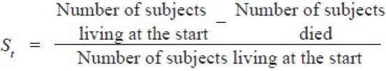
For each time interval, survival probability is calculated as the number of subjects surviving divided by the number of patients at risk. Subjects who have died, dropped out, or move out are not counted as “at risk” i.e., subjects who are lost are considered “censored” and are not counted in the denominator. Total probability of survival till that time interval is calculated by multiplying all the probabilities of survival at all time intervals preceding that time (by applying law of multiplication of probability to calculate cumulative probability). For example, the probability of a patient surviving two days after a kidney transplant can be considered to be probability of surviving the one day multiplied by the probability surviving the second day given that patient survived the first day. This second probability is called as a conditional probability. Although the probability calculated at any given interval is not very accurate because of the small number of events, the overall probability of surviving to each point is more accurate. Let us take a hypothetical data of a group of patients receiving standard anti-retroviral therapy. The data shows the time of survival (in days) among the patients entered in a clinical trial - (E.g. 1)- 6, 12, 21, 27, 32, 39, 43, 43, 46F^*, 89, 115F^*, 139F^*, 181F^*, 211F^*, 217F^*, 261, 263, 270, 295F^*, 311, 335F^*, 346F^*, 365F^* (^* means these patients are still surviving after mentioned days in the trial.)

We know about the time of the event, i.e. death in each subject, after he/she had entered the trial, may it be at different times. There are also a few subjects who are still surviving i.e. at the end of the trial. Even in these conditions we can calculate the Kaplan-Meier estimates as summarized in Table 1.

Table 1.

Kaplan-Meier estimate for patients mentioned in e.g. 1

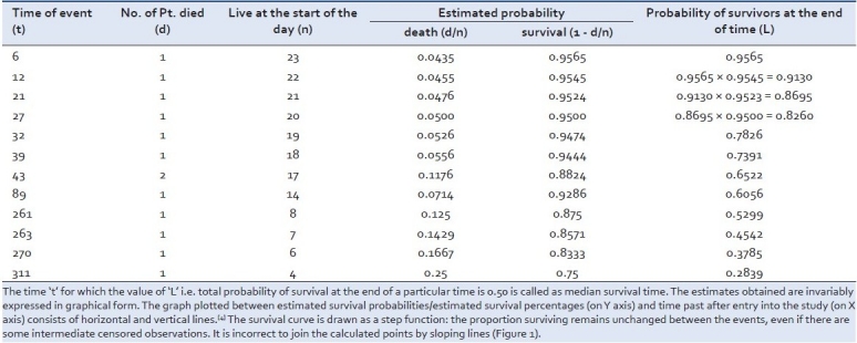
The time ‘t’ for which the value of ‘L’ i.e. total probability of survival at the end of a particular time is 0.50 is called as median survival time. The estimates obtained are invariably expressed in graphical form. The graph plotted between estimated survival probabilities/estimated survival percentages (on Y axis) and time past after entry into the study (on X axis) consists of horizontal and vertical lines.[4] The survival curve is drawn as a step function: the proportion surviving remains unchanged between the events, even if there are some intermediate censored observations. It is incorrect to join the calculated points by sloping lines [Figure 1].

Figure 1.

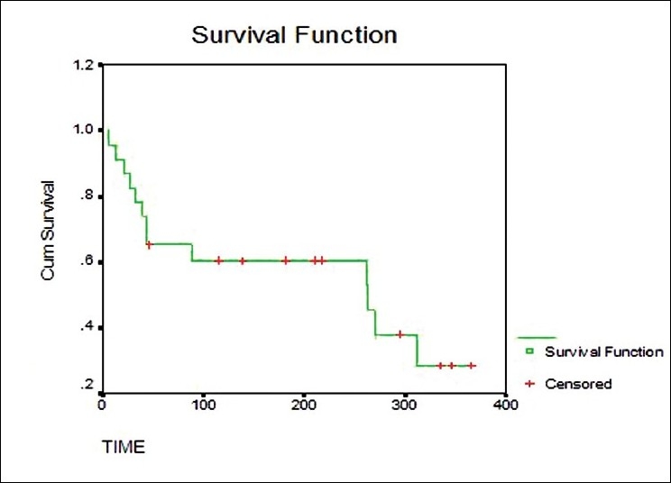
Plots of Kaplan-Meier product limit estimates of survival of a group of patients (as in e.g. 1) receiving ARV therapy

We can compare curves for two different groups of subjects. For example, compare the survival pattern for subjects on a standard therapy with a newer therapy. We can look for gaps in these curves in a horizontal or vertical direction. A vertical gap means that at a specific time point, one group had a greater fraction of subjects surviving. A horizontal gap means that it took longer for one group to experience a certain fraction of deaths.

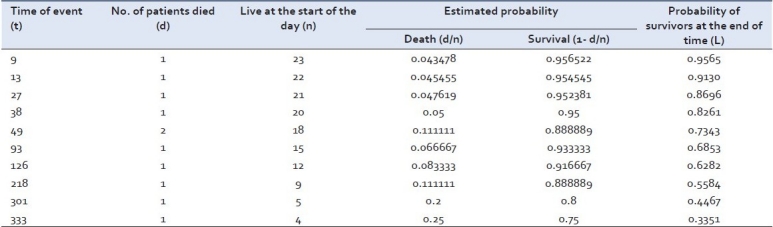
Let us take another hypothetical data for example of a group of patients receiving new Ayurvedic therapy for HIV infection. The data shows the time of survival (in days) among the patients entered in a clinical trial (as in e.g. 1) 9, 13, 27, 38, 45F^*, 49, 49, 79F^*, 93, 118F^*, 118F^*, 126, 159F^*, 211F^*, 218, 229F^*, 263F^*, 298F^*, 301, 333, 346F^*, 353F^*, 362F^* (^* means these patients are still surviving after mentioned days in the trial.)

The Kaplan-Meier estimate for the above example is summarized in Table 2.

Table 2.

Kaplan-Meier estimate (KM) for patients mentioned in e.g. 2

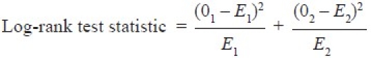
The two survival curves can be compared statistically by testing the null hypothesis i.e. there is no difference regarding survival among two interventions. This null hypothesis is statistically tested by another test known as log-rank test and Cox proportion hazard test.[5] In log-rank test we calculate the expected number of events in each group i.e. E₁ and E₂ while O₁ and O₂ are the total number of observed events in each group, respectively [Figure 2]. The test statistic is

Figure 2.

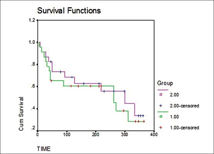
Plots of Kaplan-Meier product limit estimates of survival of a group of patients (as in e.g. 1 and 2) receiving ART and new Ayurvedic therapy for HIV Infection.

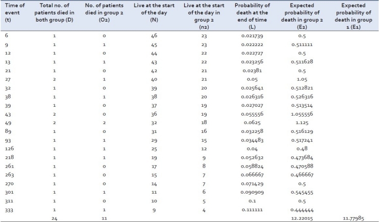
The total number of expected events in a group (e.g. E₂) is the sum of expected number of events, at the time of each event in any of the group, taking both groups together. At the time of event in any group the expected number of events is the product of risk of event at that time with the total number of subjects alive at the start of the time of event in that very group (e.g. at day 6, 46 patients were alive at the start of the day and one died, so the risk of event was 1/46 = 0.021739. As 23 patients were alive at the start of the day in group 2, the expected number of events at day 6 in group 2 was 23 × 0.021739 = 0.5). The total number of expected events in group 2 is sum of the expected events calculated at different time. The total number of expected events in the other group (i.e. E₁) is calculated by subtracting the total number of expected events in group 2 i.e. E ₂, from the total of observed events in both the groups i.e. O₁ + O₂.

Considering the above example the log-rank test can be applied as shown in Table 3.

Table 3.

Log-rank statistic for patients mentioned in examples 1 and 2

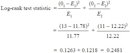
Computations of all the values in the above-mentioned formula will give test statistic value. The test statistic and the significance can be drawn by comparing the calculated value with the critical value (using chi-square table) for degree of freedom equal to one. The test statistic value is less than the critical value (using chi-square table) for degree of freedom equal to one. Hence, we can say that there is no significant difference between the two groups regarding the survival.

The log-rank test is used to test whether the difference between survival times between two groups is statistically different or not, but do not allow to test the effect of the other independent variables. Cox proportion hazard model enables us to test the effect of other independent variables on survival times of different groups of patients, just like the multiple regression model. Hazard is nothing but the dependent variable and can be defined as probability of dying at a given time assuming that the patients have survived up to that given time. Hazard ratio is also an important term and defined as the ratio of the risk of hazard occurring at any given time in one group compared with another group at that very time i.e. if H1, H2, H3 … and h1, h2, h3 … are the hazards at a given times T1, T2, T3… in group A and B, respectively, then hazard ratio at times T1, T2, T3 are H1/h1, H2/h2, H3/h3…, respectively. Both log-rank test and Cox proportion hazard test assume that the hazard ratio is constant over time i.e. in the above-mentioned scenario H1/h1 = H2/h2 = H3/h3.

To conclude, Kaplan-Meier method is a clever method of statistical treatment of survival times which not only makes proper allowances for those observations that are censored, but also makes use of the information from these subjects up to the time when they are censored. Such situations are common in Ayurveda research when two interventions are used and outcome assessed as survival of patients. So Kaplan-Meier method is a useful method that may play a significant role in generating evidence-based information on survival time.

REFERENCES

- 1.Armitage P, Berry G, Matthews JN. 4th ed. Oxford (UK): Blackwell Science; 2002. Clinical trials.Statistical methods in medical research; p. 591. [Google Scholar]
- 2.Berwick V, Cheek L, Ball J. Statistics review 12: Survival analysis. Crit Care. 2004;8:389–94. doi: 10.1186/cc2955. [DOI] [PMC free article] [PubMed] [Google Scholar]
- 3.Altman DG. London (UK): Chapman and Hall; 1992. Analysis of Survival times.In:Practical statistics for Medical research; pp. 365–93. [Google Scholar]
- 4.Indrayan A, Surmukaddam SB. Measurement of Community Health and Survival analysis. In: Chow SC, editor. Medical Biostatistics. Vol. 7. New York (US): Marcel Dekker; 2001. pp. 232–42. [Google Scholar]
- 5.Marubini E, Valsecchi MG. Chichester (UK): John Wiley and Sons; Chichester (UK): John Wiley and Sons; 1995. Estimation of Survival Probabilities.Analysing survival data from clinical trials and observational studies; pp. 41–8. [Google Scholar]