A Differential Autoregressive Modeling Approach within a Point Process Framework for Non-stationary Heartbeat Intervals Analysis

Abstract

Modeling heartbeat variability remains a challenging signal-processing goal in the presence of highly non-stationary cardiovascular control dynamics. We propose a novel differential autoregressive modeling approach within a point process probability framework for analyzing R-R interval and blood pressure variations. We apply the proposed model to both synthetic and experimental heartbeat intervals observed in time-varying conditions. The model is found to be extremely effective in tracking non-stationary heartbeat dynamics, as evidenced by the excellent goodness-of-fit performance. Results further demonstrate the ability of the method to appropriately quantify the non-stationary evolution of baroreflex sensitivity in changing physiological and pharmacological conditions.

I. Introduction

Recently, point process probability models have been advocated for characterizing human heartbeat intervals [1, 2, 3, 4, 5]. Unlike previous methods, the point process paradigm allows to estimate instantaneous heart rate (HR) and HR variability (HRV), as well as specific cardiovascular/cardiorespiratory functions such as respiratory sinus arrhythymia (RSA) or baroreflex sensitivity (BRS). In order to track the non-stationary heartbeat dynamics, an adaptive point process filtering approach has been proposed to trail the instantaneous model parameters [2, 4]. In this work, we propose a distinctive modeling perspective to tackle the non-stationary nature of the heartbeat intervals as well as potential other physiological covariates (such as blood pressure or respiration measures). The main feature of the proposed algorithm is the inclusion of a linear regression on the mean of the point process probability density by use of an autoregressive integrated moving average (ARIMA) model. Such framework also allows for a newly defined differential BRS index. Notably, the new index is conceptually similar to the time-domain “sequence method” [6, 9, 10], which has been often used to measure the sensitivity of the change of blood pressure (BP) relative to the change of R-R interval. However, more suitably in the presence of dynamic changes in a non-stationary environment, our index provides an instantaneous BRS characterization at arbitrarily small time resolutions.

The paper is organized as follows. We first present an overview of the point process modeling paradigm, the new frequency analysis framework associated with the ARIMA model, and the definition of the BRS index. We then apply the proposed model to both synthetic heartbeat series and experimental data recordings consisting of non-stationary heartbeat intervals and systolic BP during a propofol induction of anesthesia protocol [11] and a tilt-table protocol [1]. We demonstrate the noticeable improvement in model goodness-of-fit while fitting highly non-stationary recordings. Additionally, we use these examples to illustrate the ability of our new model to estimate the instantaneous differential BRS index. Finally, we conclude the paper with some discussions.

II. A Probability Model for Heartbeat Intervals

Given a set of R-wave events {u_j}_j=1^J detected from the electrocardiogram (ECG), let RR_j = u_j−u_j−1 > 0 denote the jth R-R interval. By treating the R-waves as discrete events, we develop a point process model for the heartbeat interval. Assuming history beat dependence, the waiting time t −u_j (t > u_j) until the next R-wave event can be modeled by an inverse Gaussian model [1]:

$$p(t)={\left(\frac{\theta }{2\pi t^3}\right)}^{\frac{1}{2}}\text{ exp }\left(-\frac{\theta {(t-u_j-{\mu }_{\text{RR}}(t))}^2}{2(t-u_j){\mu }_{\text{RR}}^2(t)}\right),$$

where u_j denotes the previous R-wave event occurred before time t, θ > 0 denotes the shape parameter, and μ_RR(t) denotes the instantaneous R-R mean. It is worth pointing out that when the mean μ_RR(t) is much greater than the variance, the inverse Gaussian can be well approximated by a Gaussian model with a variance σ_RR²(t) = μ_RR³(t)/θ:

$$p(t)={\left(\frac{1}{2\pi {\sigma }_{\text{RR}}^2(t)}\right)}^{\frac{1}{2}}\text{ exp }\left(-\frac{{(t-u_j-{\mu }_{\text{RR}}(t))}^2}{2{\sigma }_{\text{RR}}^2(t)}\right),$$

In point process theory, the inter-event probability p(t) is related to the conditional intensity function (CIF) λ(t) by a one-to-one transformation: $\lambda (t)=\frac{p(t)}{1-{\displaystyle {\int }_{u_j}^{t}p(\tau )\mathrm{d}\tau }}$. The estimated CIF can be used to evaluate the goodness-of-fit of the point process model for the heartbeat intervals.

A. Instantaneous Indices of HR and HRV

Heart rate (HR) is defined as the reciprocal of the R-R intervals. For time t measured in seconds, the new variable r = c(t −u_j)⁻¹ (where c = 60 s/min) can be defined in beats per minute (bpm). By the change-of-variables formula, the HR probability p(r) = p(c(t −u_j)⁻¹) is given by $p(r)=|\frac{\mathrm{d}t}{\mathrm{d}r}|p(t)$, and the mean and the standard deviation of HR r can be derived [1]:

$${\mu }_{\text{HR}}={\tilde{\mu }}^{-1}+{\tilde{\theta }}^{-1},{\sigma }_{\text{HR}}=\sqrt{(2\tilde{\mu }+\tilde{\theta })/\tilde{\mu }{\tilde{\theta }}^2},$$ (1)

where μ̃ = c⁻¹ μ_RR and θ̃ = c⁻¹ θ. Essentially, the instantaneous indices of HR and HRV are characterized by the mean μ_HR and standard deviation σ_HR, respectively.

B. Modeling of Instantaneous Heartbeat Interval’s Mean

In general, the heartbeat interval can be modeled by Wiener-Volterra series expansion, using previous R-R intervals and other physiological covariates (e.g., blood pressure or respiration) as the input variables. Although inclusion of nonlinear or bilinear terms in modeling is possible [3, 5], in this paper we focus on the investigation on linear modeling approaches.

1) AR Modeling

We can use the bivariate AR model to model the instantaneous mean μ_RR(t) [3]:

$${\mu }_{\text{RR}}(t)=a_0(t)+{\displaystyle \sum _{i=1}^p{a}_i(t){\mathit{\text{RR}}}_{t-i}+}{\displaystyle \sum _{j=1}^p{b}_j(t){\mathit{\text{BP}}}_{t-j}}$$ (2)

where a₀ compensates the nonzero mean effect of the R-R measurements, {RR_t−i}_i=1^p represents previous p R-R series prior to time t, and BP_t−j denotes the previous jth systolic blood pressure (BP) value prior to time t. The BP in (2) can be represented by the systolic beat-to-beat BP values. Note that the AR coefficients {a_i(t)} and {b_j(t)} in the above equation are time-varying, thus allowing to account for non-stationarity. However, when the R-R series and/or BP series contain non-stationary dynamics not directly associated with the cardiovascular control elicited oscillations (for example a linear increasing or decreasing trend), the AR coefficients have to be updated to account for such trends, and their evolution may track less effectively the non-stationarities of real interest.

2) ARIMA Modeling

In time-series (linear) modeling, it is a common practice to “detrend” a time series by taking differences if the series exhibits undesired non-stationary features. The autoregressive integrated moving average (ARIMA) process may provide a suitable framework to achieve such goal from a modeling point of view [12]. Simply, the original time series is applied by a difference operator (one or more times) until the non-stationary trends are not observed in the final series of interest. Motivated by this idea, we here define the “increment of R-R series” {δRR_t−i}≡{RR_t−i−RR_t−i−1} and the “increment of SBP series” {δBP_t−j}≡{BP_t−j−BP_t−j−1}, and model the instantaneous heartbeat interval mean by the following new equation:

$${\mu }_{\text{RR}}(t)={\mathit{\text{RR}}}_{t-1}+{\displaystyle \sum _{i=1}^p{a}_i(t)\delta {\mathit{\text{RR}}}_{t-i}+}{\displaystyle \sum _{j=1}^p{b}_j(t)\delta {\mathit{\text{BP}}}_{t-j}}.$$ (3)

Note that the a₀(t) term in (2) has been replaced by RR_t−1 in (3).

C. Adaptive Point Process Filtering

Let ξ = [{a_i}_i=1^p,{b_j}_j=1^p,θ]^T denote the vector that contains all unknown parameters from the new model (3), we can recursively estimate them via adaptive point process filtering [2]:

$$\begin{array}{cc}\hfill & {\xi }_{k|k-1}={\xi }_{k-1|k-1}\hfill \\ \hfill & P_{k|k-1}=P_{k-1|k-1}+W\hfill \\ \hfill & {\xi }_{k|k}={\xi }_{k|k-1}+P_{k|k-1}(\nabla \text{log}{\lambda }_k)[n_k-{\lambda }_k\mathrm{\Delta }]\hfill \\ P_{k|k}=\hfill & {\left[P_{k|k-1}^{-1}+\nabla {\lambda }_k\nabla {\lambda }_k^T\frac{\mathrm{\Delta }}{{\lambda }_k}-{\nabla }^2\text{log}{\lambda }_k[n_k-{\lambda }_k\mathrm{\Delta }]\right]}^{-1}\hfill \end{array}$$

where P and W denote the parameter and noise covariance matrices, respectively; and Δ=5 ms denotes the time bin size. Symbols $\nabla {\lambda }_k=\frac{\partial {\lambda }_k}{\partial {\xi }_k}\text{ and }{\nabla }^2{\lambda }_k=\frac{{\partial }^2{\lambda }_k}{\partial {\xi }_k\partial {\xi }_k^T}$ denote the first- and second-order partial derivatives of the CIF w.r.t. ξ at time t = kΔ, respectively. The indicator variable n_k = 1 if a heart beat occurs in time ((k−1)Δ, kΔ] and 0 otherwise.

D. Goodness-of-fit Tests

The goodness-of-fit of the point process model is tested based on the time-rescaling theorem [1, 2]. Given a point process specified by J discrete events: 0 < u₁ < …< u_J < T, define the random variables $z_j={\displaystyle {\int }_{u_{j-1}}^{u_j}\lambda (\tau )d\tau \text{ for }\mathit{j}=\mathit{1},\mathit{2},\mathbf{\dots },\mathit{J}-\mathit{1}}$ . Then the random variables z_js are independent, unit-mean exponentially distributed. By introducing the variable of transformation v_j = 1−exp(−z_j), then the v_js are independent, uniformly distributed within the region [0, 1]. Let g_j = Φ⁻¹(v_j) (where Φ(·) denotes the cumulative density function (cdf) of the standard Gaussian distribution), then the g_js will be independent standard Gaussian random variables. The Kolmogorov-Smirnov (KS) test is used to compare the cdf of the v_j against that of the random variables uniformly distributed in [0, 1]. The KS statistic meausres the maximum deviation of the empirical cdf from the uniform cdf. To visualize the KS plot, the v_js are sorted from the smallest to the largest value, then we plot values of the cdf of the uniform density defined as $\frac{j-0.5}{J}$ against the ordered v_js, and the 95% confidence interval lines are defined by $\mathit{y}=\mathit{x}\pm \frac{1.36}{{(J-1)}^{1/2}}$. When the model matches the data, the KS plot shall fall within the 95% confidence bounds.

In addition, the autocorrelation function of the g_js, defined by $\mathit{\text{ACF}}(m)=\frac{1}{J-m}{\displaystyle {\sum }_{j=1}^{J-m}{g}_j{g}_{j+m}}$ , is computed. If the g_js are independent, they are also uncorrelated; hence, ACF(m) shall be small (around 0 and within the 95% confidence interval $\frac{1.96}{{(J-1)}^{1/2}}$) for all values of m.

III. Frequency Analysis for Differential BRS

In light of equation (3), we can derive the instantaneous BP→RR transfer function in the feedback loop, which essentially relates to the differential BRS

$$H(f,t)=\frac{{\displaystyle {\sum }_{i=1}^q{b}_i(t)z^{-i}{|}_{z=e^{j2\pi f_2}}}}{1-{\displaystyle {\sum }_{i=1}^p{a}_i(t)z^{-i}{|}_{z=e^{j2\pi f_1}}}}.$$ (4)

Note that the new form of transfer function is reminiscent of the “sequence method” [6, 9, 10] previously used to define the BRS. However, the sequence method employed a time-domain batch method, while ours is a frequency-domain instantaneous method. We further assume that the effect of time discretization is small such that the linear dependence between two variables remains unchanged, i.e. $\frac{y(t)}{x(t)}\mathbf{\approx }\frac{y(t+\delta )-y(t)}{x(t+\delta )-x(t)}$. As expected, due to the difference operator used in the time domain, the new AR coefficients {a_i,b_i} are more sensitive to the “incremental changes”; consequently, in the frequency domain, |H(f,t)| would amplify the baroreflex gain assessment (especially in the high-frequency range).

IV. Data and Results

A. Simulation

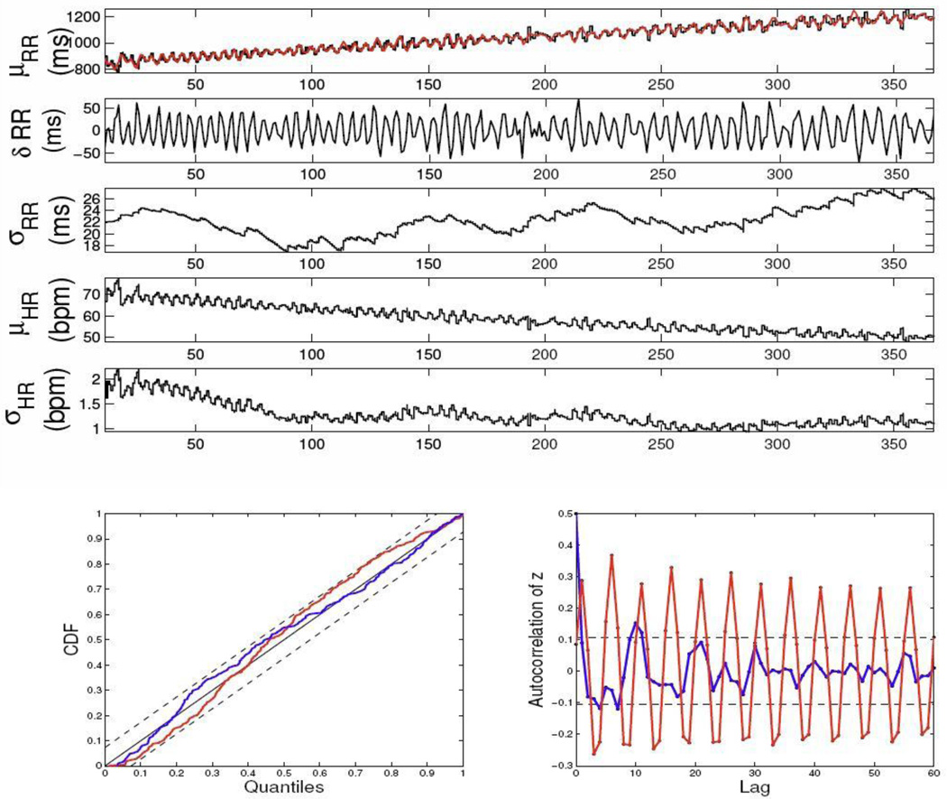
We simulated the heartbeat R-R series (unit: ms) using a stationary linear Gaussian model plus a linear increasing trend along time (for simplicity, we use only a univariate AR model in simulation):

$$({\mathit{\text{RR}}}_{t-1}-1000)=\alpha t+{\displaystyle \sum _{i=1}^8{a}_i({\mathit{\text{RR}}}_{t-i}-1000)+n(t)}$$ (5)

where α=0.001, and n(t) is a Gaussian noise process with zero mean and variance of 100. As seen from the top panel of Fig. 1, the simulated R-R series has a linear increasing trend (from ~800 ms to ~1200 ms) during a 6-min interval. The overall R-R series has a global mean of 1000 ms and standard deviance of 110. The AR coefficients {a_i} used to generate the series were previously estimated from stationary experimental recordings. The estimated instantaneous HR and HRV indices are shown in Fig. 1. The assessment of goodness-of-fit for the new differential AR formulation (4) indicates that the model provides an excellent characterization of the non-stationary R-R interval series (Fig. 1). Furthermore, the differential regression model achieves a better KS statistic (0.059) than a model with standard linear regression (0.072), although both models fall within the 95% confidence intervals. Of note, the autocorrelation plot is also significantly improved by using the differential regression, probably because the AR structure in the standard regression would require a higher regressive order to capture the non-stationary nature of the beat intervals—this can be confirmed by the oscillatory shape in the autocorrelation plot. Overall, this example illustrates how the model perspective (i.e., the ARIMA modeling) and the algorithm perspective (i.e., point process adaptive filtering) are equally important for tracking non-stationarities. An inappropriately chosen model (even empowered by adaptive point process filtering) would inevitably lead to unsatisfactory characterization of particular non-stationary dynamics in the heartbeat interval data.

Figure 1.

Simulated R-R interval series (top panel, red trace) and the estimated instantaneous indices, as well as the KS plots and autocorrelation plots obtained from two models (Eqs. 3 and 4) for the instantaneous R-R mean. The KS statistic is improved from 0.072 (old model, red curve) to 0.059 (new model, blue curve).

B. Experimental Data: Induction of General Anesthesia

We analyzed the experimental recordings from a general anesthesia experiment. The experimental protocol was approved by the Massachusetts General Hospital (MGH) Department of Anesthesia and Critical Clinical Practices Committee, the MGH Human Research Committee and the MGH General Clinical Research Center, and has been reported previously [3, 11]. Briefly, subjects were delivered several concentration levels of propofol anesthetic drug (0.0, 1.0, …, 5.0 µg/ml) administered by anesthesiologists. Each epoch lasted about 15 minutes.

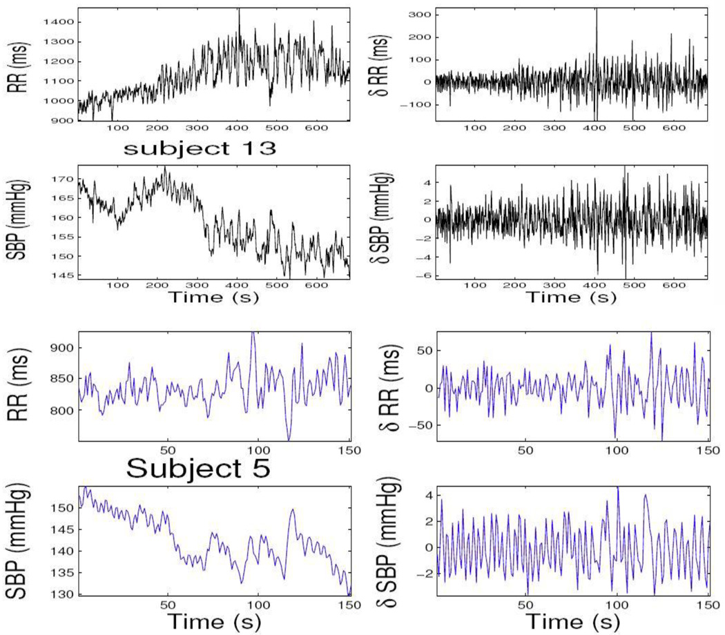
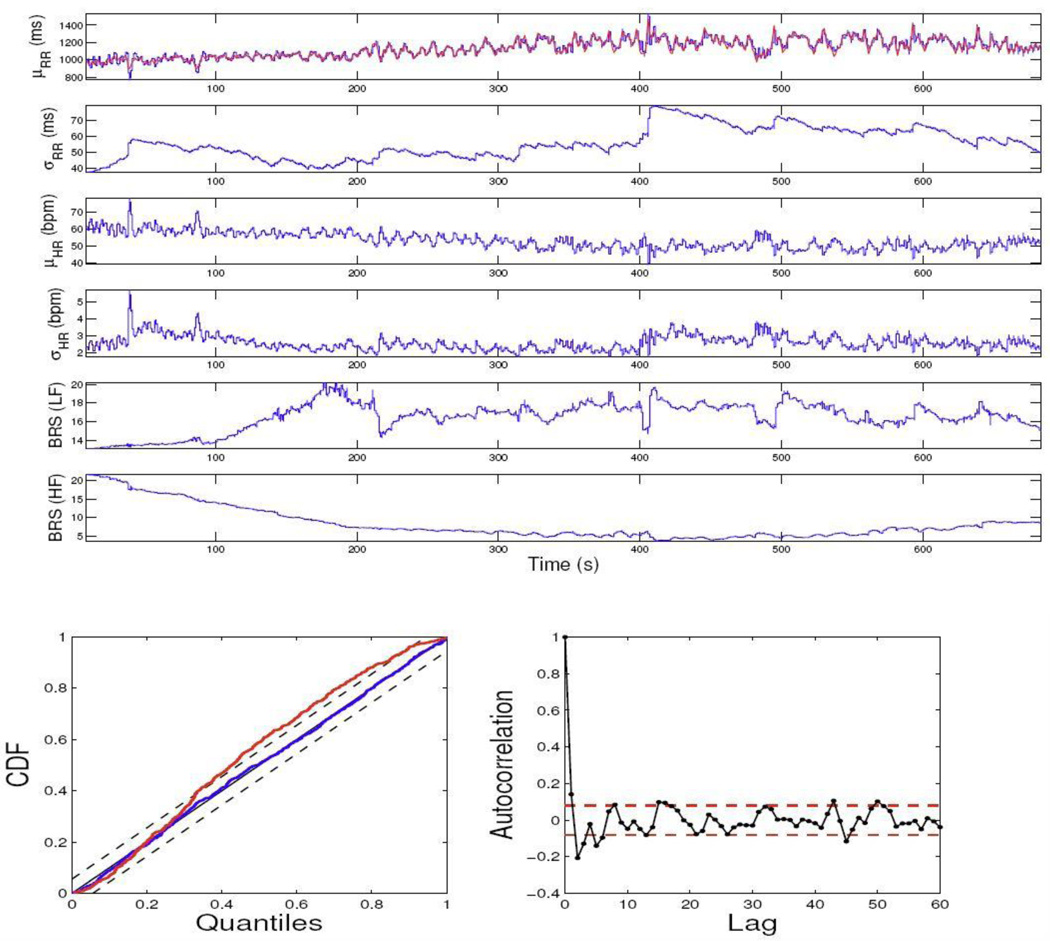
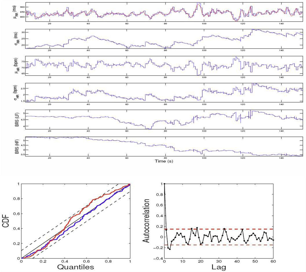
In examining the data, we have observed that upon propofol administration, the physiological measurements exhibit highly non-stationary dynamics (as opposed to the awake baseline steady state), which brings in the challenge of correctly modeling these data while simultaneously assessing cardiovascular control. Here, we consider only two experimental epochs during induction of anesthesia (level-1 propofol concentration) to illustrate our model. The experimental data recordings from two subjects are shown in Fig. 2. The model parameters in (3) are initialized by fitting a bivariate AR model with a least-squares method on the first 100 samples. The model order p is chosen from 4 to 8 and the final optimum order is chosen according to the Akaike information criterion (AIC). The estimated instantaneous HR, HRV, and BRS indices from two subjects are shown in Figs. 3 and 4, along with the KS plot and autocorrelation plot. As seen, the KS plots are almost aligned with 45° line, indicating a nearly perfect model fit.

Figure 2.

Two experimental R-R interval series and SBP series (left panels) from two recording epochs during level-1 propofol concentration. Their corresponding incremental series are also shown at the right panels. In subject 13, R-R series has a clear increasing trend. In both subject 13 and subject 5, the SBP series has a clear decreasing trend.

Figure 3.

The estimated instantaneous indices from the data of subject 13 and the associated KS and autocorrelation plots. The KS statistic is improved from 0.0681 (old model, red curve) to 0.0152 (new model, blue curve).

Figure 4.

The estimated instantaneous indices from the data of subject 5 and the associated KS and autocorrelation plots. The KS statistic is improved from 0.0893 (old model, red curve) to 0.0513 (new model, blue curve).

C. Experimental Data: Tilt-Table

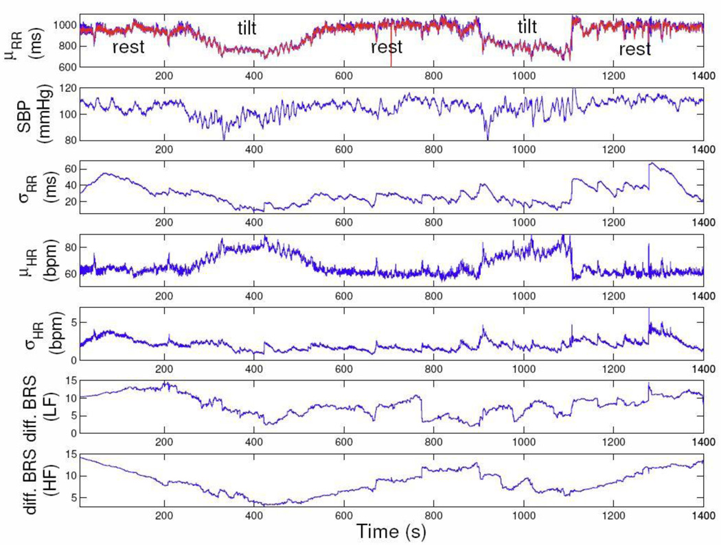
Finally, we considered R-R intervals and SBP recordings, from a protocol where each subject underwent a few cycles of “rest” and “tilt” posture conditions (details of the “tilt-table” protocol can be found in [1]). For demonstration purpose, we analyzed two representative subjects (#1 and #4). As an illustration, Figure 5 shows the estimated instantaneous indices from Subject #1 (only 5 cycles are shown). As seen, the point process filter tracks the instantaneous differential BRS with fluctuating trend similar to R-R intervals, i.e. decreasing during tilt and increasing back to baseline level as the subject returned to supine position. For statistical analysis, we averaged the differential BRS estimates (HF range) along the “rest” and “tilt” epochs (values are shown in Table I). Notably, comparing the tilt epochs with the rest epochs, the mean differential BRS is lower, in agreement with consolidated previous findings in the literature [7, 8]. As further comparison, we also computed the BRS using the sequence methods (one value for each epoch, as the sequence method cannot perform an instantaneous assessment). The slope of the linear interrelation between SBP and the next R-R interval is calculated when the correlation coefficient is at least 0.7 (violation of this condition will inevitably make the slope estimate inaccurate). As seen from the table, the significant decrease in differential BRS from rest to tilt are confirmed by both methods, with the point process measure providing a more accurate representation in terms of both timescale and methodology.

Figure 5.

The estimated instantaneous indices from one subject from the tilt-table data set.

Table 1.

Comparison of the differential BRS estimate in the “rest” and “tilt” epochs. The mean and SD statistics are computed by averaging all epochs for each subject.

	our method (HF)		sequence method
	Subject #1	Subject #4	Subject #1	Subject #4
rest	8.54 ± 2.88	5.36 ± 1.35	15.87 ± 6.36	7.82 ± 2.07
tilt	5.76 ± 2.06	4.65 ± 0.99	3.70 ± 0.51	3.28 ± 0.86

V. Summary and Discussion

We propose a novel differential autoregressive modeling approach within a point process probability framework for analyzing R-R interval and blood pressure variations. In testing the proposed model as applied to synthetic and experimental data in highly non-stationary conditions, the model is found to be greatly effective in tracking non-stationary heartbeat dynamics, as evidenced by excellent goodness-of-fit performance. In addition to producing optimal KS statistics, the new model also includes the computational advantage of allowing for lower autoregressive orders, as the incremental series exhibit more stationary features. The differential BRS assessment proves as a valid instantaneous characterization at arbitrarily small time resolutions Overall, the new formulation allows for more precise dynamic measures in a highly non-stationary environment, and provides one further advancement towards potential realtime indicators for ambulatory monitoring and instantaneous assessment of autonomic control in clinical practice.

References

- 1.Barbieri R, Matten EC, Alabi AA, Brown EN. A point-process model of human heartbeat intervals: new definitions of heart rate and heart rate variability. Am J. Physiol. Heart Cicr. Physiol. 2005;vol. 288:424–435. doi: 10.1152/ajpheart.00482.2003. [DOI] [PubMed] [Google Scholar]
- 2.Barbieri R, Brown EN. Analysis of heart beat dynamics by point process adaptive filtering. IEEE Trans. Biomed. Eng. 2006;vol. 53(no. 1):4–12. doi: 10.1109/tbme.2005.859779. [DOI] [PubMed] [Google Scholar]
- 3.Chen Z, Purdon PL, Pierce ET, Harrell G, Brown EN, Barbieri R. Assessment of baroreflex control of heart rate during general anesthesia using a point process method; Proc. ICASSP’09; Taiwan: 2009. pp. 333–336. [DOI] [PMC free article] [PubMed] [Google Scholar]
- 4.Chen Z, Brown EN, Barbieri R. Assessment of autonomic control and respiratory sinus arrhythmia using point process models of human heart beat dynamics. IEEE Trans. Biomed. Eng. 2009;vol. 56:1791–1802. doi: 10.1109/TBME.2009.2016349. [DOI] [PMC free article] [PubMed] [Google Scholar]
- 5.Chen Z, Brown EN, Barbieri R. Characterizing nonlinear heartbeat dynamics within a point process framework. IEEE Trans. Biomed. Eng. 2010;vol. 57(no. 6):1335–1347. doi: 10.1109/TBME.2010.2041002. [DOI] [PMC free article] [PubMed] [Google Scholar]
- 6.Hughson RL, Quintin L, Annat G, Yamamoto Y, Gharib C. Spontaneous baroreflex by sequence and power spectral methods in humans. Clin. Physiol. 1993;vol. 13(no. 6):663–676. doi: 10.1111/j.1475-097x.1993.tb00481.x. [DOI] [PubMed] [Google Scholar]
- 7.Malliani A, Pagani M, Lombardi F, Cerutti S. Cardiovascular neural regulation explored in the frequency domain. Circulation. 1991;vol. 84:1482–1492. doi: 10.1161/01.cir.84.2.482. [DOI] [PubMed] [Google Scholar]
- 8.Montano N, Ruscone T, Porta A, et al. Power spectrum analysis of heart rate variability to as- sess the changes in sympathovagal balance during graded orthostatic tilt. Circulation. 1994;vol. 90:1826–1831. doi: 10.1161/01.cir.90.4.1826. [DOI] [PubMed] [Google Scholar]
- 9.Oka H, Mochio S, Yoshioka M, Morita M, Inoue K. Evaluation of baroreflex sensitivity by the sequence method using blood pressure oscillations and R-R interval changes during deep respiration. Eur. Neurol. 2003;vol. 50:230–243. doi: 10.1159/000073865. [DOI] [PubMed] [Google Scholar]
- 10.Parati G, DiRienzo M, Mancia G. Dynamic modulation of baroreflex sensitivity in health and disease. Ann. NY Acad. Sci. 2001;vol. 940:469–487. doi: 10.1111/j.1749-6632.2001.tb03699.x. [DOI] [PubMed] [Google Scholar]
- 11.Purdon PL, et al. Simultaneous electroencephalography and functional magnetic resonance imaging of general anesthesia. Ann. NY Acad. Sci. 2009;vol. 1157:61–70. doi: 10.1111/j.1749-6632.2008.04119.x. [DOI] [PMC free article] [PubMed] [Google Scholar]
- 12.Vu KM. The ARIMA and VARIMA Time Series: Their Modelings, Analyses and Applications. 2007 [Google Scholar]