EPIBLASTER-fast exhaustive two-locus epistasis detection strategy using graphical processing units

Abstract

Detection of epistatic interaction between loci has been postulated to provide a more in-depth understanding of the complex biological and biochemical pathways underlying human diseases. Studying the interaction between two loci is the natural progression following traditional and well-established single locus analysis. However, the added costs and time duration required for the computation involved have thus far deterred researchers from pursuing a genome-wide analysis of epistasis. In this paper, we propose a method allowing such analysis to be conducted very rapidly. The method, dubbed EPIBLASTER, is applicable to case–control studies and consists of a two-step process in which the difference in Pearson's correlation coefficients is computed between controls and cases across all possible SNP pairs as an indication of significant interaction warranting further analysis. For the subset of interactions deemed potentially significant, a second-stage analysis is performed using the likelihood ratio test from the logistic regression to obtain the P-value for the estimated coefficients of the individual effects and the interaction term. The algorithm is implemented using the parallel computational capability of commercially available graphical processing units to greatly reduce the computation time involved. In the current setup and example data sets (211 cases, 222 controls, 299468 SNPs; and 601 cases, 825 controls, 291095 SNPs), this coefficient evaluation stage can be completed in roughly 1 day. Our method allows for exhaustive and rapid detection of significant SNP pair interactions without imposing significant marginal effects of the single loci involved in the pair.

Introduction

Understanding the effects of genes on phenotypes and diseases has long been suggested to embed a complex form of interaction as a result of inter-inhibitory and -excitatory effects, with any attempt to explain these effects simply as additive effects of the individual genes being an overly simplistic model that ultimately provides an incorrect view of the genetic influence on the phenotype.

The study of interactions between polymorphic loci can stem from both a biological and statistical genetics perspective. The first approach establishes a model based on a priori knowledge of how the genes function and interact. The latter, being a ‘biological blind' approach, helps to draw inferences from previously unknown interdependencies between genes. The ultimate objective, similar to all black-box studies, is to merge the conclusions drawn from both approaches; however, as the observations made cannot be measured at a level more finite than the eventual system output, the former approach is more likely to be refined by first having a solid statistical finding as its basis.

As our effort primarily focuses on drawing statistical inference on epistatic actions/interactions between genes, a new method is proposed to help improve our capability to search and sift out significant interactions. This paper will discuss the performance of our method in its current implementation. The results applied to a simulated subset of SNPs and to two real genome-wide data sets recorded from panic disorder and multiple sclerosis studies will be presented, followed by a discussion of some properties of the approach.

Materials and methods

Overview of the two-stage search strategy

The strategy consists of a two-stage approach. First, a filtering stage using the difference of Pearson's correlation coefficients that performs an exhaustive two-locus interaction multiplicative effects¹ search across all possible pairwise SNP combinations is performed. This is followed by logistic regression analysis on those subset of pairs deemed significant in the previous stage.

Data representation

Each SNP is represented as integer values ranging from 0 to 2 based on the count of a chosen reference nucleotide of the selected SNP for an allele dosage model, or as 0 or 1 depending on the genotype for a dominance or recessivity coding. In the current study, the allele dosage model is applied. An overall matrix is generated to store the information of all SNPs as column vectors and the recorded values for individual subjects along the rows. Column vectors are then analyzed in pairs and the correlation coefficients are tabulated for cases and controls separately. Correlation coefficients are calculated from a 3 × 3 ordered genotype matrix, the genotypes being encoded 0, 1, 2. The difference between the correlation coefficients in cases and controls is then computed and used as an indication of the SNP pair contributing significantly to the classification between cases and controls (equation (1)).

Correlation coefficients (Pearson's) difference between case-only and control-only for each SNP–SNP pair. Note that no assumptions, such as HWE to hold, are needed here.

Difference of correlation coefficients=Δ

The variance of each of these correlation coefficients is, as shown by Wellek and Ziegler,² equal to 1/(n−1), where n is the respective number of cases and controls. As the cases and controls obviously constitute, independent samples, the total variance V_tot is then the sum of the two single variances. As a consequence, and from both Gretton et al³ and Wellek and Ziegler,² we can conclude that T=ΔV_tot^1/2 ∼ N(0, 1).

The first stage of analyzing the difference of correlations approach searches for significant interaction terms. The second stage then computes the fit using a full rank logistic model (equation (2)), including the intercept and additive marginal effects, on the subset of loci pairing deemed significant from the first stage, from which a statistical test can be conducted to test for the coefficient of interaction term being significantly different from zero.

Full rank logistic regression model:

Hardware and software setup

The hardware used in the experimental setup consists of two pairs of commercially available NVIDIA GTX295 GPUs (Santa Clara, CA, USA) running on an Intel Core i7 920 with 2.67 GHz (Santa Clara, CA, USA) central processing unit host (CPU) using 12 GB of DDR3 RAM (Corsair Inc., Fremont, CA, USA). The software program is implemented in R (version 2.9.2; R Development Core Team⁴) with the ‘gputools' package beta version 0.1-4 (Buckner et al⁵) installed (http://cran.r-project.org/web/packages/gputools), in which the function ‘gpuCor' permits correlation coefficients to be tabulated for all possible pairwise interactions across the column vectors using the Compute Unified Device Architecture (CUDA)-enabled NVIDIA graphic cards. The graphical card uses its parallel computational capability to process independent evaluations faster than conventional CPU-based computation. As the correlation coefficients between each SNP pair can be tabulated independently, this can take full advantage of the inherent parallel computation performed on graphical cards. The overall time performance depends on the sample size and desired marker coverage. A total evaluation of (number of SNPs choose 2) interactions is typically accomplished within 24 h for the entire data set (2000 individuals consisting of 1000 cases, 1000 controls with 500 000 SNPs) with the available GPU resources and the given results retention criteria. Limitations on speed can originate from local main memory storage, memory transfer speed and number of on-board GPU cores present. Some data partitioning to take advantage of all current GPU resource are thus required to render this method most efficient. The data set for the study is first partitioned into blocks containing 2000 SNPs each, which can be handled by the memory on the graphic card. Hence, for a genome-wide data set of 500K SNPs, 250 partitions are required.

The process goes through the entire data set and calculates the correlation coefficients in blocks of 2000 SNPs. The very first correlation analysis performed is on the first partition to itself, a ‘partition-based autocorrelation', resulting in 1 999 000 unique correlations. The process then increases the partition index of the second partition by one and completes a correlation between two distinct sets of 2000 SNPs, a ‘partition-based cross-correlation', to yield 4 million unique results. This process of increasing the nested loop index is repeated until it reaches the last partition set, at which point the top-level loop index gets increased by one. The process can be summarized in the following steps:

1. Partition the data set into a size of 2000 SNPs. Note that this number may increase or decrease depending on the number of individuals studied.

2. Set up a two-level nested loop to apply the partition-based correlation for all possible SNP pairs for cases and controls separately.

3. Compute the difference of correlation coefficients between cases and controls after each partition-based autocorrelation or cross-correlation is complete.

4. Compute the P-values of each difference given that the distribution of the differences follows a Gaussian distribution (refer to the Results section).

5. Retain only SNP pairs that show a P-value below a selected threshold.

6. Repeat steps 3–5 across all partition pairs.

7. Proceed to stage 2 by performing a logistic regression on the selected pairs.

Results

Simulated data

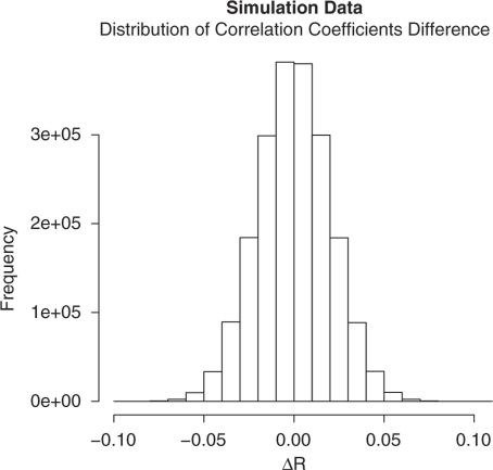
A simulated data set is generated consisting of 2000 SNPs and a subject size of 5000 controls and 5000 cases. This simulated data set is created without any specific model allowing for any a priori knowledge of which particular pair will be significant. The purpose is to demonstrate validity in the approximation of the resulting logistic regression interaction term P-value to the approximation based on the difference in correlation coefficients. The distribution of the differences of correlation coefficients is noted to exhibit a Gaussian distribution within each partition set, referring to the histogram plot in Figure 1. This observation has been examined in greater detail by Gretton et al,³ stating that when samples are indeed drawn from two different distributions the distribution of the discrepancy of the chosen function, difference of estimated mean correlation coefficients in this study, will converge to a Gaussian distribution. An additional proof for the difference of correlation coefficients to exhibit a Gaussian distribution can be found in Wellek and Ziegler,² who have also shown that the variance of any single difference under the null hypothesis and thus also of the distribution of the sum of all differences is the sum of the reciprocals of the number of cases and controls. For this Gaussianism, equal numbers of cases and controls are not needed.

Figure 1.

Histogram of differences of correlation coefficients of all two-way interactions of 2000 SNPs exhibiting the expected Gaussian distribution shape.

In practice, to test for the significance of each pair, a Z-score is tabulated for each difference within the partition set. This Z-score is computed on the basis of the mean and standard deviation of all the differences noted within the partition set, which is a close approximation to the overall mean and standard deviation, given that the partition size is chosen to be large enough, typically resulting in a few million pairs for each partition set. Those interactions exhibiting a high overall Z-score are then taken as an indication that the effect of the interaction term of the two SNPs in question is deemed valuable enough to be passed on to the second stage. This filtered subset is then subjected to a second level of mathematical-intensive evaluation using the likelihood ratio test on the logistic regression model.

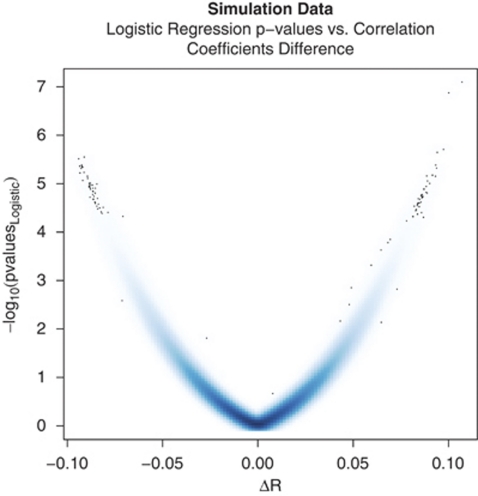
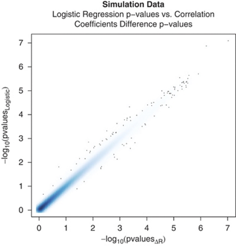
Referring to Figure 2, the P-values of the interaction product term in a general linear fit are plotted against their correlation coefficient differences between cases and controls. To help delineate any logarithmic trend, the P-values are shown as negative logarithmic values. As shown in Figure 2, there is a strong relationship between the two variables, of a parabolic function in the region centered around the origin to a linear relationship in the region of higher values. The region that is of most interest to the study is the higher numerical value region, as the P-values are the smallest and the differences are the largest. As the differences closely follow a Gaussian distribution (Figure 1), a Z-score threshold can be used to estimate the retention rate. The statistic is then estimated using the fact that the Z-score would follow a standard T-distribution with a sufficiently large number of degrees of freedom. A plot comparing the P-values obtained between the approximation and the validation step is illustrated in Figure 3 and demonstrates a high R² value of 99.9%.

Figure 2.

Logarithmic P-values from the interaction term of logistic regression versus correlation coefficient differences of all two-way interactions from 2000 SNPs.

Figure 3.

Logarithmic P-values from the interaction term of the logistic regression model versus correlation coefficient differences P-values from 2000 SNPs (2000C2=1999000 SNP–SNP pairs). Quality of fit (R²) between the P-values is 99.9%.

To help address the issues of limited physical disk space and of retaining only those interactions that show strong significance, a Z-score of 4.5 was chosen as the cutoff threshold, which corresponds to a probability of 6.8 × 10⁻⁶ retention rate. Thus, for the partition-based autocorrelation generating ∼2 million (2000 choose 2) correlation coefficient differences, only the top 14 interaction pairs are expected to be retained. Overall, we expect the top ∼8.5 × 10⁶ pairs out of a possible ∼1.25 × 10¹¹ retained from the first stage in a marker coverage of 500K SNPs.

Real data

Real genetic data have been recruited from two separate published studies. The first data set originated from a panic disorder study⁶ with a total of 299 468 SNPs, where 211 cases and 222 controls have been retained after standard quality control measures. Computing the difference of correlation coefficients across all pairs and choosing a P-value threshold of 1.0 × 10⁻⁵ resulted in a retention of 373 153 SNP pairs. Similarly, a second larger data set from a multiple sclerosis⁷ study with a total of 291 095 SNPs in 601 cases and 825 controls is also being investigated. Using the same P-value threshold of 1.0 × 10⁻⁵, the 407 660 most significant SNP pairs are retained upon subjecting it to the first stage.

In view of verifying that indeed no significant pairs have been left out in the adopted difference-of-correlation-coefficients stage of our method, a comparison to the P-values of the interaction term in a normal linear regression of all possible SNP pairs must be made. To perform this brute-force approach in a time efficient manner, we have used a newly released software tool, FastEpistasis (http://www.vital-it.ch/software/FastEpistasis),⁸ which is an extension of the PLINK epistasis module capable of distributing the work in parallel on multiple CPU cores. It is important to point out that this method is not working on the difference of odds ratio as conducted by the Plink option bearing the same name. The program is meant to be executed on quantitative phenotypes, but the difference in P-values, which are the relevant measure for this comparison, has been noted to be negligible on several sample SNP pairs (see also Table 1, comparing the FastEpistasis column with the logistic regression interaction term P-value column, and also simulation studies (Supplementary Figure 1)). The P-values computed from FastEpistasis is regarded to be the ‘true' value used for comparison with the approximated method described in stage 1 of EPIBLASTER.

Table 1. Top 10 panic disorder SNP pairs differences of correlation coefficient, FastEpistasis and logistic regression P-values.

Top 10 panic disorder SNP pairs ranked by FastEpistasis
Ranking	SNP1 Name	SNP2 Name	Difference of R	Difference of R P-value	FastEpistasis P-value	Lreg-SNP1 P-value	Lreg-SNP2 P-value	Lreg-interaction P-value
1	rs4653309	rs17338700	0.6111244	2.26E-10	6.97E-12	1.94E-01	6.16E-01	8.98E-12
2	rs4984422	rs1967113	−0.6582624	8.86E-12	1.06E-11	2.02E-01	8.66E-01	4.72E-13
3	rs1156847	rs7246846	0.620029	1.21E-10	6.57E-11	7.45E-01	2.01E-01	4.02E-11
4	rs6455842	rs265548	0.6423732	2.81E-11	7.25E-11	3.67E-01	3.55E-01	6.17E-12
5	rs12188192	rs1317584	0.5777778	1.98E-09	8.08E-11	2.51E-01	4.90E-01	1.87E-10
6	rs2100807	rs4875302	0.6104409	1.95E-10	1.88E-10	7.15E-01	3.95E-01	1.45E-10
7	rs11900448	rs11939830	−0.6004888	5.07E-10	2.17E-10	2.27E-01	7.97E-01	2.64E-10
8	rs6762261	rs4745430	0.6062836	3.24E-10	2.36E-10	4.81E-01	1.87E-01	1.65E-10
9	rs2374344	rs1011308	0.5479708	1.26E-08	2.53E-10	3.97E-01	4.00E-01	4.41E-10
10	rs11925795	rs4731772	0.6156417	1.60E-10	3.11E-10	3.49E-03	4.37E-01	4.71E-10

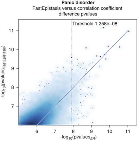
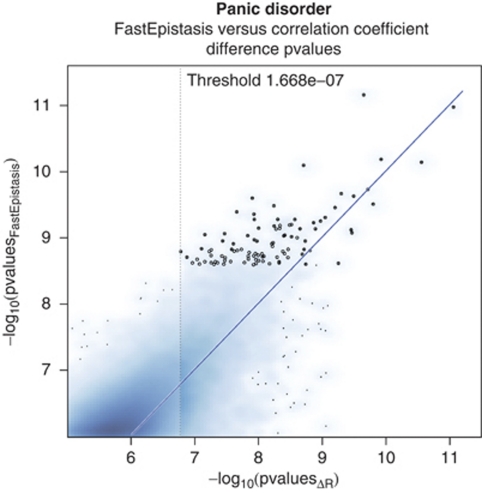
The results from SNP pairs with P-values below 1 × 10⁻⁶ tested against null from FastEpistasis are matched with the results obtained from the first stage of EPIBLASTER. From the panic disorder analysis, FastEpistasis produced 37336 SNP pairs, of which 36056 are also found in the EPIBLASTER stage 1 retained subset (96.5%). The unmatched pairs are indeed examples in which EPIBLASTER stage 1 underestimates the P-values and the hard threshold prevents it from being included. Thus, these unmatched pairs are all in fact situated around the P-values threshold region and are of lesser significance compared with the others. The plot of the matching pairs is shown in Figure 4, and for ease of visualization, it is illustrated as a smoothed color density of the actual scattered points plot. The top 10 most significant pairs from the FastEpistasis approach are listed with greater details in Table 1, along with their annotations in Table 2, and are marked with a dark circle in Figure 4. For EPIBLASTER stage 1 to capture all top 10 pairs of the ‘true' approach (FastEpistasis), a P-value threshold of 1.26 × 10⁻⁸ must be applied, thus resulting in the top 387 pairs of EPIBLASTER stage 1 to be passed onto stage 2. In other words, EPIBLASTER would have produced an additional 377 pairs to be tested in view of capturing the very top 10 true results. In Figure 5, the top 100 SNP pairs of the panic disorder study are marked, which would have resulted in applying a retention threshold for EPIBLASTER stage 1 of 1.67 × 10⁻⁷ passing on ∼5194 pairs to stage 2 (listed in greater detail in Supplementary Table 1).

Figure 4.

Panic disorder logarithmic P-values density plot: top 10 SNP pairs (points marked in black) and threshold correlation coefficient difference P-value. FastEpistasis P-values are on the y-axis, P-values from EPIBLASTER are on the x-axis.

Table 2. Top panic disorder SNP pairs annotations.

Top10 panic disorder SNP pairs ranked by FastEpistasis annotations
SNP1 name	Chromosome	Basepair	Gene	SNP2 name	Chromosome	Basepair	Gene
rs4653309	chr1	37876927		rs17338700	chr2	33841677
rs4984422	chr15	94456392		rs1967113	chr18	26830011	DSC3
rs1156847	chr9	2586783		rs7246846	chr19	56705171
rs6455842	chr6	162962566	PARK2	rs265548	chr19	17763334
rs12188192	chr5	136380739	SPOCK1	rs1317584	chr6	12450775
rs2100807	chr3	117506680	LSAMP	rs4875302	chr8	4028885	CSMD1
rs11900448	chr2	149650765	LOC130576	rs11939830	chr4	157150631
rs6762261	chr3	136073828	EPHB1	rs4745430	chr9	77461845
rs2374344	chr2	41994977		rs1011308	chr9	72478076
rs11925795	chr3	178001610		rs4731772	chr7	130582931

Figure 5.

Panic disorder logarithmic P-values density plot: top 100 SNP pairs (points marked in black) and threshold correlation coefficient difference P-value. FastEpistasis P-values are on the y-axis, P-values from EPIBLASTER are on the x-axis.

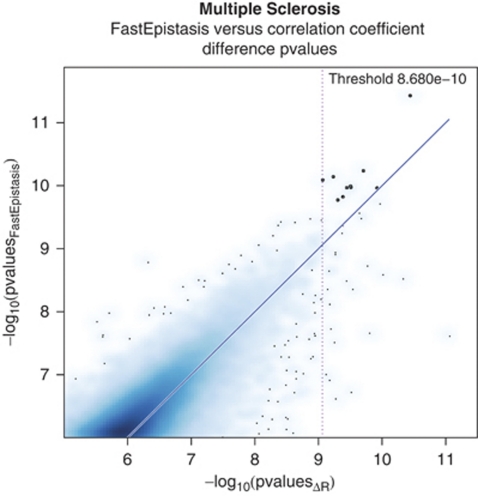
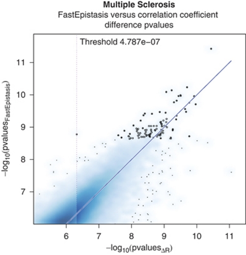
From the multiple sclerosis analysis, FastEpistasis yielded 42 731 pairs to have an interaction term with a P-value below 1 × 10⁻⁶, of which 42 524 pairs (99.5%) are also retained from EPIBLASTER stage 1. The matching pairs, along with the respective P-values tabulated using the FastEpistasis method versus the approximated EPIBLASTER stage 1 method, are plotted in Figure 6. The top 10 pairs are marked in Figure 6 and listed in Table 3, along with the SNP annotations in Table 4. For EPIBLASTER to capture the top 10 pairs, it would have required 48 of its top significant SNP pairs to be carried over to stage 2, where the P-values from logistic regression are tabulated. In addition, to capture the top 100 pairs, refer to Figure 7 (listed in greater detail in Supplementary Table 2). EPIBLASTER would have required the top 19 242 pairs obtained from stage 1 to be passed on to stage 2.

Figure 6.

Multiple sclerosis logarithmic P-values density plot: top 10 SNP pairs (points marked in black) and threshold correlation coefficient difference P-value.

Table 3. Top 10 multiple sclerosis SNP pairs difference of correlation coefficient, FastEpistasis and logistic regression P-values.

Top 10 multiple sclerosis SNP pairs ranked by FastEpistasis
Ranking	SNP1 name	SNP2 name	Difference of R	Difference of R P-value	FastEpistasis P-value	Lreg-SNP1 P-value	Lreg-SNP2 P-value	Lreg-interaction P-value
1	rs1392773	rs1384731	0.35723	3.68E-11	3.78E-12	7.00E-01	9.90E-01	4.28E-12
2	rs1552621	rs6817936	0.34409	2.00E-10	5.87E-11	7.85E-01	6.75E-01	6.71E-11
3	rs11710441	rs13226149	−0.33441	5.92E-10	7.28E-11	4.79E-01	2.21E-01	8.66E-11
4	rs2218314	rs1384731	0.33107	8.68E-10	8.19E-11	6.11E-01	9.99E-01	9.34E-11
5	rs6738313	rs3752735	−0.33932	3.18E-10	1.03E-10	1.91E-01	7.18E-01	1.12E-10
6	rs7593466	rs11658318	0.34033	3.14E-10	1.07E-10	7.66E-01	1.83E-01	1.01E-10
7	rs6758449	rs10055397	0.33889	3.64E-10	1.09E-10	3.23E-01	6.90E-01	1.16E-10
8	rs17648731	rs7386137	0.34748	1.22E-10	1.10E-10	8.15E-01	6.03E-01	1.05E-10
9	rs6550306	rs10503253	0.33773	4.17E-10	1.52E-10	9.32E-01	3.58E-01	1.66E-10
10	rs2542509	rs2916433	0.33511	5.04E-10	1.71E-10	6.94E-02	9.53E-01	1.81E-10

Table 4. Top 10 multiple sclerosis SNP pairs annotations.

Top10 multiple sclerosis SNP pairs ranked by FastEpistasis annotations
SNP1 name	Chromosome	Basepair	Gene	SNP2 name	Chromosome	Basepair	Gene
rs1392773	chr4	143053312		rs1384731	chr5	10660797
rs1552621	chr3	67460533		rs6817936	chr4	167934823	SPOCK3
rs11710441	chr3	145154009		rs13226149	chr7	94863536	PON3
rs2218314	chr4	143031581		rs1384731	chr5	10660797
rs6738313	chr2	3382368	TTC15	rs3752735	chr18	49363018
rs7593466	chr2	208807724	IDH1	rs11658318	chr17	27230172	UTP6
rs6758449	chr2	68290612	PPP3R1	rs10055397	chr5	120950796
rs17648731	chr2	77575007		rs7386137	chr8	142596655
rs6550306	chr3	34873129		rs10503253	chr8	4168252	CSMD1
rs2542509	chr2	71443251	ZNF638	rs2916433	chr4	4343724	LYAR/ZNF509

Figure 7.

Multiple sclerosis logarithmic P-values density plot: top 100 SNP pairs (points marked in black) and threshold correlation coefficient difference P-value.

Discussion

Although the search is conducted across all possible pairwise SNP interactions, the main interest is to delineate interactions between unlinked loci that influence the illness. In the first stage, the difference of Pearson's correlation coefficients, tabulated from the SNP pair, is taken between controls and cases across all possible interactions. In addition, this step can also incorporate replicating for significant association across two or more independent studies using a number of subjects' weighted meta-analysis during the actual run. In the current experimental setup with a genome-wide analysis of epistasis study, this first stage involving the difference of correlation coefficient evaluations can be completed within roughly 24 h on commercially available GPU setups compared with roughly a year on a single-core CPU. From the subset of interactions deemed significant in the rapid filtering stage, a second-stage analysis is performed using the likelihood ratio statistical test on the logistic regression to obtain the P-value on the estimated coefficients corresponding to the intercept, individual effects of the single loci and the interaction terms. As this necessitates only a minor amount of computations of logistic regressions in R using the ‘Anova' test on the ‘glm' fit with the ‘binary' family option, for a retention rate of 6.8 × 10⁻⁶, an expected 8.5 × 10⁶ pairs, this requires ∼2.5 days on a single core system of the hardware specifications listed in the methods section in R. This is impractical, however, if we are to limit ourselves to a range of top significant pairs that can be below a more stringent threshold, for example, 1.0 × 10⁻⁸, it drops down to an expected number of ∼600–700 pairs, which require around 150 s (four computations per second) to validate. It should be noted that dedicated software, such as INTERSNP (http://intersnp.meb.uni-bonn.de),⁹ is considerably faster for this second pass than pure R. The quoted figure of 8.5 × 10⁶ interaction pairs should be achieved between 1 or 2 hours using INTERSNP. A complete genome-wide association analysis with INTERSNP on a single core would be in the order of a year. FASTEPISTASIS would have taken ∼70 days on a single core. Note that INTERSNP is quoted here for a full logistic regression, whereas FASTEPISTASIS has a linear regression. Of course the performance of both INTERSNP (which again is about two orders of magnitude faster than plain R (using the glm() function)) and FASTEPISTASIS can be easily improved using multicore systems and clusters.

Of course, including more SNPs into the second stage is feasible. We have found a threshold of 6.8 × 10⁻⁶ practical. Lowering this by, for example, one order of magnitude will incur only a slight increase in runtime for stage 1 and a linear increase for stage 2. Of course, if the threshold for entry into stage 2 is lowered too much, hardware specifics such as disk speed become an issue in the performance of the program.

The reasoning behind the two-stage approach is threefold. First, the computations involved in the first stage are much less extensive as compared with estimating for significance in logistic regression. Second, a readily available R package, ‘gputools', allows the estimation of correlation coefficients to be performed on the graphic card, which greatly reduces the time and cost. Third, contrary to common multistage practice, in which the single locus test is performed initially, followed by higher order testing on loci that showed single locus significance, the necessity of interaction loci to first show significant marginal effects is not imposed, thus rendering this method a truly exhaustive search across all two-way interactions. The results from the MS and panic disorder analyses are used as the preliminary basis in cases in which this statement can be founded. A Plink method to test for univariate SNP significance is used to provide an indication of the SNPs that would be kept using the more traditional mandatory main effect significance. First, referring to Supplementary Tables S.2 and S.3 in the supplementary section, it is shown that a vast majority of significant interaction pairs would not have been captured if one is to prefilter based on univariate significance. Furthermore, referring to Supplementary Figures S.2–S.5 in the supplementary section, univariate P-values are plotted against the interaction pairs captured by EPIBLASTER. The lack of trends helps to support the fact that the method indeed conducts the search unbiased to the marginal effects at the two loci. High overestimation of the significance of the pair in the preliminary step 1 filtering stage can occur when the SNPs are very rare. Severe underestimation of P-values using this approximation (false negatives) has also rarely been noticed but was traced to a small subset of those SNP pairs that are in high linkage disequilibrium, which are not the main focus of this method. For computational ease, no lower bound on physical distance between SNPs or on LD between SNPs is imposed.

We also noted no inflation of the test statistic in our data sets; however, in certain cases it might be advisable to include MDS or PCA components in the analysis; for example, by working on residuals of the SNP genotypes on these components.

Overall, a comparison of the P-values obtained from FastEpistasis to the approximated P-values tabulated from EPIBLASTER stage 1 shows that, although discrepancy in P-values does exist, the adopted method does manage to capture all of the significant pairs, and the occurrence of significant pairs being omitted is practically nil when the threshold P-values are chosen to be far enough from the Bonferroni-corrected global significance. Nevertheless, the computational load for the second-stage analysis is negligible.

The concept of adopting the analysis of the difference of case-only and control-only studies into a unified test has been suggested in previous studies analyzing pairwise SNPs. Hoh and Ott¹⁰ initially proposed taking the ratios of the Chi-squares of the 3 × 3 contingency tables between cases and controls as a measure of significance. Zhao et al¹¹ and Zaykin et al¹² have also proposed examining the gene interactions with a defined linkage disequilibrium created by the interaction between two unliked loci. Significance is evaluated with the analysis of the difference of the LD values between case-only and control-only populations. Hardy–Weinberg equilibrium must hold for this measure of interaction and test statistics to be valid. Zhao et al has further suggested that the method exhibits greater power than conventional linear regression, as it does not treat the interaction as a residual term and allows for implicit nonlinear interaction and faster computational time than the traditional four degrees of freedom logistic regression model, rendering it more suitable for GWAS. The proposed method in this paper conducts the search in the first stage for only the effects of the interaction term by analyzing the difference of the correlation coefficients as an indication for significance, and then adopts the more conventional logistic regression method to substantiate the findings on a subset of pairs. As the difference is based on two separate groups, population stratification can have an effect on the power of the method. However, considering the number of pairs retained from our examples, the actual inflation is very low. In the multiple sclerosis analysis, 423 680 pairs are expected to be below the 1 × 10⁻⁵ threshold; an observed number of pairs captured is noted as 407 660. The method can indeed be simplified to a case-only study, by making the assumption that the correlation coefficient of the controls be null for all pairs. This approach would further speed up the computational time by a factor of 2 at the expense of potentially losing both power and precision. Moreover, the approximation approach does not only apply to the dosage coding (0, 1, 2), and also to other coding such as dominance, recessivity and heterozygosity. In general, a P-value cutoff of less than 1 × 10⁻⁵ should indeed be sufficient to capture all the results with a P<1 × 10⁻⁸ in the logistic regression and is, with all caution, suggested as a cutoff to be used in a first analysis, truly making EPIBLASTER exhaustive within this setting.

With respect to the results from MS and panic disorder that are presented, we note that, although there is no pair beyond a Bonferroni-corrected threshold for significance at a corrected P-value of 0.05, the marginal effects in the top 10 pairs do not at all show a tendency to deviate from a uniform distribution. This means that prefiltering pairs of SNPs on marginal P-values for subsequent epistasis analysis may be a less promising strategy than sometimes considered, although more analyses and larger sample sizes will be needed for a better founded statement on this issue.

In the editing phase of this article, it has come to our attention that Hu et al¹³ have also developed a strategy involving GPUs to enhance genome-wide significant SNP pair interaction search, quoting a total runtime of 27 h to scan through the Wellcome Trust Case Control Consortium's bipolar disorder data consisting of 500K SNPs. The proposed algorithm by Hu et al helps consolidate the improved time performance using the inherent parallel nature of GPU to search for significance in all possible SNP pairs. This method is distinct from ours as it uses the a difference of odds ratios measure between cases and controls to pick significant SNP pair candidates.

We would like to point out that with EPIBLASTER it is possible to perform genome-wide analysis of epistasis on very small-scale and inexpensive hardware, reducing the need for large clusters for this kind of application.

Future work is planned to incorporate the logistic regression and other more novel definitions of gene–gene interactions onto the graphical processing units. EPIBLASTER is available at http://www.mpipsykl.mpg.de/epiblaster.

The authors declare no conflict of interest.

References

- Marchini J, Donelly P, Cardon LR. Genome-wide strategies for detecting multiple loci that influence complex diseases. Nat Genet. 2005;37:413–417. doi: 10.1038/ng1537. [DOI] [PubMed] [Google Scholar]
- Wellek S, Ziegler A. A genotype-based approach to assessing the association between single nucleotide polymorphisms. Hum Hered. 2009;67:128–139. doi: 10.1159/000179560. [DOI] [PubMed] [Google Scholar]
- Gretton A, Borgwardt K, Rasch B, Schölkopf B, Smola A. A kernel method for the two-sample-problem. NIPS. 2006. pp. 513–520.
- R Development Core Team R: A language and environment for statistical computing Vienna, Austria: R Foundation for Statistical Computing; 2009. ISBN 3-900051-07-0, , http://www.R-project.org . [Google Scholar]
- Buckner J, Wilson J, Seligman M, Athey B, Watson S, Meng F. The gputools package enables GPU computing in R. Bioinformatics. 2010;26:134–135. doi: 10.1093/bioinformatics/btp608. [DOI] [PMC free article] [PubMed] [Google Scholar]
- Erhardt A, Czibere L, Roeske D, et al. TMEM132D, a new candidate for anxiety phenotypes: evidence from human and mouse studies Mol Psychiatry 2010. e-pub ahead of print 6 April 2010; doi: 10.1038/mp.2010.41 [DOI] [PubMed]
- Nischwitz S, Cepok S, Kroner A, et al. Evidence for VAV2 and ZNF433 as susceptibility genes for multiple sclerosis. J Neuroimmunol. 2010;227:162–166. doi: 10.1016/j.jneuroim.2010.06.003. [DOI] [PubMed] [Google Scholar]
- Schüpbach T, Xenarios I, Bergmann S, Kapur K. FastEpistasis: a high performance computing solution for quantitative trait epistasis. Bioinformatics. 2010;26:1468–1469. doi: 10.1093/bioinformatics/btq147. [DOI] [PMC free article] [PubMed] [Google Scholar]
- Herold C, Steffens M, Brockschmidt F, Baur MP, Becker T. INTERSNP: genome-wide interaction analysis guided by a priori information. Bioinformatics. 2009;25:3275–3281. doi: 10.1093/bioinformatics/btp596. [DOI] [PubMed] [Google Scholar]
- Hoh J, Ott J. Mathematical multi-locus approaches to localizing complex human trait genes. Nat Rev Genet. 2003;4:701–709. doi: 10.1038/nrg1155. [DOI] [PubMed] [Google Scholar]
- Zhao J, Xiong M. Test for interaction between two unlinked loci. Am J Hum Genet. 2006;79:831–845. doi: 10.1086/508571. [DOI] [PMC free article] [PubMed] [Google Scholar]
- Zaykin DV, Meng Z, Ehm MG. Contrasting linkage-disequilibrium patterns between cases and controls as a novel association-mapping method. Am J Hum Genet. 2006;78:737–746. doi: 10.1086/503710. [DOI] [PMC free article] [PubMed] [Google Scholar]
- Hu X, Liu Q, Zhang Z, et al. SHEsisEpi, a GPU-enhanced genome-wide SNP-SNP interaction scanning algorithm, efficiently reveals the risk genetic epistasis in bipolar disorder. Cell Res. 2010;20:854–857. doi: 10.1038/cr.2010.68. [DOI] [PubMed] [Google Scholar]
Associated Data
This section collects any data citations, data availability statements, or supplementary materials included in this article.