Abstract
A system of ordinary differential equations describes the populuation dynamics of a rabies epidemic in raccoons. The model accounts for the dynamics of vaccine, including loss of vaccine due to animal consumption and loss from factors other than racoon uptake. A control method to reduce the spread of disease is introduced through temporal distribution of vaccine packets. This work incorporates the effect of the seasonal birth pulse in the racoon population and the attendant increase in new-borns which are susceptible to the diseases, analysing the impact of the timing and length of this pulse on the optimal distribution of vaccine packets. The optimization criterion is to minimize the number of infected raccoons while minimizing the cost of distributing the vaccine. Using an optimal control setting, numerical results illustrate strategies for distributing vaccine depending on the timing of the infection outbreak with respect to the birth pulse.
Keywords: rabies epidemic model, vaccine, optimal control, ordinary differential equations
1. Introduction
Rabies is a common RNA virus that is transmitted within wildlife causing death to an infected organism after a given incubation period. This virus is a member of the genus Lyssavirus of the family Rhadbdoviridae, and order Mononegavirales [12, 25]. Since the development of an oral rabies vaccine (ORV) for wildlife, attention has been focused on the strategic use of vaccination to contain the spread of rabies.
Today, raccoons have been identified as the most common terrestrial wildlife host of the rabies virus in the eastern United States [12]. Prior to 1998, efforts to control rabies spread was carried out on a state-by-state basis. Control efforts are based on the distribution of ORV baits. Each bait is a plastic package containing the vaccine and coated with fish meal and oil. The vaccine packets are frequently dropped from airplanes flying above a given region inhabited by wildlife [2, 19, 22]. Raccoons are vaccinated by ingesting the vaccine as they consume the fish meal coating [11]. In 1998 federal funds were made available to to the US Department of Agriculture, Animal and Plant Health Inspection Service to create a national program to coordinate and enhance rabies control efforts across state agencies [22]. Under this program state-level bait distribution programs were integrated to create a vaccination corridor to contain raccoon-rabies within the eastern US. The vaccination corridor extends southern Canada southward to the Gulf coast [25]. However, the timing of bait delivery within the vaccine corridor is chosen on an ad-hoc basis. In addition, the cost of rabies vaccination is high. In 1996, the reported cost of programs designed to contain the spread of infection exceeded $300 million. In this paper we develop a mathematical model that provides quantitative insights into the trade-offs between the timing and cost of vaccination.
Ordinary differential equations (ODEs) as well as partial differential equations (PDEs) have been used to model the dynamics of populations that contain the rabies virus. Murray, et. al. used ODEs to study the dynamics of susceptible and infected foxes in Europe coupled with a PDE describing the dispersal of the rabid class [16]. This paper also discussed various vaccination and culling strategies. In a later paper, an immune class was included affecting the behavior of periodic outbreaks associated with oscillating tail of the epidemic wave [15]. Evans and Pritchard extended Murray’s 1986 model to include a vaccinated class of foxes with the goal of controlling the density of the infected population to be below a predetermined number [6]. An ODE model developed by Coyne et. al., divided raccoons into six categories: susceptible, exposed, infected, rabid, naturally immune, and vaccinated [4]. The results of this research showed the the least expensive control strategy involved exclusively either culling or vaccination. A combined approach is cheaper only when the per capita cost of vaccination is less then 20% of the per capita cost of culling.
A stochastic spatial model developed by Smith, et. al. described the spread of rabies in Connecticut [23]. Results from this model suggest rivers act as a semipermeable barrier to the spread of rabies resulting in a seven fold reduction in the rate of spread. A reanalysis of the Connecticut data considered the influence of habitat and long-distance translocation events [24]. The results of the reanalysis suggest that rivers interact with the degree of forest cover to further reduce the spatial spread of raccoon rabies [24]. The model results also suggest that long-distance translocation events do not produce new foci of infection [24]. The stochastic model used in these analyses is based on a spatial network defined by the locations of townships within Connecticut [23]. Townships are categorized as either undocumented or infected and the spread of infection was represented as a transition from the undocumented class to the infected class. This stochastic spatial model was used by Russell et. al. to analyze data from Ohio [21]. In 2004 rabies was detected in Lake County Ohio and the model results suggested that rabies would spread across Ohio in as little as 36 months [21]. Members of this team later authored another paper using an ODE model to show that the spread of rabies may be controlled by distributing vaccine behind barriers such as rivers [20].
Asano et al. first applied optimal control to a system modeling an infected raccoon population [2]. This SIR model included the three classes in 9 spatial compartments giving a total of 27 ODEs. Results showed that a higher rate of vaccination is needed for a larger population but a lower distribution of vaccine given a high cost. Recently, Ding et al. investigated the distribution of vaccine baits in a rabies epidemic in raccoons, with a model, discrete in time and space [5]. The results showed that distribution of vaccine depended on the location of the rabies infection. If the virus is detected in the middle of a patch, vaccine is applied heaviest to the center of the spread of infection. If the infection is observed in a corner of a patch, the distribution of the vaccine is given around the edges to prevent the spread of the infection.
In some raccoon populations, mating and parturition only occur during specific times of the year [9]. A more realistic model could include a ‘birth pulse’ where organisms are added to a population during a specific time interval. Many models use the term ‘pulse’ to mean the population has a discontinuous jump at a particular time [8, 18, 26]. Here the population is continuous in time with an expected increase in animals for a period of time during the year; the increase comes from a step function pulse in the derivative.
An important new feature of this work is the investigation of the effects of a birth pulse on the timing of vaccine delivery through the analysis of a pulsed system of ODEs. One of the conclusions will show that the distribution of the vaccine depends on the time that the rabies infection is detected relative to the birth pulse. The closer the detection is to the time of the seasonal births, the longer the distribution of vaccination must be sustained. Our approach uses optimal control strategies for a model system that includes the dynamics of the vaccine. Including a dynamic equation for the level of the vaccination is another novel feature. The goal is to find optimal strategies for distributing vaccine packets to minimize the size of the infected population and the cost of implementing the control. The effect of the birth pulses on this strategy is investigated.
The basic model is introduced in the next section followed by a discussion of the dynamics of the vaccine. Then we describe the existence of solutions for the corresponding adjoint system and an optimal control. Numerical results are reported in section 3 for various scenarios with section 4 considering the possibility of having a limited amount of vaccine available for distribution. We conclude with a summary and interpretation of the numerical simulations.
2. The Epidemic Model with Vaccine Dynamics
Various kinds of seasonal forcing have been shown to influence biological systems with infectious diseases [1, 10]. The periodic effect of annual birth pulses is a kind of forcing that occurs at the same time each year. It is assumed that raccoons give birth during the spring time of the year, March 20 – June 21. For a 365 day year starting from January 1, we have March 20 as day 79 and June 21 as day 172. The entire birth pulse is 93 days. There are four classes of raccoons, S susceptibles, E exposed, I infecteds, and R immune, in this model. The system of ordinary differential equations also includes the dynamics of the amount of vaccine available:
| (1) |
where V is the amount of the vaccine at time t and the control u is the rate of vaccine distribution. The birth pulse occurs on the set , tk = 79 + 365k and tk+1 = 172 + 365k.
Any raccoon that can transmit the rabies virus, will be in the infected class, designated as I. A population of raccoons that does not have the rabies virus but has the potential to contract the disease will be called susceptible and is identified as S. When a susceptible becomes exposed to the rabies virus, an incubation period occurs during which time the raccoon does not immediately have the ability to transmit the disease but is only a latent carrier of the disease. The average time of this incubation period is 1/a. This class will be called exposed and represented as E. The interaction between the susceptible and exposed classes is expressed symbolically as βIS where βIS is the rate that a member of the susceptible class becomes infected.
It is assumed that a small percentage of exposed raccoons will develop a natural immunity to the rabies virus, designated 1 − ρ, where ρ is the percentage that die from the disease. This phenomenon introduces a new class called the immunes, R.
The per-capita birth rate per day is a during the birth pulse. During the spring, the S, E, R classes are able to give birth, and the birth rate is represented symbolically as
where χ(t)[t0,t1] is a characteristic function with t0, t1 corresponding to March 20 and June 21, respectively. All births enter the susceptible class. Raccoons die of non-rabies causes at a per-capita rate per day of b. The total population at any time is N = S + E + R + I with a dynamical equation of
If vaccine baits are introduced into the environment, it is assumed that they are eaten by the susceptible raccoons with a conversion rate to the immune class as . This term gives a saturation effect due to the foraging of raccoons from the baits. The constant K is a “half-saturation” constant, the value of V such that becomes . The vaccine baits are depleted by being eaten by the raccoons, other wildlife or natural decay. The rate at which the baits are eaten by S, E and R, is c. Otherwise, the baits are eliminated at a rate of c1 due to other causes, like natural decay or consumption by other animals. The control u is the rate of vaccine distribution.
Since the right hand sides of the state equations are measurable in t and continuous in the state and control variables, there exist a solution to the system by Theorem 9.2 of [14]. The structure of the systems gives that when E(0) = R(0) = V(0) = 0, and S(0) and I(0) are positive, all the state variables are positive throughout the time interval. Note that since all the state variables are non-negative for all t ≥ 0, then N′ ≤ aN implies the boundedness of N(t) for any finite time interval. Thus all the state variables are also bounded.
To minimize the infected population as well as the cost of the vaccine, the objective functional is
The set of all admissible controls is
where M1 is a positive constant and the upper bound of u. The coefficient A converts the number of infected raccoons into a cost. If we divide the objective functional by A, we will obtain the same optimal control. So the rate would be the crucial parameter, and thus we take A = 1. The cost coefficient B is a weight factor balancing the two terms. When B is large, then the cost of implementing the control is high. We seek to find u* in U such that
Using a standard existence result from [7], there exists an optimal control u* ∈ U which minimizes the objective functional J(u).
To use Pontryagin’s Maximum Principle [17], we form the Hamiltonian, grouped in terms of u
| (2) |
Theorem 2.1
Given an optimal control u and the corresponding state solutions S, E, I, R and V, there exist adjoint functions λ1(t), λ2(t), λ3(t), λ4(t), λ5(t) satisfying the adjoint system:
| (3) |
with λi(T) = 0, for each i, and
| (4) |
where the singular control is given by
| (5) |
provided 0 ≤ us ≤ M1.
Furthermore the generalized Legendre Clebsch condition is satisfied for this singular control giving necessary conditions when the optimal control is singular.
Proof
Suppose u is an optimal control and S, E, I, R, V are corresponding state solutions. Using the result of Pontryagin’s Maximum Principle [17], there exist adjoint variables λ1(t), λ2(t), λ3(t), λ4(t), λ5(t) satisfying
| (6) |
The behavior of the control may be obtained by differentiating the Hamiltonian with respect to u, giving at time t,
For this minimization problem, we use the sign of that partial derivative to obtain part of the control characterization:
Next we consider the singular case. If Hu = 0 on some non-empty open interval of time, say (a1, b1), then
Substitution into the respective adjoint equation and rearranging gives
| (7) |
Since c1 is positive and the state variables are positive, equation (2.9) implies
Differentiating with respect to t yields
| (8) |
Substituting for V′ gives
Since on (a1, b1), solving the above equation for u,
Substitution for S′ + E′ + R′ and into the expression for u with λ5 = −B,
| (9) |
Grouping terms, the singular control is:
| (10) |
Since λ5′ does not contain any u terms and λ5″ does contain u, this singular control has order 1.
The generalized Legendre Clebsch condition [13] in a minimization problem with a singular control of order 1 is a necessary condition for the singular control to be optimal. Our model has a singular control of order 1 and satisfies the generalized Legendre Clebsch condition:
3. Numerical Results
Values of the below parameters are based on the non-control case in [4, 21, 23, 24]. The parameters pertaining to the populations are
birth rate (constant per-capita)
death rate (constant per-capita)
average time raccoon spends infectious
βI = 0.01I infection rate
average time from infection until raccoon is infectious or recovers
ρ = 0.98 fraction that die from rabies
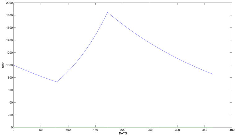
The death rate b was chosen to maintain a disease free population near the initial condition for a period of one year. Figure 1 displays a graph of the population dynamics of raccoons for a duration of 1 year without interaction with the rabies virus starting from an initial population of 1000, i.e. S0 = 1000. This disease free case can be solved explicitly by considering S′ = (aχΩ − b)S with solution, S(t) = S(0)e−btea[t1−t0], when t1 ≤ t ≤ 365. A sustainable population is achieved when a[t1 − t0] − bt = 0. For t = 365 and t1 − t0 = 93, we obtain . If the birth rate a = 0.006, then the death rate b ≈ 0.0015.
Figure 1.
One year projection of disease free raccoon population starting on January 1
Parameters related to the vaccine are:
, rate of vaccination of S
c1 = 0.01, rate at which baits decay
c = 0.01, rate at which baits are eaten by S, E, R
K = 1.0, half-saturation level
The numerical results involving the optimal control below were obtained using an iterative method with a 4th-order Runge-Kutta scheme programmed in Matlab to solve the optimality system. Starting with the initial conditions S0, E0, I0, R0, V0 and an initial guess for the control, forward sweeps with the Runge-Kutta scheme were used to obtain approximate solutions for the state equations. Using those state values, the solutions of the adjoint equations were approximated using backward sweeps from the final time condition, λ1(T) = λ2(T) = … = λ5(T) = 0. The control is updated using the control characterization. Iterations continue until convergence occurs, i.e., successive values of all variables from current and previous iterations are sufficiently close. To help justify the bang–bang feature of the control, |λ5 + B| was used to verify the output of the control variable. But in our numerical results, the singular case does not occur. Note that the upper bound of the control is taken to be 1. Large upper bounds were also used given similar results in patterns, but with a small number of days of distribution.
In response to an outbreak that is detected, there will in general be a rapid response of public health agencies to limit the potential spread of the disease. We therefore focus here on numerical examples on short-term response solutions using a duration of 28 days. A longer period of analysis could readily be analyzed using the same methods. Due to the short time period used in these reults, we do include immigration or emigration effects. We take the geographic area under consideration as 100 km2 with initial populations of 1000 susceptibles and 40 infecteds, i.e., S0 = 1000, I0 = 40. It is also assumed that no exposed or immunes are initially present.
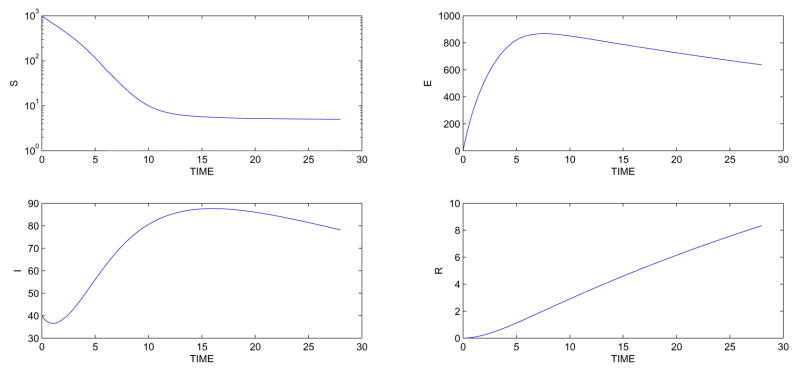
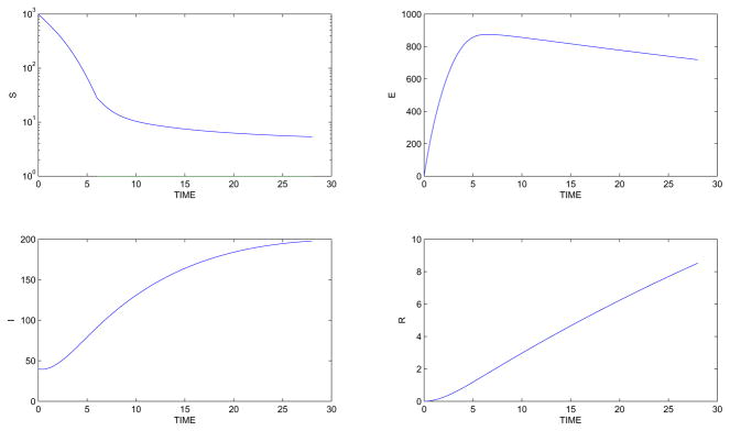
With the same initial number of susceptibles, we now introduce 40 infected raccoons on March 14, the 73th day of the year. The time period begins on March 14 for a duration of 28 days with the birth pulse starting on March 20 (which is the 7th day of this period). Since without any control the susceptibles quickly decrease in number, a logarithmic scale is used for the susceptibles in order to observe the effect of the pulse. Figure 2 shows the susceptibles quickly moving into the exposed class and the number of infecteds doubling approximately 12 days into the interval. Note the relatively small number in the immune class arising from the low rate assumed for natural immunity.
Figure 2.
State variables with disease and no control: Simulation begins on March 14.
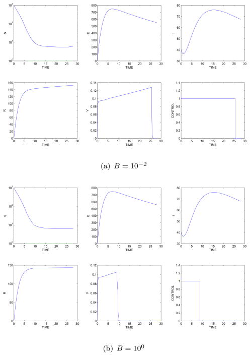
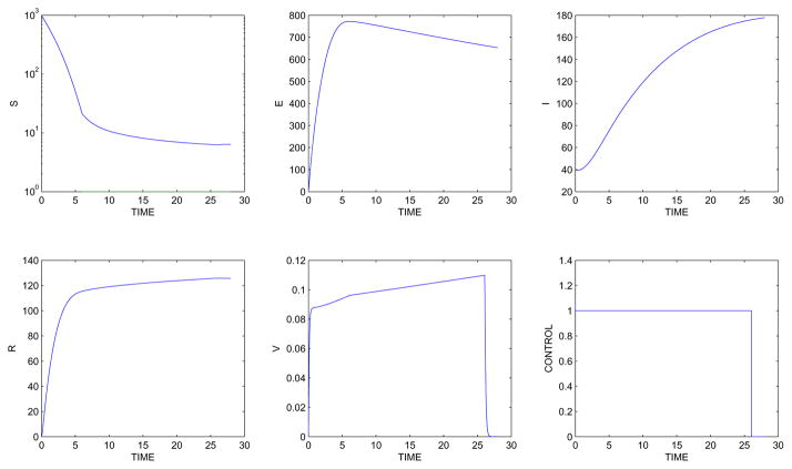
When vaccine and the associated cost are included in the optimal control problem, the immune class increases due to the vaccination strategy. For example, under the same starting day (March 14) and the same initial conditions S0 = 1000, I0 = 40, R0 = 0 = E0 and a cost coefficient B = 10−2, the optimal control u is at 1 during days 1 – 22, as seen in figure 3a. For a cost coefficient B= 100 and the same initial conditions, the control u is at 1 for days 1 – 9. The results are displayed in figure 3b. Thus less control is seen due to the higher cost.
Figure 3.
State variables with optimal control results for (a) B = 10−2, (b) B = 100: Simulation begin on March 14.
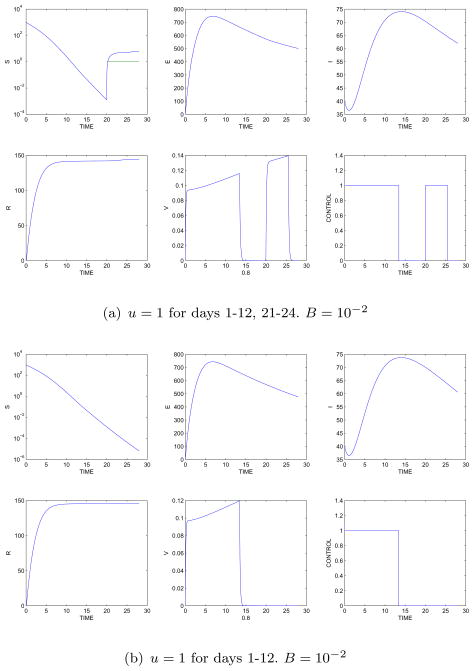
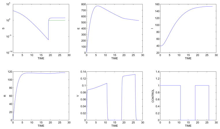
Various numerical solutions were carried out which varied the position of the start of the outbreak with respect to the birth pulse. Figure 4a shows the results if the 28 day interval begins on March 1 (which is 19 days before the birth pulse starts). In this case vaccine is distributed for 12 days after the infection is detected and then resumes at the beginning of the birth pulse and continues for March 21–25. This case illustrates the importance of considering policies with a second round of vaccine distribution following the start of the birth pulse. If the disease is detected a month before the birth pulse, then the optimal amount of vaccine is distributed for the first 12 days only (figure 4b). A second round of vaccination distribution is not needed in this case becuase the time period is constrained to be prior to the birth pulse.
Figure 4.
State variables with optimal control results with the 28 day interval:(a) beginning March 1. (b) beginning February 20.
To investigate the dependence of the results on parameters which are not well-determined and have a range of possible values [4, 21, 23, 24], additional simulations were made using the following:
a = 0.014/day birth rate (constant per-capita)
b = 0.004/day death rate (constant per-capita)
1/α = 1/0.07 average time raccoon spends infectious
Recall that for the disease free case, the susceptible differential equation is
with solution S(t) = S(0)e−btea[t1−t0] when t1 ≤ t ≤ 365. For t = 365 and t1 − t0 = 93, we obtain . If the birth rate a = 0.014, then the death rate b ≈ 0.004. Other parameters remained unchanged. Note that the maximum number of raccoons in a numerical simulation of a period without disease is significantly larger than with the old parameters.
Forty infected raccoons introduced into the susceptible population on March 14 (the 73th day of the year) for 28 days yields a greater number of infecteds across time. The results are displayed in figure 5.
Figure 5.
Under new parameters, state variables with disease and no control: starting on March 14.
With the new parameters in figure 6 and starting on March 14, more infected occur compared to the results of figure 3a with a cost coefficient of B = 10−2. The optimal controls are very similar. Now starting on March, figure 7 shows again a larger number of infected compared with figure 4a and show similar control results.
Figure 6.
State variables and optimal control results for new parameters when B = 10−2: beginning on March 14
Figure 7.
State variables and optimal control results with new parameter for B = 10−2: beginning March 1.
We also investigated numerical solutions for a model which included density dependence in the mortality. The terms, −bS, −bE, −bR, were replaced by −bS(S + E + R), −bE(S + E + R), −bR(S + E + R). The numerical results when density dependence of this form was included were very similar to the results shown here without density dependence. Thus although the exact quantitative values for the optimal control vary somewhat for different models for underlying population dynamics associated with mortality rates, the qualitative behavior of the optimal control solution is quite similar. Thus we surmise that if the demographics of the raccoon population are not known precisely, the optimal control results can still give a type of “rule of thumb” policy in terms of distribution of vaccine near the time of the birth pulse.
4. Limited Vaccine
In practical application, there is a limit to the resources available to carry out vaccination treatment. To include this aspect of realism, we modify the model by assuming a limited amount of vaccine is available for distribution. This is represented mathematically through the addition of an integral constraint on the control and may be included in the above model by introducing a new state variable z(t) such that
with z(T) = C, where C =constant. The new state equation is z′ = u, with boundary conditions z(0) = 0, z(T) = C. The Hamiltonian becomes
| (11) |
Since the objective functional is
where the set of controls is {u: [0, T] → [0, 1]|u is Lebesgue measurable}, the same adjoint equations above are included in the new system with the addition of
with no boundary conditions, since the new state variable z has two boundary conditions. The optimal control may be characterized similarly as in (4).
| (12) |
We completed numerical results in this case for the original set of parameters and illustrate based upon one set of parameters. The numerical algorithm requires another iteration due to the need to find the constant value of λ6, that gives the correct integral condition on u*. The target integral value was taken to be z(T) = 10 for the simulations below.
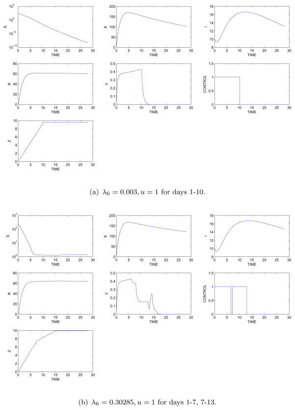
Figure 8 shows the results for an interval (a) with no birth pulse and for an interval (b) with the 28 day interval beginning on March 14 (which is 6 days before the start of the birth pulse b). The results show that the optimal control may be maintained during the first 10 days when no birth pulse occurs in case (a), but requires a brief cessation in the middle of case (b). Of course, when comparing these results to the previous cases with linear costs in the objective function, there are more or less days of vaccination in the optimal control depending on the cost parameter B.
Figure 8.
Population and control results with the integral constraint on the control: (a) 28 interval without a birth pulse. (b) 28 day interval beginning on March 14.
5. Conclusion
The models developed and analyzed here included several new aspects to incorporate more realistic assumptions about rabies spread in racoons, with emphasis on developing optimal control schemes to determine the “best” methods to constrain the spread of the disease once it is detected. The new components incorporated include an exposed class, an explicit birth pulse which occurs seasonally, and dynamics of the vaccine packets associated with uptake by racoons as well as loss due to other factors. The key results derived illustrate the dependence on the optimal timing of distribution of vaccine packets on the timing of disease detection relative to the birth pulse. While the exact optimal timing results vary with parameter assumptions, there are a number of general results which appear to be rather robust based upon the illustrations presented here and numerous other cases also investigated [3].
One general result concerns a type of “rule of thumb” arising from investigation of the effect of the birth pulse on the timing of vaccine delivery which may be useful in developing policies for vaccine distribution following an outbreak detection. If the infection is detected near start of the birth pulse, the optimal control distributes the vaccine immediately for a certain period of time. If the infection is detected a few weeks before the birth pulse, the optimal distribution of vaccine begins immediately, stops briefly and then resumes for a certain period of time. If the distribution starts at about March 1 or about 3 weeks before the start of the birth pulse, then under most situations (e.g. for most parameter sets investigated) a second round of vaccine distribution is optimal after the start of the birth pulse.
If the birth pulse occurs soon after the disease detection and the start of the vaccination distribution, the optimal treatment is necessary for a longer period of time. Thus if the disease were detected and distribution started at about March 14, more days of vaccine distribution are optimal than if the detection occured on an earlier date. The closer the detection of the rabies outbreak is to the start of the birth pulse, the longer the period of optimal distribution of vaccine is projected to be.
For other parameters fixed, the optimal number of days to distribute the vaccine decreases with higher cost. The general qualitative results noted above arise as well when costs are accounted for in a different manner, by assuming there is a fixed total amount of effort allowed on vaccine distribution. The qualitative behavior of optimal solutions appears to be robust relative to differing assumptions about vaccine distribution costs.
Our examples focused on a 28 day total duration for the control period. In this situation, the number of infecteds is never completely eliminated, but if the optimal policy for vaccine distribution is followed, more raccoons join the immune class and that number exceeds the population of the infected class. The period for which the optimal solution is calculated can readily be extended using the same methodology presented here, but in this case additional assumptions must be made about immigration and emmigration rates, which were ignored here due to the short duration of the time period considered. Sufficient input of new susceptibles due to immigration can effectively act as another ”birth pulse” however and thus if net immigration is positive over some extended time period, the effect would be similar to a longer birth pulse. If net immigration included infected or exposed individuals, then we expect that the period of optimal vaccine distribution would be lengthened, though we have not investigated this situation.
Taking account of different mortality assumptions, through inclusion of density-dependence in this model component, did not qualitatively change the nature of the optinal control solution for vaccine distribution. This robustness of the optimal solution for alternative model forms was only investigated for a few parameter sets however, so there may be situations in which alternative assumptions about mortality have larger qualitative impacts. Our results do provide some hope however that even if the exact demographic details of population dynamics are not well-specified, the general patterns of optimal control would still apply.
A major use of general models such as those presented here is to evaluate under simplifying assumptions what the “best” policies would be to limit disease spread. As such they also allow elaboration of how much “worse” the impact of the disease would be (measured for example in terms of total number of deaths resulting from disease over the chosen time horizon) if the policy chosen were off by a small or large amount from the optimal one (measured for example in terms of the period for which the vaccine is distributed). This is useful for policy decisions in which there are uncertainties about the details of demographics or transmission assumptions in that they can provide a basis for determining how much effort might be effectively devoted to either obtaining more accurate data (e.g. through surveillance methods) rather than expending effort on further vaccination. Expansion of the methods developed here to account for the trade-offs in expenditure for surveillance versus vaccination could well be a very important contributor to establishing policy decisions regarding wildlife infectious disease management.
Acknowledgments
This work was supported by National Science Foundation (NSF) Award IIS-0427471 to the University of Tennessee and National Institutes of Health (NIH) grant R01 AI047498 to LAR.
References
- 1.Altezer S, Dobson A, Hosseini P, Hudson P, Pascual M, Rohani P. Seasonality and the Dynamic of Infectious Diseases. Ecology Letters. 2006;9:467–484. doi: 10.1111/j.1461-0248.2005.00879.x. [DOI] [PubMed] [Google Scholar]
- 2.Asano E, Gross LJ, Lenhart S, Real L. Optimal Control of Vaccine distribution in a Rabies Metapopulation Model. Mathematical Biosciences and Engineering. 2008;5:219–238. doi: 10.3934/mbe.2008.5.219. [DOI] [PubMed] [Google Scholar]
- 3.Clayton TJ. PhD dissertation. University of Tennessee; 2008. Optimal cotnrol of epidemic models involving rabies and West Nile viruses. [Google Scholar]
- 4.Coyne MJ, Smith G, McAllister FE. Mathematic Model for the Population Biology of Rabies in Raccoons in the Mid-Atlantic States. American Journal of Veterinary Research. 1989;50:2148–2154. [PubMed] [Google Scholar]
- 5.Ding W, Gross LJ, Langston K, Lenhart S, Real L. Optimal Control of Vaccine Distribution in a Rabies Metapopulation Model. Journal of Biological Dynamics. 2007;1:379–398. doi: 10.1080/17513750701605515. [DOI] [PubMed] [Google Scholar]
- 6.Evans ND, Pritchard AJ. A Control Theoretic Approach to Contanining the Spread of Rabies. IMA Journal of Mathematics Applied in Medicine and Biology. 2001;18:1–23. [PubMed] [Google Scholar]
- 7.Fleming WH, Rishel Raymond W. Deterministic and Stochastic Optimal Control. Springer-Verlag; New York: 1975. [Google Scholar]
- 8.Gao S, Chen L, Sun L. Dynamic Complexities in a Seasonal Prevention Epidemic Model with Birth Pulses. Chaos Solitons and Fractals. 2005;26:1171–1181. [Google Scholar]
- 9.Gehrt SD. Raccoons and allies. In: Feldhamer GA, Chapman JA, Thompson BC, editors. Wild Animals of North America. John Hopkins University Press; 2003. pp. 1–15. [Google Scholar]
- 10.Greenman J, Kamo M, Boots M. External Forcing of Ecological and Epidemilogical Systems: A Resonance Approach. Physica D. 2004;190:136–151. [Google Scholar]
- 11.Hanlon CA, Rupprecht CE. The reemergence of rabies. In: Scheld WM, Armstrong D, Hughes JM, editors. Emerging Infections. ASM Press; Washington D. C: 1998. pp. 59–80. [Google Scholar]
- 12.Jackson AC, Wunner WH. Rabies. Academic Press; Boston: 2002. [Google Scholar]
- 13.Krener AJ. The High Order Maximal Principle and its Application to Singular Extremals. SIAM J Control and Optimization. 1977;15:256–293. [Google Scholar]
- 14.Lukes DL. Differential Equations: Classical to Controlled, Mathematics in Science and Engineering. Academic Press; New York: 1982. [Google Scholar]
- 15.Murray JD, Seward WL. On the Spatial Spread of Rabies Amoung Foxes with Immunity. J Theo Biol. 1991;130:327–348. [Google Scholar]
- 16.Murray JD, Stanley EA, Brown DL. On the Spatial Spread of Rabies Amoung Foxes. Proc R Soc London B. 1986;229:111–150. doi: 10.1098/rspb.1986.0078. [DOI] [PubMed] [Google Scholar]
- 17.Pontragin LS, Gamkrelize RV, Boltyanskii VG, Mishchenko EF. The Mathematical Theory of Optimal Processes. Wiley; 1962. [Google Scholar]
- 18.Roberts MG, Kao RR. The Dynamics of an Infectious Disease in a Population with Birth Pulses. Mathematical Biosciences. 1997;149:23–36. doi: 10.1016/s0025-5564(97)10016-5. [DOI] [PubMed] [Google Scholar]
- 19.Rupprecht CE, Hanlon CA, Slate D. Oral vaccination of wildlife against rabies: opportunities and challenges in prevention and control. Dev Biology. 2004;11(9):173–184. [PubMed] [Google Scholar]
- 20.Russell CA, Real LA, Smith DL. Spatial Control of Rabies on Heterogeneous Landscapes. PLoS ONE Dec. 2006;20:1–27. doi: 10.1371/journal.pone.0000027. [DOI] [PMC free article] [PubMed] [Google Scholar]
- 21.Russell CA, Smith DL, Childs JE, Real LA. Predictive Spatial Dynamics and Strategic Planning for Raccoon Rabies Emergence in Ohio. PLoS Biology. 2005;3:382–388. doi: 10.1371/journal.pbio.0030088. [DOI] [PMC free article] [PubMed] [Google Scholar]
- 22.Slate D, Rupprecht CE, Rooney JA, Donovan D, Lein DH, Chipman RB. Status of oral rabies vaccination in wild carnivores in the United States. Virus Research. 2005;111:68–76. doi: 10.1016/j.virusres.2005.03.012. [DOI] [PubMed] [Google Scholar]
- 23.Smith DL, Lucey B, Waller LA, Childs JE, Real LA. Predicting the Spatial Dynamics of Rabies Epidemics on Heterogeneous Landscapes. PNAS. 2002;99:3668–3672. doi: 10.1073/pnas.042400799. [DOI] [PMC free article] [PubMed] [Google Scholar]
- 24.Smith DL, Waller LA, Russell CA, Childs JE, Real LA. Assessing the Role of Long-Distance Translocation and Spatial Heterogeneity in the Raccoon Rabies Epidemic in Connecticut. Preventative Veterinary Medicine. 2005;71:225–246. doi: 10.1016/j.prevetmed.2005.07.009. [DOI] [PMC free article] [PubMed] [Google Scholar]
- 25.Smith J. New Aspects of Rabies with Emphasis on Epidemiology, Diagnosis, and Prevention of the Disease in the United States. Clinical Microbiology Reviews. 1996;9:166–176. doi: 10.1128/cmr.9.2.166. [DOI] [PMC free article] [PubMed] [Google Scholar]
- 26.Tang S, Chen L. Density-Dependent Birth Rate, Birth Pulses and their Population Dynamic Consequences. J Math Biol. 2002;44:185–199. doi: 10.1007/s002850100121. [DOI] [PubMed] [Google Scholar]


