Abstract
This paper uses a general latent variable framework to study a series of models for non-ignorable missingness due to dropout. Non-ignorable missing data modeling acknowledges that missingness may depend on not only covariates and observed outcomes at previous time points as with the standard missing at random (MAR) assumption, but also on latent variables such as values that would have been observed (missing outcomes), developmental trends (growth factors), and qualitatively different types of development (latent trajectory classes). These alternative predictors of missing data can be explored in a general latent variable framework using the Mplus program. A flexible new model uses an extended pattern-mixture approach where missingness is a function of latent dropout classes in combination with growth mixture modeling using latent trajectory classes. A new selection model allows not only an influence of the outcomes on missingness, but allows this influence to vary across latent trajectory classes. Recommendations are given for choosing models. The missing data models are applied to longitudinal data from STAR*D, the largest antidepressant clinical trial in the U.S. to date. Despite the importance of this trial, STAR*D growth model analyses using non-ignorable missing data techniques have not been explored until now. The STAR*D data are shown to feature distinct trajectory classes, including a low class corresponding to substantial improvement in depression, a minority class with a U-shaped curve corresponding to transient improvement, and a high class corresponding to no improvement. The analyses provide a new way to assess drug efficiency in the presence of dropout.
Keywords: Latent trajectory classes, random effects, survival analysis, not missing at random
Introduction
This paper considers growth modeling of longitudinal data with missingness in the form of dropout that may be non-ignorable. Non-ignorable missing data modeling acknowledges that missingness may depend on not only covariates and observed outcomes at previous time points as with the standard missing at random (MAR) assumption (Little & Rubin, 2002) customarily made in multivariate analysis software. Missingness may also depend on latent variables such as values that would have been observed (missing outcomes), developmental trends (growth factors), and qualitatively different types of development (latent trajectory classes). Many different missing data models for such situations have been presented in recent years, e.g. Albert and Follman (2009), Beunckens et al. (2008), Dantan et al. (2008), Little (2009), Roy and Daniels (2008), and Yuan and Little (2009). The proposed models use both continuous latent variables in the form of random effects and categorical latent variables in the form of finite mixtures. Because missing data models draw on untestable distributional assumptions about missing data it is important to do a sensitivity analysis using several different models. To this aim, this paper uses a general latent variable framework summarized in Muthén and Asparouhov (2009) to explore and compare a series of key models proposed in the literature as well as several new models. To illustrate the various models, analyses are performed on data from the trial Sequenced Treatment Alternatives to Relieve Depression (STAR*D). Comparisons of models on a given data set have been hampered by lack of software development for general missing data analyses, with software typically presented for only a few model variations considered in the authors’ article. The latent variable framework of Muthén-Asparouhov is implemented in the Mplus software (Muthén & Muthén, 1998–2010) which was used for all analyses in the paper. Estimation is carried out using maximum-likelihood using the EM algorithm as described in Muthén and Asparouhov (2009). Mplus scripts for the analyses are available at http://www.statmodel.com/examples/penn.shtml#stard.
STAR*D is the largest antidepressant clinical trial in the U.S. to date. Nevertheless, analyses using modern missing data techniques have not been performed until now. In the STAR*D data, latent variable mixture modeling can play a role not only in accounting for different classes of missing data, but also in studying different classes of drug response. A basic hypothesis is that the population of subjects consists of a mixture of individuals who do and do not respond to a drug. The growth models discussed here shed light on the prevalence of these mixture classes. It is argued that such use of information from the full longitudinal data offers an advantage over current antidepressant trial definitions of drug response. The growth model analyses show that there are well-defined responder and non-responder classes. Additionally, a class of subjects are found to have a U-shaped trajectory showing large, but only transient improvement. This is of clinical importance in that unsustained early improvement with a given medication may lead a subject to prematurely discontinue treatment altogether.
The next section describes the missing data features of the STAR*D data. Following this, conventional pattern-mixture and selection missing data modeling are applied to STAR*D. The next sections consider modeling with a mixture of latent subgroups of subjects. First, growth mixture modeling under MAR is applied to the STAR*D data. Second, existing mixture pattern-mixture and mixture selection models are applied. Third, new mixture pattern-mixture and mixture selection model extensions are applied. Finally, the proposed models for STAR*D are compared by introducing a new type of model that includes the ultimate outcome of the study.
The STAR*D antidepressant clinical trial
STAR*D is a multi-site clinical trial of n = 4041 outpatients ages 18 – 75 diagnosed with Major Depressive Disorder (MDD; Rush et al., 2004; Trivedi et al., 2006). Subjects were treated with citalopram, a selective serotonin reuptake inhibitor (SSRI). There was no placebo group. The current analyses focus on subjects going through the 12-week “Level 1” treatment step of STAR*D with depression severity repeatedly measured by a summed score from the 16-item Quick Inventory of Depressive Symptoms-Clinician-Rated (QIDS-C, or QIDS for short here) with a range of 0–27. The Level 1 visit schedule included baseline and weeks 2, 4, 6, 9, and 12. Of the 4041 subjects, 995 had complete data for all six occasions, 420 dropped out after the baseline, 299 dropped out after week 2, 301 dropped out after week 4, 484 dropped out after week 6, and 983 dropped out after week 9. In this way, 62% of the subjects had a dropout missing data pattern, 14% had non-dropout intermittent missingness, and 25% had complete data for all six occasions. The coverage at baseline and weeks 2, 4, 6, 9, and 12 was 1.00, 0.79, 0.69, 0.68, 0.57, and 0.39.
In the clinical trial literature, ’dropout’ refers to a subject who leaves the treatment trial and on whom no further data are available. In STAR*D, some subjects left Level 1 treatment because of medication intolerance and were moved to Level 2 treatment. In the context of the clinical trial, these subjects were not considered dropouts because they continued on a different treatment. For the purposes of the statistical analyses presented here, however, these subjects are considered to be dropouts because of the absence of further Level 1 data.
STAR*D distinguished between three different Level 1 end-point categories of subjects: Subjects were moved to the next level if the medication was ineffective or not tolerated (35%); subjects were moved to follow-up if showing remission (37%); and subjects exited the study for unknown reasons (28%). Here, remission was defined as a Hamilton-D score ≤ 7 and if not available, a self-reported QIDS score ≤ 5 (Hamilton-D was measured only at baseline and end of Level 1). The percentage of dropouts in the three Level 1 end-point categories were: 61% (next level), 35% (follow-up), 95% (exit study).
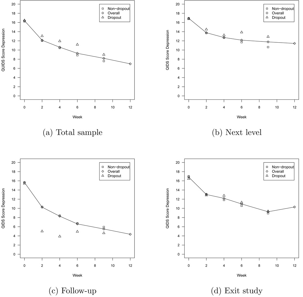
Figure 1 shows the mean curve over the six time points for the total sample and for subjects in each of the three Level 1 end-point categories. The figure also includes the average score among those who did and did not drop out at the next time point. It is seen that for the category Next level subjects with higher depression scores tend to drop out, whereas for the category Follow-up less depressed subjects tend to drop out.
Figure 1.
Sample means of the QIDS depression score at each visit
The missing at random (MAR; Little & Rubin, 2002) assumption of dropout as a function of the observed QIDS outcome is not necessarily fulfilled for subjects in any of the three Level 1 end-point categories. Variables not measured or not included in the model, that is, latent variables, may affect missingness. Some subjects may leave Level 1 because of not tolerating the medication, unrelated to the level of depression. Some subjects may leave the study for unknown reasons. Also, remission (moving subjects to follow-up) was typically determined by Hamilton-D, not the clinician-rated score used as the outcome in the analysis; Hamilton-D could not be used as the analysis outcome because it was measured only at baseline and end of Level 1. Modeling that explores possibly non-ignorable missing data is therefore of interest in order to draw proper inference to the population of subjects entering Level 1.
It should be emphasized that inference from the STAR*D study is limited by having no placebo group. There are no treatment groups to be compared during the Level 1 phase considered here. Muthén and Brown (2009) have shown how randomized designs with a placebo group enables causal effect estimation using growth mixture modeling, where placebo response can be taken into account. For studies with this design, the missing data modeling to be discussed here can be combined with the Muthén-Brown approach.
Pattern-mixture and selection modeling
Growth modeling analyses based on maximum-likelihood estimation typically use the assumption of missing at random (MAR; Little & Rubin, 2002). This covers situations where dropout is predicted by previously observed outcome values. Missing data due to dropout may not, however, fulfill the MAR assumption but may call for missing data techniques that handle non-ignorable missingness, sometimes referred to as not missing at random (NMAR). NMAR arises if unobserved variables that are correlated with the outcome predict missingness, such as a high or a low outcome value that is not recorded because the subject drops out. NMAR situation can be handled by using a “full-data” likelihood analysis which considers as data not only the outcomes but also 0/1 missing data indicators for each time point (see, e.g. Little, 2009). Consider the full-data likelihood in symbolic form where y refers to the outcome vector and m refers to the binary missing data indicators,
| (1) |
| (2) |
where the first expression refers to the the “pattern-mixture modeling” approach (see, e.g., Little, 1995) and the second expression to the “selection modeling” approach (see, e.g., Diggle & Kenward, 1994). “Shared-parameter modeling” considers the likelihood factorization
| (3) |
where c represents latent class variables influencing both the outcomes y and the missingness indicators m. Shared-parameter modeling may also use latent variables in the form of random effects, replacing the sum in (3) with integrals. It should be noted that each NMAR model involves untestable assumptions due to missing data. It is therefore important to compare results from several different models to achieve a sensitivity analysis. Recent overviews of NMAR modeling are given in Albert and Follman (2009) and Little (2009). In longitudinal studies, the non-ignorability concern is typically focused on missing data in the form of dropout, not intermittent missingness. This is the focus also of this study.
Pattern-mixture modeling
Pattern-mixture modeling (see, e.g., Little, 1995; Hedeker & Gibbons, 1997; Demirtas & Schafer, 2003) considers the likelihood factorization [y, d] = [y|d] [d], where the d variables can be represented by dummy variables for dropout occasion. A simple version of the model allows the random effect means to vary as a function of the dropout dummy variables. A quadratic growth model is used for STAR*D.
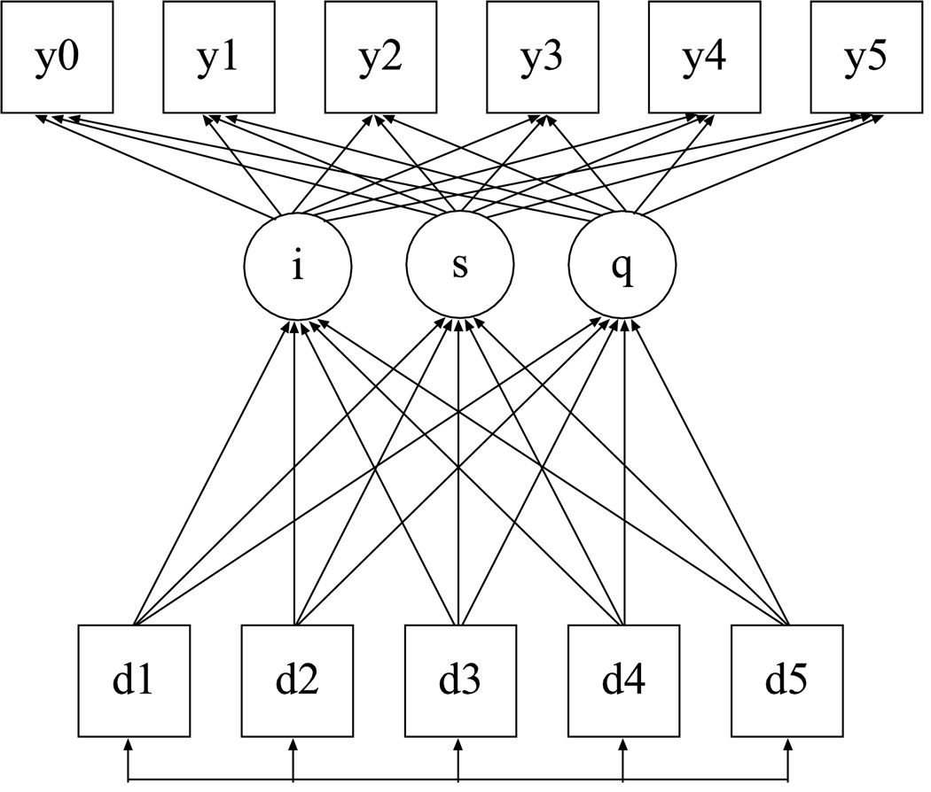
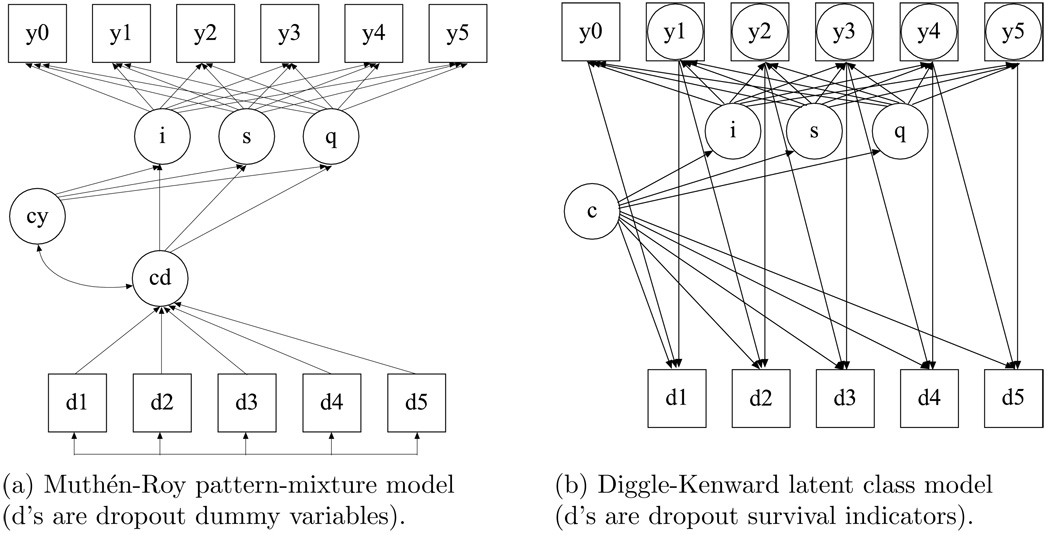
To facilitate understanding and comparisons of the alternative missing data models, the statistical description of the modeling is complemented by model diagrams. The pattern-mixture model is shown in model diagram form as in Figure 2, where squares represent observed variables and circles latent variables. Here, y0 – y5 represent the depression outcomes at baseline and through week 12, whereas i, s, and q represent the random intercept, slope, and quadratic slope. Note that these model diagrams are not geared towards causal inference. Single-headed arrows simply represent regression relationships and double-headed arrow represent correlations. The goal of the modeling is not to draw inference on causal effects, but to understand important sources of variation in the depression outcomes over time.
Figure 2.
Pattern-mixture modeling (d’s are dropout dummy variables)
The y0 – y5 outcomes show a total of 34 missing data patterns in the total sample of n = 4041. The dummy dropout indicators dt are defined as dt = 1 for a subject who drops out after time t − 1 (t = 1, 2, … 5) for the six time points. In the STAR*D data, the frequencies of dt = 1 are 420 (d1), 299 (d2), 301 (d3), 484 (d4), 983 (d5). There are 995 subjects who have all d’s equal to zero, that is, do not drop out. The five dummy dropout indicators thereby define six subgroups of subjects. Intermittent missingness is observed for 559 subjects. These subjects are spread among five of the six subgroups, excluding the d1 = 1 subgroup. Missing data is recorded for each subject and outcome variable. This implies that within each of the six subgroups, a subject with intermittent missingness is treated the same as a subject with complete data up to that point.
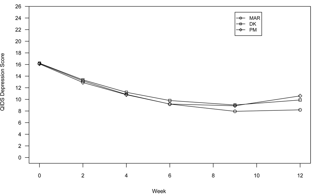
The pattern-mixture model typically needs restrictions on the parameters across dropout patterns. For example, with individuals dropping out after the first time point, the linear and quadratic slope means are not identified and for individuals dropping out after the second time point, the quadratic slope mean is not identified. In the current application of pattern-mixture modeling, these means are held equal to those of the pattern corresponding to dropping out one time point later. The random effect mean estimates are mixed over the patterns. This mixture can then be compared to the conventional single-class model estimated under MAR. The resulting estimated mean curve is shown in Figure 3. It is seen that the estimated mean QIDS depression score at week 12 is somewhat higher using pattern-mixture modeling than using MAR, as would be expected if dropouts have higher QIDS score. The week 12 QIDS standard deviation is 5.3 so that the difference is approximately half a standard deviation.
Figure 3.
Depression mean curves estimated under MAR, pattern-mixture (PM), and Diggle-Kenward selection modeling (DK)
Selection modeling
Selection modeling uses the likelihood factorization [y, d] = [y] [d|y], where the ds are survival indicators. An often cited model for selection modeling is the one proposed by Diggle and Kenward (1994). A common form of the Diggle-Kenward selection model assumes the logistic regression model for dropout,
| (4) |
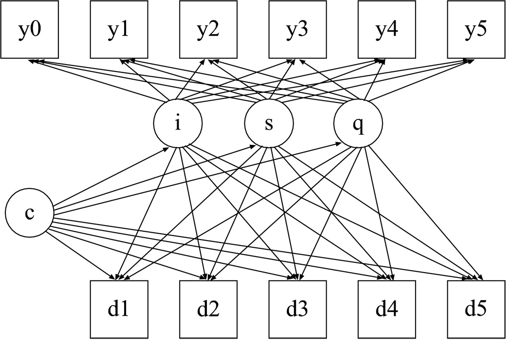
where the d variables are scored as discrete-time survival indicators, obtaining the value 0 for time periods before the dropout event occurs, 1 at the time period the dropout occurs, and missing for the time periods after the event occurs (Muthén & Masyn, 2005). Here, yti is missing for an individual who has dti = 1, that is, drops out after t − 1. According to this model, MAR holds if β1 = 0, that is, dropout is a function of the last observed y value, not the current latent y value.
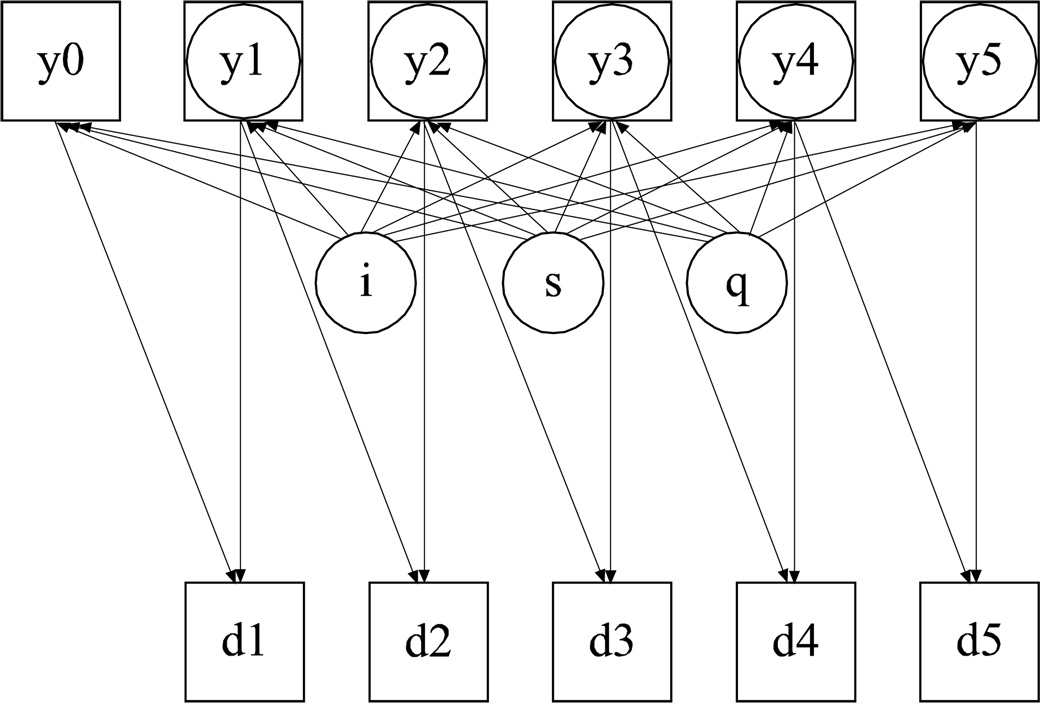
To complete the model, a quadratic growth curve is used as before for the STAR*D data. The model is shown in diagram form in Figure 4. Circles within squares represent variables that are not observed for the subjects who drop out.
Figure 4.
Diggle-Kenward selection modeling (d’s are survival indicators)
Applying the Diggle-Kenward model to the STAR*D data shows a significant positive maximum-likelihood (ML) estimate of β1. The significance of β1 suggests that NMAR modeling is of interest. The estimated mean depression curve for the Diggle-Kenward model is seen in Figure 3, showing a trajectory similar to the pattern-mixture model.
Model assumptions
It should be noted that MAR, pattern-mixture, and Diggle-Kenward selection modeling use different assumptions. It is instructive to consider the Diggle-Kenward model. If the model is correctly specified, β1 ≠ 0 in (4) may be viewed as an indication of NMAR. This, however, relies on the Diggle-Kenward model’s untestable assumptions about the selection process (4) and the normality assumptions which are made for unobserved variables. As stated by Little (1994) in the discussion of the article:
”Consider a single drop-out time, and let Y1 denote the (fully observed) variables up to drop-out and Y2 the (incompletely observed) variables after drop-out. The data clearly supply no direct information about the distribution of Y2 given Y1 for subjects who drop out. — differences in the distribution of Y2 given Y1 for those who do and do not drop out are solely determined by distributional assumptions of the model, such as the form of the model for drop-outs, normality, or constraints on the mean and covariance matrix.”
Considering ”the distribution of Y2 given Y1 for those who do and do not drop out” implies a conditioning on dropout, which means that the assumption of logistic regression for dropout is involved. Consequently, β1 ≠ 0 cannot be seen as a test rejecting MAR because assumptions not included in MAR are added in the Diggle-Kenward model.
MAR also makes normality assumptions for the outcomes which are untestable for the outcomes after dropout. But, the MAR assumptions do not involve a logistic regression for dropout. Pattern-mixture also makes normality assumptions for the outcomes, but the normality is conditional on dropout patterns. All in all, this implies that none of the models is a special case of the other. The models should all be applied and results compared.
MAR modeling with latent subgroups of subjects
In the context of the STAR*D depression example, the basic psychiatric hypothesis postulates a mixture of subjects who do and do not respond to the drug. In other words, there is a hypothesis of a latent class variable underlying the outcomes. This means that the conventional, single-class pattern-mixture and selection models are insufficient modeling tools for this example. Selection and shared-parameter modeling using a latent class variable has been suggested in the literature, but the emphasis has not been so much on recovering substantively-motivated trajectory classes as to represent non-ignorable missingness. Pattern-mixture modeling with a latent class variable has also been suggested in the literature, but merely to better summarize dropout patterns. In this section the MAR assumption is used and a description is given of growth mixture modeling with substantively-motivated trajectory classes. Later sections return to the study of growth mixtures in the context of pattern-mixture and selection modeling.
Of psychiatric concern in antidepressant trials such as STAR*D is to identify subjects who show either ”remission”, that is, have reached a sufficiently low depression level by the end of the trial, or ”response”, that is, have significantly dropped in depression level since baseline. The psychiatric definition of remission is in this case a Hamilton-D score ≤ 7 or a self-reported QIDS score ≤ 5. ”Response” is defined as a drop of at least 50% in the score from baseline. Such definitions are to some degree arbitrary and slightly different cutpoints can give quite different results. The approach may also suffer from large individual variability in the outcomes over time. Muthén et al. (2009) and Muthén and Brown (2009) used growth mixture modeling to instead define response as the percentage of subjects in a latent trajectory class with a distinctly low trajectory mean towards the end of the trial. This has the advantage of using information from all time points and focusing on trajectory shape. Growth mixture modeling combines random effects modeling in conventional repeated measures analysis with finite mixture modeling using latent class variables to represent qualitatively different classes of trajectories (Muthén & Shedden, 1999; Muthén et al., 2002; Muthén & Asparouhov, 2009). Growth mixture modeling is currently used in a wide variety of settings, see, e.g. Lin et al. (2002) for an application to the joint study of PSA development and prostate cancer survival, Elliott et al. (2005) for an application to identifying trajectories of positive affect and negative events following myocardial infarction, Beunckens et al. (2008) for an application to non-ignorable missing data modeling in a depression trial, and Muthén and Brown (2009) for an application to the estimation of drug effects in the presence of placebo response. Mixture modeling with missing data is also used in the context of models assuming latent ignorability as applied to non compliance in randomized trials; see, e.g. Frangakis and Rubin (1999), Muthén, Jo and Brown (2003), and Mealli et al. (2004).
Consider a quadratic growth mixture model with a latent trajectory class variable c assuming values k = 1, 2, …, K,
| (5) |
where the random effects distributions are allowed to vary as a function of the trajectory classes k,
| (6) |
| (7) |
| (8) |
The residuals ζi have zero means and a 3 × 3 covariance matrix Ψk, here taken to be constant across the latent classes. The residuals εti have zero means and a T × T covariance matrix Θk, here taken to be constant across classes as well. All residuals are assumed i.i.d and normally distributed. As an alternative, a 2-piece growth model can be used with a first linear piece describing early drug response during the first two weeks as in Uher et al. (2009) and Hunter et al. (2009). The 1-piece model is chosen here for simplicity and because the 2-piece model simply gives an elaboration with an additional minor class showing early response which at week 12 coincides with the low class of the 1-piece model. There was no evidence of a need for class-varying covariance matrices. As seen in Table 1 1–6 latent classes were studied. The conventional 1-class model is clearly superseded by multi-class models as judged by BIC. After 4 classes BIC decreases very little and the 5- and 6-class solutions offer only variations on the trajectory shapes found with 4 classes. The 4-class model is therefore considered here.
Table 1.
Summary of maximum-likelihood results for growth modeling assuming MAR and using a conventional 1-class model as well as a growth mixture model with 2–6 classes
| #classes | Loglikelihood | #par.s | BIC |
|---|---|---|---|
| 1 | −45137 | 15 | 90398 |
| 2 | −44961 | 19 | 90081 |
| 3 | −44922 | 23 | 90034 |
| 4 | −44890 | 27 | 90005 |
| 5 | −44873 | 31 | 90004 |
| 6 | −44852 | 35 | 89996 |
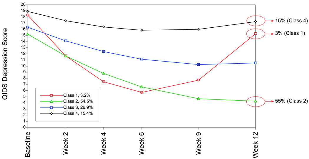
The 4-class GMM solution estimated under MAR is shown in Figure 5. The classes are well separated with a within-class standard deviation at week 12 of 2.42. From a substantive point of view, three of the four classes are of particular interest. It is seen that an estimated 55% of the subjects are in a distinct, low class (Class 2) showing drug response. An estimated 15% are in a high, non-responder class (Class 4). A minority class of 3% (Class 1) shows rapid initial improvement through week 6 with later worsening, a U-shaped curve that corresponds to transient improvement and possibly ”placebo only” response (Muthén & Brown, 2009). Placebo responders do not benefit from the drug but may benefit from the attention of the staff. The small size of the class, however, makes interpretation of this class questionable and it is of interest to see if NMAR modeling alternatives find this class.
Figure 5.
4-class growth mixture model estimated under MAR
The growth mixture modeling makes it clear that the single-class analyses using pattern-mixture and selection modeling shown in Figure 3 give a representation of the course of depression that is insufficient from a substantive point of view. The growth mixture modeling presented so far, however, assumes MAR and needs to be generalized to accommodate non-ignorable missingness as discussed in the sections to follow.
Existing NMAR models with latent subgroups of subjects
This section explores the STAR*D data using key NMAR models with latent subgroups of subjects suggested in the literature. First, a latent class version of the pattern-mixture model due to Roy (2003) is presented. Second, the Beunckens et al. (2008) mixture selection model is presented.
Roy latent dropout pattern-mixture modeling
The conventional pattern-mixture approach has been criticized in Roy (2003):
”One modeling approach is to assume the distribution … is a mixture over dropout patterns. However, this may lead to bias due to misclassification (i.e. by assuming every subject with the same dropout time has a common distribution). In addition, when there are a large number of unique patterns, this leads to sparse data. In that case, pattern-mixture models require further restrictions on the parameters for identifiability.”
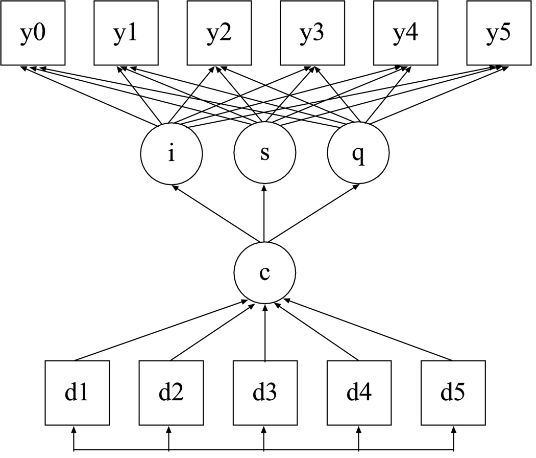
As an alternative to the conventional pattern-mixture model, Roy (2003) proposed a latent dropout pattern-mixture model using a latent class variable that is influenced by dropout time and influences the random effect means for the outcomes. Here, dropout time is a single covariate coded with discrete values. Instead of dropout time, Dantan et al. (2008) suggested using dummy variables for dropout occasion. Applied to the STAR*D data there is little difference in results using dropout time or dropout dummy variables. The Roy model implies a growth mixture model as in (5) – (8). Latent class membership is specified as a multinomial logistic regression using the dropout dummy variables as covariates,
| (9) |
This shows that the Roy latent dropout model can be seen as both a pattern-mixture type model and a “shared-parameter” model. Figure 6 shows the model diagram. Because of (9), the arrows from the dropout dummies point to the latent class variable and therefore indirectly to the outcomes.
Figure 6.
Roy latent class dropout modeling)
It should be emphasized that although the Roy model uses latent subgroups of subjects, the conceptualization of these subgroups is different from that of the growth mixture model in the previous section. Roy (2003) views the formation of latent subgroups as a better dropout classification of subjects than using observed dropout time. In contrast, growth mixture modeling views the latent subgroups as representing different outcome trajectory types, which may or may not be related to dropout time. As will be argued in a forthcoming section that presents a new type of Roy model, the latent subgroup formation in Roy (2003) is influenced not only by dropout time but also by trajectory type and this makes the interpretation of results from the Roy model less clear cut.
Table 2 shows the log likelihood, number of parameters, and BIC values for the conventional pattern-mixture model and the Roy latent dropout model for K = 2, 3, 4, 5. The superiority of the Roy model over the conventional pattern-mixture model is seen in the 2-class model having better log likelihood with fewer parameters. In terms of BIC, the 4-class model is preferable.
Table 2.
Summary of maximum-likelihood results for pattern-mixture modeling and Roy latent dropout modeling with 2–5 classes
| Model | Loglikelihood | #par.s | BIC |
|---|---|---|---|
| Pattern-mixture | −44946 | 27 | 90117 |
| Roy 2c | −44871 | 24 | 89942 |
| Roy 3c | −44777 | 33 | 89828 |
| Roy 4c | −44728 | 42 | 89806 |
| Roy 5c | −44698 | 51 | 89820 |
The ”misclassification” referred to in the above Roy (2003) quote is clearly evident in the STAR*D example. There is little agreement between the cross-classification of subjects using the six pattern-mixture dropout patterns versus using Roy 4-class latent dropout classes. As will be shown, this is likely due to the latent dropout classes being influenced also by trajectory types.
In line with conventional pattern-mixture modeling, the Roy latent dropout modeling is primarily focused on the mixture over the latent classes:
”While the class-specific estimates are informative, they are not of primary interest.” (Roy, 2003, p. 834)
The resulting depression mean curve estimated by Roy latent dropout modeling largely overlaps that of pattern-mixture modeling given in Figure 3 and is not shown. The curves of Figure 3, however, do not reveal if subgroups of subjects show different results under different NMAR models and under MAR.
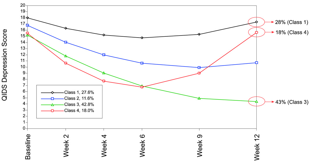
Instead of mixing over the four classes of the Roy latent dropout model, it is of interest to consider their interpretation in terms of antidepressant response and compare to the 4-class MAR growth mixture model of Figure 5. The four estimated mean depression curves are shown in Figure 7. The trajectory shapes and therefore the interpretations of the latent classes are in line with Figure 5. For the Roy model, only 43% of the subjects are estimated as responding with as many as 28% non responders and 18% showing a U-shaped curve of transient improvement. To conclude, the Roy NMAR model gives a considerably worse assessment of the drug efficiency than the 4-class MAR model.
Figure 7.
4-class Roy latent dropout model
Beunckens selection modeling with latent subgroups of subjects
Beunckens et al. (2008) introduced a model which combines selection modeling features with shared-parameter modeling features. The model has selection features in that it uses discrete-time survival dropout indicators as dependent variables influenced by the random effects of the outcome process for y in line with Wu and Carroll (1988). The model has shared-parameter modeling features in that both the survival dropout indicators and the depression outcomes are influenced by a latent class variable and random effects.
A special case of the model can be specified in line with Beunckens et al. (2008, equation 7), where the survival dropout indicators are influenced by both latent class as well as the random intercept η0i,
| (10) |
| (11) |
| (12) |
| (13) |
| (14) |
where in (14) the dependence of dropout on latent class in the first three terms is formulated as a quadratic latent class growth model which reduces the number of parameters relative to estimating free parameters for each class and time point. As before, the d variables are scored as discrete-time survival indicators, obtaining the value 0 for time periods before the dropout event occurs, 1 at the time period the dropout occurs, and missing for the time periods after the event occurs (Muthén & Masyn, 2005). The model is shown in diagram form in Figure 8.
Figure 8.
Beunckens mixture model (mixture Wu-Carroll model).
The results of fitting 1–5 classes are shown in Table 3. The 1-class model is in line with Wu and Carroll (1988). The 4-class model has the best BIC. For comparison the results for the Diggle-Kenward model are also given. It has a better BIC than the 1-class Beunckens model, but worse BIC than the 4-class Beunckens model.
Table 3.
Summary of maximum-likelihood results for Beunckens selection mixture modeling with 1–5 classes
| No. classes | Loglikelihood | #par.s | BIC |
|---|---|---|---|
| 1 | −51534 | 19 | 103225 |
| 2 | −51284 | 26 | 102784 |
| 3 | −51185 | 33 | 102644 |
| 4 | −51130 | 40 | 102592 |
| 5 | −51104 | 47 | 102597 |
| Diggle-Kenward | −51465 | 22 | 103113 |
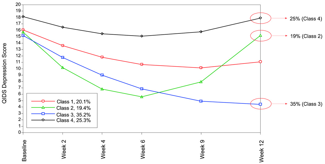
The estimated mean trajectories for the 4-class Beunckens model are shown in Figure 9. The low class of responding subjects is estimated as 35%, whereas the high class is estimated as 25% and the U-shaped class is estimated as 19%.
Figure 9.
4-class Beunckens selection mixture model
The Beunckens model is related to mixed-effects hybrid modeling (MEHM) proposed by Yuan and Little (2009). In both cases discrete-time survival is predicted by random effects (growth factors). While Beunckens lets the random effect means vary over latent classes, Yuan-Little lets the means vary over categories defined by dropout time. Because of the latent versus observed categories distinction, the Yuan-Little approach relates to the Beunckens approach much like pattern-mixture modeling relates to Roy modeling. The Yuan-Little modeling can be handled as in Figure 8, adding a covariate representing dropout time that influences the growth factors.
Extensions of NMAR models
This section explores the STAR*D data using two new NMAR models. First, the Roy pattern-mixture model is expanded, adding a second latent class variable. Next, the Diggle and Kenward selection model is generalized to include latent subgroups of subjects.
Pattern-mixture modeling: Muthén-Roy modeling with latent subgroups of subjects
For both conventional pattern-mixture modeling and Roy latent dropout modeling the intention is to mix the parameter estimates over the patterns/classes to obtain an overall estimated growth curve. This mixing may, however, hide substantively interesting trajectory classes. Furthermore, the Roy approach forms classes based not only on the relationship between dropout and outcomes, but also based on the development of the outcomes over time. This may confound dropout classes with trajectory classes.
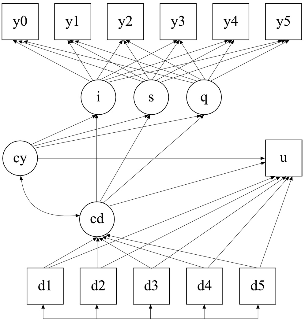
To alleviate these concerns, a new type of pattern-mixture model is introduced here, using a generalization that allows for two distinct latent class variables: one related to dropout and another related to the outcome trajectories. The former latent class variable summarizes dropout patterns and the latter provides information about substantively interesting trajectory classes. The model will be referred to as the Muthén-Roy model and is specified as follows, defining a latent class variable cd for K dropout groups and a latent class variable cy for L trajectory types of the depression outcome y.
| (15) |
| (16) |
| (17) |
| (18) |
The two latent class membership relationships
| (19) |
| (20) |
can be combined in the following bivariate loglinear form where cd and cy are allowed to correlate via γ0ydkl,
| (21) |
where γ0dk, γ0yl, γ0ydkl, γtk are fixed to 0 for identification purposes when either k or l are the last class categories. Part (a) of Figure 10 shows the model in diagram form.
Figure 10.
NMAR modeling extensions.
It is clear from (19) and (20) that cd and cy play different roles in the model. While both cd and cy influence the random effects, cy is not influenced by the dropout dummy variables. One way to view the model is that cy represents substantively different trajectory shapes which are moderated by cd within each cy class. Centering at the first time point so that the random intercept η0 is the systematic part of the variation in the baseline y outcome, this way of viewing the model is emphasized by holding the random intercept means for each cy class equal across the cd classes.
Table 4 gives the results for a series of Muthén-Roy models. The table shows that the 3cy, 2cd Muthén-Roy model uses fewer parameters than the Roy 4c model (also referred to as 1cy, 4cd), but has a better log likelihood value. The best BIC is obtained for the 4cy, 2cd Muthén-Roy model. With two dropout classes, the classes are distinguished only by a stronger or weaker tendency to drop out, with no differentiation of the timing of dropout. A class with a higher dropout tendency can, however, exhibit different curve shapes in combination with different trajectory classes as will be seen next.
Table 4.
Comparing maximum-likelihood results for Roy and Muthén-Roy mixture models
| Model | Loglikelihood | # par.’s | BIC |
|---|---|---|---|
| Roy 4c (1cy, 4cd) | −44728 | 42 | 89806 |
| Muthén-Roy 2cy, 2cd | −44743 | 30 | 89736 |
| Muthén-Roy 2cy, 3cd | −44702 | 41 | 89744 |
| Muthén-Roy 2cy, 4cd | −44654 | 52 | 89740 |
| Muthén-Roy 3cy, 2cd | −44696 | 37 | 89699 |
| Muthén-Roy 3cy, 3cd | −44647 | 51 | 89717 |
| Muthén-Roy 4cy, 2cd | −44662 | 44 | 89689 |
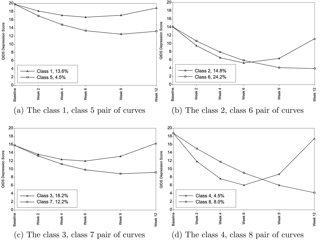
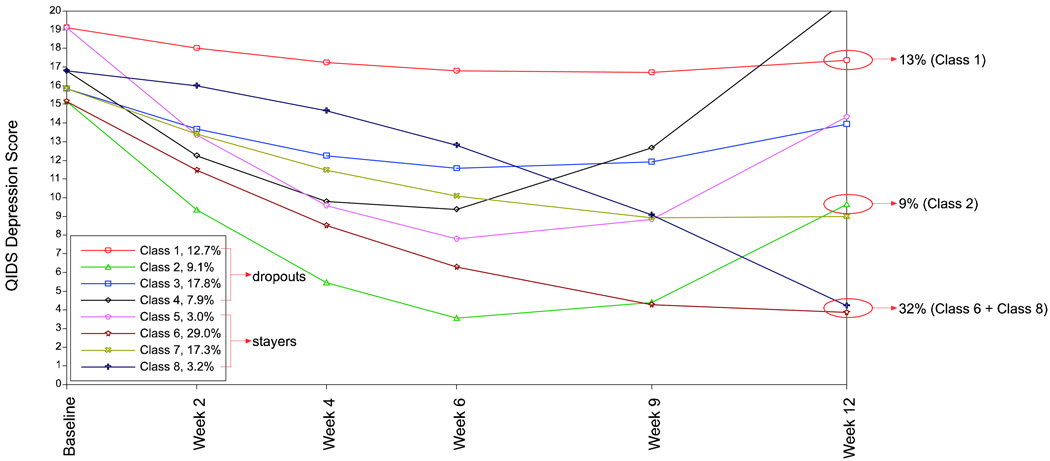
The estimated mean curves for the 4cy, 2cd Muthén-Roy model are shown in Figure 11. The model uses eight classes, combining the four cy classes and the two cd classes. To simplify the figure visually, the eight curves are separated into four panels. Because of the random intercept mean equalities, giving the same baseline value, there are four pairs of curves. The estimates for the γ slope parameters of the logistic regression (19) show that subjects who drop out are more likely to be in cd class 1. The curves corresponding to the dropout class (cd = 1) are marked with triangles. Classes 1 – 4 are classes where subjects have a higher tendency to drop out and classes 5–8 are classes where subjects have a higher tendency to stay in the study. The legends give the class percentages for the different curves.
Figure 11.
Muthén-Roy mixture model with 4 trajectory classes and 2 dropout classes (curves marked with triangles correspond to a higher tendency to drop out)
It is interesting to compare the estimated dropout curves of Figure 11 to the Figure 1 observed means before dropout denoted by triangles. The Figure 11 dropout curves for panel (a) and panel (c) appear to reflect the observed means for subjects moved to the next level seen in Figure 1, panel (b). The Figure 11 U-shaped dropout curves for panel (b) and panel (d) appear to reflect the observed means for subjects moved to follow-up seen in Figure 1, panel (c). These relationships are explored in a later section.
Panel (b) shows two classes with similar development of decreasing depression scores up to week 6, where both curves are close to the level deemed as ”remittance”. The 14.8% class 2 subjects, however, show a U-shaped curve with a substantially worsening depression level by week 12 whereas the 24% class 6 subjects respond. It is of substantive interest to further explore the different characteristics of subjects in these two classes. Class 2 subjects may be prematurely moved to the follow-up phase.
A second U-shaped curve is found in class 4 with 4.5% of the subjects, although not dipping as low as for class 2. A second class, class 8 with 8%, shows response adding to a total 32% showing response using this model. The corresponding percentage for the U-shaped class of the 4-class Roy model is similar at 18%, while the response class percentage of 43% is somewhat higher. Choosing between models is discussed in a later section.
Selection modeling: Diggle-Kenward modeling with latent subgroups of subjects
The Diggle-Kenward model may be contrasted with the Beunckens model. In the former, the survival dropout indicators are influenced directly by the depression outcomes. In the 1-class case, this gives a better BIC than having survival be influenced by random effects. The use of multiple classes, however, makes the Beunckens model have a better BIC than Diggle-Kenward. For these reasons, the Diggle-Kenward model is here extended to a mixture model specified as follows.
| (22) |
| (23) |
| (24) |
| (25) |
| (26) |
Alternatively, a quadratic latent class growth model can be specified for the αtk coefficients in line with (14). The logistic regression slopes β of (26) are here allowed to vary across the latent classes. This is important because subjects in high trajectory classes tend to drop out due to high depression values, while subjects in the low class tend to drop out due to low depression values.
To provide further generality the β slopes are allowed to also vary across time. For example, a subject’s dropout probability may be less influenced by the depression score early in the study while later failure to reduce depression may have greater influence on dropout. The model is shown in diagram form in part (b) of Figure 10.
Table 5 shows the results of fitting a series of Diggle-Kenward selection mixture models using four classes as for the Beunckens model. For comparison, the conventional 1-class Diggle-Kenward model is also presented. The 4-class model 1 specifies class- and time-invariant β slopes in (26) as well as class-invariant αt values. The 4-class model 2 allows class-varying β and class-varying αt, where the class variation in α is specified as a quadratic function as in (14). The 4-class model 3 is as the 4-class model 2 but also allows β variation across time. It is clear from both BIC and likelihood-ratio χ2 testing that the 4-class model 3 is preferable. Based on BIC, this model is also preferable to the 4-class Beunckens model of Table 3.
Table 5.
Summary of maximum-likelihood results for Diggle-Kenward selection mixture modeling
| Model | Loglikelihood | #par.s | BIC |
|---|---|---|---|
| 4-class model 1 | −51159 | 34 | 102600 |
| 4-class model 2 | −50983 | 47 | 102356 |
| 4-class model 3 | −50670 | 76 | 101971 |
| 1-class model | −51465 | 22 | 103113 |
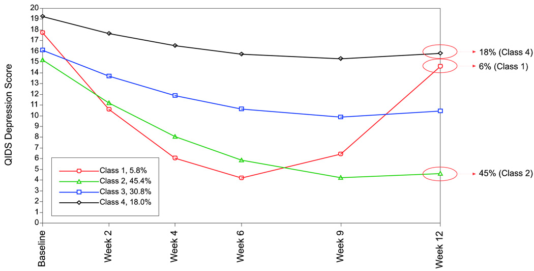
The estimated mean curves for the 4-class model 3 are shown in Figure 12. The low class of subjects who respond is estimated as 45%, the high class of non responders is estimated as 18%, whereas the U-shaped class is estimated as 6%. These estimates lie in between of those obtained with MAR on the one hand and Muthén-Roy and Beunckens on the other hand.
Figure 12.
4-class Diggle-Kenward selection mixture model
Comparing models
Summary of percentages
This section summarizes the results for the preferred models: the 4-class model in the MAR family, the Muthén-Roy 4c, 2c model in the pattern-mixture family, and the Diggle-Kenward 4-class model 3 in the selection family. Table 6 gives the model-estimated percentages for the high class, the U-shaped class, and the low class for these three models.
Table 6.
Summary of key model-estimated percentages for latent class, remission, and response
| Model | High Class |
U-shaped Class |
Low Class |
Remission (≤ 5) |
Response (≥ 50% drop) |
|---|---|---|---|---|---|
| MAR 4c | 15 | 3 | 55 | 34 | 53 |
| Muthén-Roy 4c, 2c | 14 | 15 | 32 | 22 | 34 |
| Diggle-Kenward 4c | 18 | 6 | 45 | 26 | 45 |
| MAR 1c | 27 | 49 | |||
It is also useful to consider model-estimated results presented in the traditional form of antidepressant trials. Traditionally, remission is defined as an endpoint depression score less than a certain cutpoint, in this case week 12 QIDS score ≤ 5. Also, drug response is defined as a drop in the depression score of at least 50% from baseline to week 12. Table 6 also includes these percentages for the three models, as well as for the traditional 1-class MAR model.
It is clear from Table 6 that the models have a wide range of estimates for the percentage in the three latent classes. The 4-class MAR model has a high response rate of 55% with a total of only 18% in the failing high and U-shaped classes. This gives a much more positive view of the antidepressant than the Muthén-Roy model’s 32% responders and 29% in the failing high and U-shaped classes.
For all the models, the low class percentage is closer to the response percentage than the remission percentage. Although the mean of the low class at week 12 is below the ≤ 5 cutoff, not all subjects in the class are. Instead, the trajectory shape determines the class membership.
Choosing between models
Choosing between the MAR, pattern-mixture, and selection models is difficult given that the three model types have different likelihood and BIC metrics. The different metrics are due to the models having different sets of dependent variables. The loglikelihoods of pattern-mixture, Roy, and Muthén-Roy models are comparable. Likewise, the selection models of Diggle-Kenward and Beunckens have comparable loglikelihoods. Comparing loglikelihoods between models not belonging to the same family, however, is not informative. Nor are the loglikelihoods for either NMAR family comparable to MAR models, a fact that is not always made clear in the NMAR literature. For example, it is not correct to view the MAR mixture model as a special case of the Roy model where there is no influence of dropout indicators on latent class membership, that is, γtk = 0 in (9). This is because the MAR model allows for dropout and the y outcome to be related in that observed y values are allowed to influence dropout (see, e.g., Demirtas & Schafer, 2003).
The question arises which analysis strategy a researcher should take with dropout. It is suggested here that a first step is to find the best model using BIC within each of the three families of models, MAR (including both single- and multiple-class models), pattern-mixture (including Roy and Muthén-Roy modeling), and selection (single- and multiple-class models). If results from the three approaches all agree, then the MAR results are supported and a researcher can present the MAR results with the additional information that NMAR explorations do not contradict the findings. If pattern-mixture and selection modeling agree, but the MAR results disagree in substantively important ways, it seems reasonable to present both the MAR and NMAR results and raise the possibility that the NMAR results may be more trustworthy. If results from all three approaches disagree, there is no statistical basis for preferring the results any of the models. Instead, the range of results need to be reported as in Table 6.
In some exceptional cases, however, the models can be compared in terms of how they relate to auxiliary information about the reasons for dropout. Such information is fortunately available in the STAR*D data. This is explored next.
Adding auxiliary information
The STAR*D data have useful auxiliary information in the form of the subject’s ending status in the 12-week Level 1 part of the trial. As mentioned in the introduction, STAR*D distinguished between three different end categories: Subjects were moved to the next level if the medication was not completely effective or not tolerated; subjects were moved to follow-up if showing remission; or subjects exited the study for unknown reasons. Adding a missing data category, this gives a four-category nominal variable u, say, standing for ultimate, or distal, outcome. The three competing models, MAR, Muthén-Roy, and mixture Diggle-Kenward, can be augmented by the u outcome, where the added parameters are the three u probabilities varying across the latent classes of those models. The u variable is useful for NMAR modeling because it carries more information than the observed y outcome given that it also relates to side effects and subject preferences. The ability of the original model to capture non-ignorable missingness can be assessed by studying the congruence between the latent class formation when not including versus including the u variable in the model.
The Muthén-Roy model can be extended to allow u to be influenced not only by the two latent class variables cd and cy, but also the dropout indicators d. For r = 1, 2, …, R (R = 4),
| (27) |
Figure 13 shows the extended Muthén-Roy model in diagram form. In the extended model, the relationship between latent class membership and the end categories provides a predictive validity check of the latent classes.
Figure 13.
Muthén-Roy model extended to include an ultimate outcome
Figure 14 shows the estimated mean curves for the MAR and mixture Diggle-Kenward models extended to include u. Figure 15 shows the estimated mean curves for the extended Muthén-Roy model. Unlike for Figure 11 the eight curves are shown in a single graph. The specification in (27) was used for Muthén-Roy, where including the d’s as covariates influencing u improved the BIC but had little effect on the parameter estimates.
Figure 14.
(a) Estimated means under the MAR model extended to include an ultimate outcome. (b) Estimated means under the mixture Diggle-Kenward model extended to include an ultimate outcome.
Figure 15.
Estimated means under the Muthén-Roy model extended to include an ultimate outcome
The extended MAR model retains the trajectory shapes of the original latent classes, but it is seen that it obtains a lower percentage in the low class than in the original MAR model, 42% compared to 55%. The extended mixture Diggle-Kenward model also obtains a reduced percentage in the low class, 37% as compared to 45%. The high class is reduced from 18% to 15%. The extended mixture Diggle-Kenward model does not, however, retain the U-shaped class of the original Diggle-Kenward model. The extended Muthén-Roy model largely retains the trajectory shapes of the original model. The low class percentage remains unchanged at 32% and the high class percentage changes only from 14% to 13%. The U-shaped class is now more clearly accentuated and distinguished as the only class that shows a substantial temporary improvement, with an outcome well below 5, and subsequent worsening. The class percentage is changed from 15% to 9%. All in all, the Muthén-Roy model appears as the model most congruent with the u outcome.
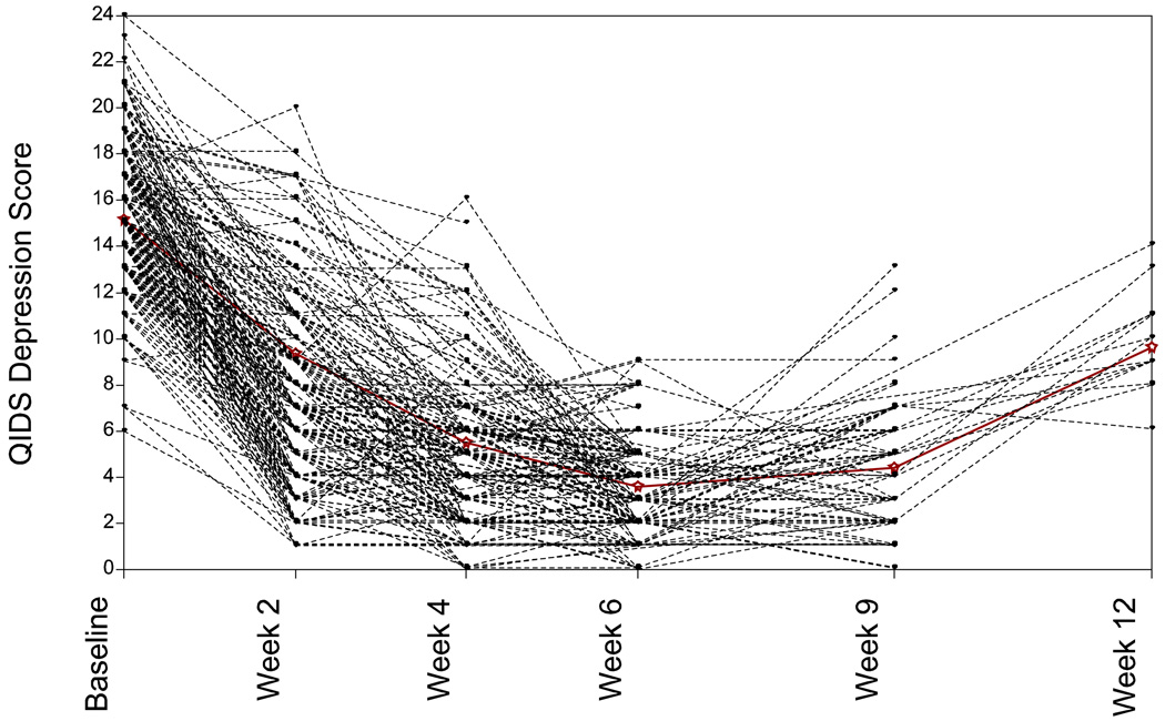
The Muthén-Roy plot shows an interesting phenomenon related to the U-shaped class and the low class. Starting out the same as the low class, the U-shaped class has the higher dropout tendency. This is because many subjects in the 9% U-shaped class have a score ≤ 5 and are likely to be moved to follow-up. The U-shaped class, however, is characterized by a temporary improvement and later worsening. The low class estimate of 37% in the extended mixture Diggle-Kenward model may be biased upwards because it does not allow for a portion of those subjects following U-shaped trajectories. The existence of such subjects in the data is demonstrated in Figure 16 showing observed trajectories for subjects classified into the U-shaped class by the extended Muthén-Roy model. In this sense, the Muthén-Roy model appears more flexible than the mixture Diggle-Kenward model in this application.
Figure 16.
Observed individual trajectories for subjects classified into the U-shaped class using the extended Muthén-Roy model
Table 7 considers the predictive aspects of the latent classes. It shows the estimated probabilities for the four categories of the ultimate outcome u given latent class membership for the extended Muthén-Roy model. Subjects in the low class have a high probability of ending up in the follow-up category corresponding to remission. Subjects in the high class are likely to be moved to the next level with treatment by other antidepressants, but have a sizable probability of exiting the study. Subjects in the U-shaped class are likely to be moved to follow-up but also have a sizable probability of exiting the study. The high percentage (62%) moved to follow-up in this class of rapid but transient improvement points to a problem of counting these individuals as remitters.
Table 7.
Estimated probabilities for the ultimate outcome given latent class membership for the extended Muthén-Roy model
| Latent class | Next level | Follow-up | Exit | Missing |
|---|---|---|---|---|
| Low | 0.00 | 0.94 | 0.04 | 0.02 |
| High | 0.63 | 0.00 | 0.37 | 0.00 |
| U | 0.09 | 0.62 | 0.29 | 0.00 |
Conclusions
It is of interest to see if the growth mixture model results under MAR are trustworthy given that missingness may be NMAR. Applying a series of NMAR models in a sensitivity analysis provides useful information regarding this question. On the whole, the MAR mixture model results, the Muthén-Roy mixture model results, and the mixture Diggle-Kenward selection model results for the STAR*D data have similarities in terms of trajectory shapes. The models do differ, however, in the latent trajectory class percentages, which impacts the assessment of the drug effectiveness. The conventional MAR 4-class model estimates that 55% of the subjects are in the response class with 18% in failing classes, whereas the extended Muthén-Roy model gives the response estimate 32% with 29% in failing classes. Follow-up analysis using the Level 1 ultimate outcome classification in the STAR*D trial lends credence to the Muthén-Roy estimate. Furthermore, the Muthén-Roy finding of a 9% U-shaped class of subjects who may be prematurely deemed as remitting is of clinical importance in that it suggests a transient improvement.
The different models have quite different computational demands in the maximum-likelihood estimation. The MAR mixture model has rather light computations, the Muthén-Roy model has moderately heavy computations, and the mixture Diggle-Kenward model has very heavy computations. The EM computations of the mixture Diggle-Kenward model involve numerical integration over the unobserved outcomes which is handled via Monte Carlo integration. Combined with using many random starting values to avoid local maxima, this leads to quite slow computations. The Beunckens’ model is lighter in this regard, given that integration needs to be done only with respect to the random effects. Scripts for the analyses are available at http://www.statmodel.com/examples/penn.shtml#stard using the Mplus program (Muthén & Muthén, 1998–2009).
The modeling can also be extended in several ways within the general latent variable framework handled in Mplus. Covariates can predict the latent class variables as well as random effects within class and outcomes directly. Outcomes can be binary, ordered polytomous, censored-normal, and counts. Multilevel data can be handled with level 2 latent class variables.
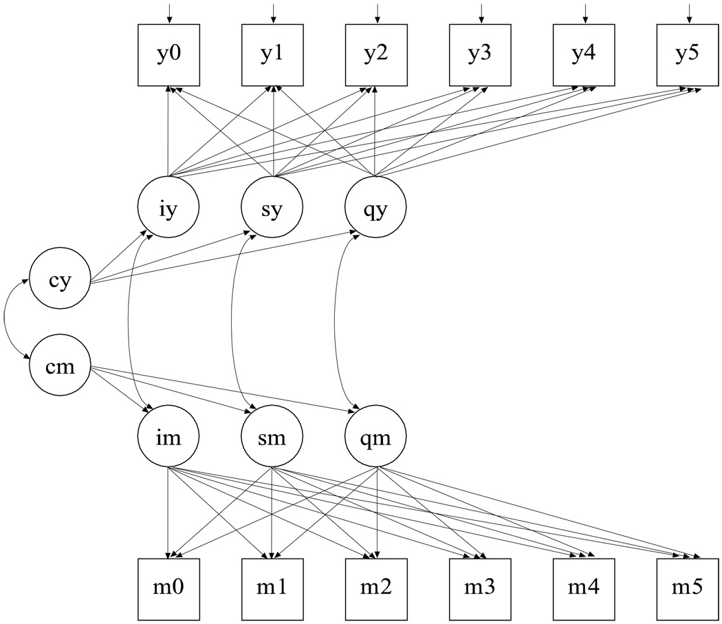
In addition to modeling dropout, the general latent variable framework can also handle modeling of the binary missing data indicators m so that intermittent missingness is included. For example, it is possible to apply a two-part (semi-continuous) growth mixture model extending the work of Olsen and Schafer (2001). The model can be expressed as two parallel processes, one for the outcomes and one for the binary missing data indicators. At a given time point, the outcome is missing or not depending on the missing data indicator. The two processes have growth models with latent class variables and random effects that are correlated across the processes. Such a model is shown in diagram form in Figure 17.
Figure 17.
2-part model for joint growth mixture modeling of missing data indicators and outcomes
In the current STAR*D example, a large sample size is available for analysis (n = 4041). Many data sets in psychology are of considerably smaller size. Fortunately, a large sample size is not a prerequisite for NMAR analysis. For example, the schizophrenia example in Demirtas and Schafer (2003) using n = 437 was successfully reanalyzed with 2-class pattern-mixture and selection models. It is likely that smaller samples can also be used as long as the trajectory classes are sufficiently well separated. To determine the performance of the analyses, simulation studies can be carried out in Mplus, where different types of NMAR missing data can be generated.
Acknowledgments
The third author was supported by NIMH grant No. 1R34MH085933-01 (P.I., AM Hunter). The authors thank Hendricks Brown, Rudolf Uher, and Tom Belin for helpful comments on an earlier version. The assistance of Shaunna Clark and Jackie Ho is gratefully acknowledged.
For further correspondence, please contact Bengt Muthén at 3463 Stoner Ave, Los Angeles, CA. 90066.
References
- Albert PS, Follman DA. Shared-parameter models. In: Fitzmaurice G, Davidian M, Verbeke G, Molenberghs G, editors. Longitudinal Data Analysis. Boca Raton: Chapman & Hall/CRC Press; 2009. pp. 433–452. [Google Scholar]
- Beunckens C, Molenberghs G, Verbeke G, Mallinckrodt C. A latent-class mixture model for incomplete longitudinal Gaussian data. Biometrics. 2008;64:96–105. doi: 10.1111/j.1541-0420.2007.00837.x. [DOI] [PubMed] [Google Scholar]
- Dantan E, Proust-Lima C, Letenneur L, Jacqmin-Gadda H. Pattern mixture models and latent class models for the analysis of multivariate longitudinal data with informative dropouts. The International Journal of Biostatistics. 2008;4:1–26. doi: 10.2202/1557-4679.1088. [DOI] [PubMed] [Google Scholar]
- Demirtas H, Schafer JL. On the performance of random-coefficient pattern-mixture models for non-ignorable drop-out. Statistics in Medicine. 2003;22:2553–2575. doi: 10.1002/sim.1475. [DOI] [PubMed] [Google Scholar]
- Diggle PD, Kenward MG. Informative dropout in longitudinal data analysis (with discussion) Applied Statistics. 1994;43:49–73. [Google Scholar]
- Elliott MR, Gallo JJ, Ten Have TR, Bogner HR, Katz IR. Using a Bayesian latent growth curve model to identify trajectories of positive affect and negative events following myocardial infarction. Biostatistics. 2005;6:119–143. doi: 10.1093/biostatistics/kxh022. [DOI] [PMC free article] [PubMed] [Google Scholar]
- Frangakis CE, Rubin DB. Addressing complications of intention-to-treat analysis in the presence of all-or-none treatment-noncompliance and subsequent missing outcomes. Biometrika. 1999;86:365379. [Google Scholar]
- Hedeker D, Gibbons RD. Application of random-effects pattern-mixture models for missing data in longitudinal studies. Psychological Methods. 1997;2:64–78. [Google Scholar]
- Hunter AM, Muthén BO, Cook IA, Leuchter AF. Antidepressant response trajectories and quantitative electroencephalography (QEEG) biomarkers in major depressive disorder. Journal of Psychiatric Research. 2009;44:90–98. doi: 10.1016/j.jpsychires.2009.06.006. [DOI] [PMC free article] [PubMed] [Google Scholar]
- Lin H, Turnbull BW, McCulloch CE, Slate E. Latent class models for joint analysis of longitudinal biomarker and event process data: application to longitudinal prostate-specific antigen readings and prostate cancer. Journal of the American Statistical Association. 2002;97:53–65. [Google Scholar]
- Lin H, McCullogh CE, Rosenheck RA. Latent pattern mixture models for informative intermittent missing data in longitudinal studies. Biometrics. 2004;60:295–305. doi: 10.1111/j.0006-341X.2004.00173.x. [DOI] [PubMed] [Google Scholar]
- Little RJ. Discussion of the paper by Diggle and Kenward. Applied Statistics. 1994;43:86. [Google Scholar]
- Little RJ. Modeling the drop-out mechanism in repeated-measures studies. Journal of the American Statistical Association. 1995;90:1112–1121. [Google Scholar]
- Little RJ. Selection and pattern-mixture models. In: Fitzmaurice G, Davidian M, Verbeke G, Molenberghs G, editors. Longitudinal Data Analysis. Boca Raton: Chapman & Hall/CRC Press; 2009. pp. 409–431. [Google Scholar]
- Little RJ, Rubin DB. Statistical analysis with missing data. Second edition. New York: John Wiley and Sons; 2002. [Google Scholar]
- McLachlan GJ, Peel D. Finite mixture models. New York: Wiley and Sons; 2000. [Google Scholar]
- Mealli F, Imbens GW, Ferro S, Biggeri A. Analyzing a randomized trial on breast self-examination with noncompliance and missing outcomes. Biostatistics. 2004;5:207–222. doi: 10.1093/biostatistics/5.2.207. [DOI] [PubMed] [Google Scholar]
- Muthén B, Asparouhov T. Growth mixture modeling: Analysis with non-Gaussian random effects. In: Fitzmaurice G, Davidian M, Verbeke G, Molenberghs G, editors. Longitudinal Data Analysis. Boca Raton: Chapman & Hall/CRC Press; 2009. pp. 143–165. [Google Scholar]
- Muthén B, Brown H, Leuchter A, Hunter A. Forthcoming in P.E. Shrout (ed.), Causality and Psychopathology: Finding the Determinants of Disorders and their Cures. Washington, DC: American Psychiatric Publishing; 2009. General approaches to analysis of course: Applying growth mixture modeling to randomized trials of depression medication. [Google Scholar]
- Muthén B, Brown CH. Estimating drug effects in the presence of placebo response: Causal inference using growth mixture modeling. Statistics in Medicine. 2009;28:3363–3385. doi: 10.1002/sim.3721. [DOI] [PMC free article] [PubMed] [Google Scholar]
- Muthén B, Brown CH, Masyn K, Jo B, Khoo ST, Yang CC, Wang CP, Kellam S, Carlin J, Liao J. General growth mixture modeling for randomized preventive interventions. Biostatistics. 2002;3:459–475. doi: 10.1093/biostatistics/3.4.459. [DOI] [PubMed] [Google Scholar]
- Muthén B, Jo B, Brown H. Comment on the Barnard, Frangakis, Hill & Rubin article, Principal stratification approach to broken randomized experiments: A case study of school choice vouchers in New York City. Journal of the American Statistical Association. 2003;98:311–314. [Google Scholar]
- Muthén B, Masyn K. Discrete-time survival mixture analysis. Journal of Educational and Behavioral Statistics. 2005;30:27–58. [Google Scholar]
- Muthén B, Muthén L. Mplus User’s Guide. Sixth Edition. Los Angeles, CA: Muthén & Muthén; 1998–20010. [Google Scholar]
- Muthén B, Shedden K. Finite mixture modeling with mixture outcomes using the EM algorithm. Biometrics. 1999;55:463–469. doi: 10.1111/j.0006-341x.1999.00463.x. [DOI] [PubMed] [Google Scholar]
- Olsen MK, Schafer JL. A two-part random effects model for semicontinuous longitudinal data. Journal of the American Statistical Association. 2001;96:730–745. [Google Scholar]
- Roy J. Modeling longitudinal data with nonignorable dropouts using a latent dropout class model. Biometrics. 2003;59:829–836. doi: 10.1111/j.0006-341x.2003.00097.x. [DOI] [PubMed] [Google Scholar]
- Roy J, Daniels MJ. A general class of pattern mixture models for nonignorable dropout with many possible dropout times. Biometrics. 2008;64:538–545. doi: 10.1111/j.1541-0420.2007.00884.x. [DOI] [PMC free article] [PubMed] [Google Scholar]
- Rush AJ, Fava M, Wisniewski SR, et al. Controlled Clinical Trials. 2004;25:119–142. doi: 10.1016/s0197-2456(03)00112-0. [DOI] [PubMed] [Google Scholar]
- Trivedi MH, Rush AJ, Wisniewski SR, et al. Evaluation of outcomes with citalopram for depression using measurement-based care in STAR*D: implications for clinical practice. The American Journal of Psychiatry. 2006;163(1):28–40. doi: 10.1176/appi.ajp.163.1.28. [DOI] [PubMed] [Google Scholar]
- Uher R, Muthén B, Souery D, Mors O, Jaracz J, Placentino A, Petrovic A, Zobel A, Henigsberg N, Rietschel M, Aitchison K, Farmer A, McGuffin P. Trajectories of change in depression severity during treatment with antidepressants. Psychological Medicine. 2009 doi: 10.1017/S0033291709991528. published online October 29, 2009. [DOI] [PubMed] [Google Scholar]
- Wu MC, Carroll RJ. Estimation and comparison of changes in the presence of informative right censoring by modeling the censoring process. Biometrics. 1988;44:175–188. [Google Scholar]
- Yuan Y, Little RJA. Mixed-effect hybrid models for longitudinal data with nonignorable dropout. Biometrics. 2009;65:478–486. doi: 10.1111/j.1541-0420.2008.01102.x. [DOI] [PubMed] [Google Scholar]


