Prediction of feather damage in laying hens using optical flows and Markov models

Abstract

Feather pecking in laying hens is a major welfare and production problem for commercial egg producers, resulting in mortality, loss of production as well as welfare issues for the damaged birds. Damaging outbreaks of feather pecking are currently impossible to control, despite a number of proposed interventions. However, the ability to predict feather damage in advance would be a valuable research tool for identifying which management or environmental factors could be the most effective interventions at different ages. This paper proposes a framework for forecasting the damage caused by injurious pecking based on automated image processing and statistical analysis. By frame-by-frame analysis of video recordings of laying hen flocks, optical flow measures are calculated as indicators of the movement of the birds. From the optical flow datasets, measures of disturbance are extracted using hidden Markov models. Based on these disturbance measures and age-related variables, the levels of feather damage in flocks in future weeks is predicted. Applying the proposed method to real-world datasets, it is shown that the disturbance measures offer improved predictive values for feather damage thus enabling an identification of flocks with probable prevalence of damage and injury later in lay.

1. Introduction

A major welfare problem in commercial egg production is that of injurious feather pecking, where the hens peck each other's feathers and skin, leading to feather damage, injury and even cannibalism [1,2]. The problem is worse in barn and free-range systems than in cages [3,4] and so is likely to become even more widespread with the European Union ban on barren cages in 2012. Feather pecking increases feed consumption owing to heat loss [5], reduces egg production [6], causes pain and suffering of the injured birds [7] and increases bird mortality, including cannibalism [8]. Despite a great deal of research it is currently not possible to prevent feather pecking altogether [1,2]. The main method of controlling it is to blunt the birds' beaks to reduce the damage they can do to each other. This blunting is usually done when they are day-olds by use of hot-blade or infra-red beak treatment [9], but it raises welfare problems in its own right [10]. A major research priority is therefore to eliminate feather pecking without resorting to beak trimming.

An important step forward would be an ability to predict outbreaks of feather pecking in advance and to identify those flocks that were at particular risk of damage [11]. A large number of interventions such as changing the litter, changing the lighting, changing the methods of providing food and water, changing the times of feeding have been proposed, although none are currently completely effective [1,2]. Some of these would cause considerable expense and so it is important to know those or which combinations are most effective and to target the most at-risk flocks. Being able to analyse the effects of such interventions, or other management practices, at an early stage will help to identify key factors in this problem.

This paper proposes a novel method for predicting feather damage based on visual processing and statistical analysis of flock behaviour taken from video recordings. We show that a disturbance profile can be generated for a flock based on optical flow measures of the movements of the birds [12] and the use of hidden Markov models (HMMs; [13]). We then show that this disturbance profile, together with other measures such as the age of the birds, has predictive power as to which flocks will develop severe feather damage in the future.

2. Data collection

The procedure is outlined in figure 1. We used video recordings taken inside commercial free-range laying houses for our basic data.

Figure 1.

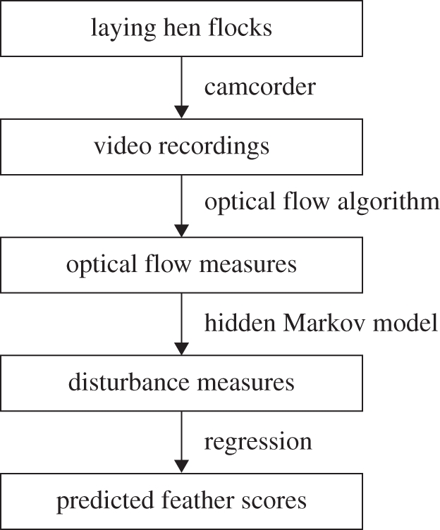
Outline of the method.

2.1. Video recordings and laying flocks

The recordings were made as part of a larger study into the causes of feather pecking in laying hens [11], in which approximately 335 000 commercially reared laying hens were followed from 12 different rearing farms onto 19 laying farms (44 different houses) between February 2006 and August 2008. Laying flock size varied between 800 and 4000 birds. All flocks were visited on at least four occasions: at end of rear (less than 17 weeks, soon after transfer to the laying house (18–22 weeks), peak lay (23–30 weeks) and towards clearance (approx. 50 weeks). A variety of management factors (e.g. feeder and drinker type, stocking density, litter type, range size, etc) and environmental factors (e.g. levels of light, sound, CO₂, ammonia, litter pH, etc) were recorded, as were key production variables (mortality, per cent flock in lay and food consumption (g/h/d)) and feather scores (see below). Details of methods and results are given in Darke et al. [11]. The study included both organic free-range and free-range houses and five different breeds (Hyline, Lohman (Brown and Traditional), Shaver, Goldline and Columbian Black Tail). All but two of the houses contained birds that had been beak-treated as day-olds. Video recordings were made at bird level in each house to record behaviour, but these were found not to be suitable for optical flow analysis, so during the second half of the study, covering 13 separate farms and 18 individual houses, additional overhead video recordings were made.

Digital video camcorders (Canon MV940) were affixed inside houses and used to record 1 h video recordings of hens' behaviour within the houses. The recordings were taken of 18 flocks at various ages on separate days, giving a total of 32 useable video files, with each flock recorded at least once and in most cases twice. The files were also subsequently converted to 8-bit greyscale, with four frames-per-second (FPS) and a frame size of 320 × 240 pixels. Between 20 and 100 birds were visible in most frames.

2.2. Optical flows

Most automated visual processing techniques keep track of individual animals, which is very difficult for a large number of animals without marking individuals and even then computationally prohibitive. Instead, we extract motion from the hens as a whole group using the optical flow algorithm [14]. An optical flow is an approximation to apparent velocities of image motion and can be used to describe the mass movement of a group of objects.

Consider a video file that consists of T + 1 image frames each of 320 × 240 pixels. Each image is divided into 1200 (=40 × 30) 8-by-8 pixel blocks. The optical flow algorithm estimates, for each block, a local velocity vector derived by analysis of the frame-by-frame changes between two consecutive image frames at time t and t + 1. The velocity vector contains two elements, horizontal and vertical, i.e. [H_t,ℓ, V_t,ℓ], for frames at time t = 1, … , T, and blocks ℓ = 1, … , 1200. From the velocity vectors, the amount of movement for each block was obtained as the magnitude of the velocity, . Then, as a snapshot of global movement at time t, the spatial mean, , was sequentially calculated for each frame in the video file, resulting in a time-series of length T.

2.3. Expert labelling of disturbances

As HMMs are used for identifying disturbance periods in the optical flow datasets there is a need of validation against expert opinions. To evalue the efficacy of the HMMs to give results that correspond to what a human observer might notice, the visual records used for the optical flow analysis were independently viewed by an expert human observer (K.A.D.) who was familiar with the hen behaviour. While this was not an essential part of validating the method (the method might be more sensitive than any human), correlations between the two methods would serve to link the statistical analysis to an understandable measure in the real world and to give an indication of what the model was detecting. The human observer viewed the tapes and then scored a variety of different types of disturbances, such as running, birds pecking each other or several birds suddenly turning in on the same spot. She viewed the tapes without being given any information about age or identity of the flocks. She identified 19 disturbances in 32 video sequences and these same sequences were then presented to the model.

2.4. Scoring feather damage

Levels of feather damage were scored for the flocks using the method described by Bright et al. [15], which is summarized in table 1. An observer entered the laying house and visually scored 100 birds inside the laying house and 100 birds on the range outside, using a random number grid to select the birds. The feather scores for the five different body regions (neck, back, rump, tail and wing) were then averaged over all 100 birds to give a single mean feather score for that flock for that day. Further details are given in Darke et al. [11]. A total of 198 feather scores were recorded, but where houses were divided into colonies (physical barriers between different parts of the same house), the colonies within a house were not considered to be independent, so that the scores for all the colonies within a house were combined, giving a total of 18 (houses) × 4 (visits) = 72 feather scores.

Table 1.

Description of levels of feather damage (from [15]).

score	description of body	flight feathers
0	well feathered body part with no/little damage	intact
1	slight damage with feathers ruffled, body is completely or almost completely covered	few feathers separated and/or broken/missing
2	severe damage to feathers, but localized naked area (<5 cm2)	all feathers separated and several broken/missing
3	severe damage to feathers and large naked areas (>5 cm2)	most feathers broken/missing
4	severe damage to feathers and large naked areas (> 5 cm2)	all feathers missing/broken and/or broken skin

3. Extraction of disturbance measures

As we are primarily trying to detect periods of disturbance, which are manifested as state changes in an optical flow time-series, we use a HMM to identify disturbance periods within the dataset. From the state transition identification by the HMM, a set of disturbance measures are obtained for each flock.

3.1. Hidden Markov models

HMMs [13] have been widely used for inferring sequential structures of data in various areas such as speech recognition and bioinformatics. Consider a sequence of observations, Y = { y₁, y₂, … , y_T}, where . It is assumed that the probability densities of the observations are determined by the corresponding discrete hidden states, S = {s₁, … , s_T}, where s_t ∈ {1, … , J}. Only the observations Y are available to us, but not the hidden states S. Analogously, in the application of disturbance identification for laying hens, we can observe optical flows, but not the underlying (that is, hidden) states of hens' behaviour, e.g. normal or disturbed. HMMs are hence used to infer a sequence of likely hidden states based on the observed optical flows.

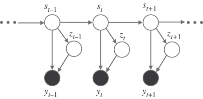
Figure 2 depicts the dependency between the variables as a graphical model. First of all, a hidden state at time t = 1, s₁, is determined by an initial state vector, π = [π₁, … ,π_J]^T, where π_j = p(s₁ = j). At time t, given a hidden state at the previous time step s_t−1, the current hidden state s_t depends only on s_t−1 and not on those at time t − 2 and before, i.e. the state transitions follow a Markov process: p(s_t|s_t−1, … , s₁) = p(s_t|s_t−1). By this (first-order) Markov property, the sequential dependency in the data is modelled. The state transition is determined by a transition matrix, A, where A_ij = p(s_t = j|s_t−1 = i). In this paper, the probability density of an observation, given a hidden state, is taken to be a finite mixture of Gaussians (MoG) as this offers the possibility of modelling arbitrarily complex multi-modal distributions (see [16] for example). Taking an MoG emission model introduces another set of hidden variables, Z = {z₁, … , z_T}, where z_t ∈ {1, … , K}, an indicator determining which mixture emission component is most responsible for observed y_t. Hence, the emission model has the following probability density for component k:

3.1

where μ_j is a mean value for the jth state and λ_jk is a precision (or inverse variance) value for the jth state and the kth component. Periods of distinctive behaviour of the laying hens can hence be identified using the HMM, as we interpret the variable s_t as dictating which state the observation y_t is generated from, namely normal or disturbance. Moreover, an MoG emission enables us to model heteroscedasticity, i.e. to identify observation sequences with differing variance structures, resulting in a model which is more robust against outliers, thus avoiding spurious state transitions.

Figure 2.

The graphical model of the HMM with a mixture of Gaussians emission probability. Filled and empty circles represent observations and hidden variables, respectively.

A HMM with an MoG emission has the following parameters: an initial state vector π, a state transition matrix A, a mixture component matrix C = [p(z_t = k|s_t = j)], a set of mean values μ = {μ_j} and a set of precision values Λ = {λ_jk}. Finding a solution for an HMM involves estimation of the parameters, θ = {π, A, C, μ, Λ}, as well as inference of the posterior distributions of the hidden variables, p(S, Z|Y). A two-stage algorithm is usually adopted, known as the Baum–Welch algorithm [17], which itself is a special case of the expectation–maximization (EM) algorithm [18]. However, the conventional EM algorithm has several limitations, most notably its inability to incorporate prior knowledge, its tendency to overfit and its difficulty in model selection.

In order to overcome these limitations, the variational Bayesian (VB) approach [19,20] is adopted in this paper. Given a model order ℳ = (J, K), the log marginal likelihood, log p(Y|ℳ), is approximated by maximizing a lower bound, which is referred to as the variational free energy after its original usage in the statistical physics literature¹. This quantity is maximized by the VB-EM algorithm where the VB-E and VB-M steps are alternately iterated until convergence. The maximization is equivalent to approximating the joint posterior of the parameters and the hidden variables. In Bayesian model selection, one selects the model order with the highest model posterior, p(ℳ|Y) ∝ p(Y|ℳ)p(ℳ). Assuming a flat prior over the model structure, i.e. p(ℳ) = const., leads to selecting the model order with the highest (negative) free energy.

Periods of distinctive behaviour can be identified by decoding the most probable path, {s*₁, … , s*_T}, resulting in a partition G_j = {t|s*_t = j}. The decoding is essentially equivalent to the Viterbi algorithm [13] with the only difference being that the ‘submarginalized’ parameter and likelihood are used. The VB learning algorithm for HMMs is presented in appendix 6. For more details, see Ji et al. [21] and Roberts & Penny [22].

3.2. State identification details

The optical flow datasets were log-transformed and a moving median filter was applied over the previous five samples to remove very short-term transients, lasting for one or two time steps. The success of the final predictive model is not sensitive to inclusion of this filter; its inclusion, however, is observed to improve the rate of convergence of the HMM. The data were normalized to have a zero mean and a unit variance, before the application of the HMM. Each frame was classified as normal or disturbance depending on which state it belonged to. In particular, since we know that disturbances are characterized by periods of higher activity, each frame was classified as normal if it was associated with the lowest mean activity hidden state and as a disturbance otherwise.

It is possible, of course, to apply supervised learning, e.g. binary classification, to the disturbance identification. However, this requires a significant amount of labelled data from both ‘classes’, normal and disturbance. For typical datasets, only a small fraction of data belong to the disturbance class, resulting in severe class imbalance. Moreover, labelled data are, in practice, often difficult, expensive and time-consuming to obtain, as they require the intensive efforts of human experts. We, therefore, focus on the development of unsupervised methodologies in this paper.

Figure 3 shows a typical example of an identification result on a section of data from a 27-week-old flock. The optical flows are close to zero (the global mean over all data) on the whole, but there is a clear increase, around t = 600. Bayesian model selection led to a model with two hidden states, J = 2, which are interpreted as normal and disturbance, and three components for the mixture model, K = 3. The HMM identified the disturbance period at the same location as the expert labelling. Although there are other very visible spikes in the optical flow, e.g. at t ≈ 530 and t ≈ 900, the HMM raised no false alarms, as transients in the optical flow were assigned to a high-variance non-disturbance state.

Figure 3.

Detection of a disturbance period in a section of typical optical flow dataset from a 27-week-old flock. The (blue) solid curve is the observation sequence while the (black) staircase plot is the estimated mean value of the hidden states. One standard deviation error bars are represented by the (pink) shading. The lower panel shows the expert labelling: zero for normal and one for disturbance.

The identification results on 19 such sections of data comprising 19 000 normal and disturbance events were compared with the expert labelling. Table 2 presents the resultant contingency table, where both the true positive and true negative rates were around 95 per cent. A χ²-test was carried out, using bootstrap undersampling so as to alleviate the severe class imbalance, with the null hypothesis that the cells in the table are evenly distributed. It was resoundingly rejected with a p-value of almost zero. We can conclude therefore that disturbance periods can be accurately identified by the methodology we present in this paper. As full state probabilities are returned by the model it is also possible to adjust the trade-offs between false positives and false negatives if there are unequal costs associated with them. In this paper, however, we take the cost associated with all misclassifications to be the same.

Table 2.

Contingency table of counts (percentages) for state identification results.

	estimated label
true label	disturbance	normal	total
disturbance	1797 (94.93)	96 (5.07)	1893
normal	366 (2.14)	16 741 (97.86)	17 107
total	2163	16 837	19 000

3.3. Disturbance measures

The HMM algorithm detailed in previous subsections was applied to each full-length recording with the model order (J, K) = (3, 3), which was determined by Bayesian model selection using the variational free energy over all datasets. Using the same model structure for all the datasets allows for easier collation and comparison of the results and avoids the computation required to evaluate a full set of models for each and every dataset. An example result is illustrated in figure 4. State 1 is designated as normal, while the other two as disturbances. For the jth state, for example, the mean value and its total duration are denoted by μ_j and τ_j, respectively. We derived three simple measures representing the disturbance profile as shown in table 3.

Figure 4.

A schematic of an identification result. Of T frames, three distinctive states were identified, one for normal and two for disturbance. The jth state lasted for τ_j frames with the mean value of μ_j.

Table 3.

Disturbance measures.

measure of disturbance	formula
frequency	(# disturbances)/T
proportion	(τ2 + τ3)/T
magnitude	(μ2 − μ1) · τ2/T + (μ3 − μ1) · τ3/T

4. Prediction of future feather damage

Our goal is to predict which flocks will develop severe feather damage. As described in §3, we derived a set of disturbance measures, which we will denote by the three-dimensional vector d. Another relevant and readily available piece of information is the age of each flock, a, when the video was taken. We define the interval, Δ, as being the time interval between the dates of video recording and future feather scoring. All variables, d, a, Δ) are used for predicting future feather scores. In other words, given the disturbance measures and the ‘video age’, a feather score will be predicted Δ days ahead. This section describes the prediction models employed and then presents the prediction results.

4.1. Prediction models

Consider a dataset of input–output instances, (X, f) = {(x_n, f_n)}, n = 1, … , N. An input vector consists of the disturbance measure d, the video age a, and the time interval Δ, i.e. . An output value corresponds to a future feather score. The number of instances available is 198, i.e. N = 198. We here consider two prediction models, one linear and the other nonlinear.

Linear regression (e.g. [23]) is one of the most popular regression models. Given an input vector x_*, the prediction is given by

4.1

where b₀ and b = [b₁, … , b_d]^T are d + 1 parameters to be estimated from the training data.

Gaussian processes (GPs; [24]) perform Bayesian inference by assuming a Gaussian distribution over the infinite numbers of possible outputs of the function to be estimated. A GP is specified by a mean vector, m, and a covariance matrix, K, over the function outputs:

4.2

where the covariance matrix is defined using a covariance function, i.e. K_nn′ = k(x_n, x_n′). In this paper, we adopt the squared exponential covariance function with additive independent output noise. The squared exponential covariance function offers a canonical model which is ideally suited to interpolating smooth functions with sparse data. The reader is pointed to, (e.g. [24]) for full discussion regarding the choice of covariance function.

4.3

where the hyperparameters σ_in and σ_out are the input and output length-scales, respectively. In the second term, σ_noise² is the output noise variance and δ(x, x′) is a Kronecker delta, which is one for x = x′ and zero otherwise.

When a new (test) input vector, x_*, is given, the joint prior distribution of the training outputs, f, and the test output, f_*, is

4.4

where k_*≡ [k(x_*, x₁), … , k(x_*, x_N)]^T. We can hence easily obtain the predictive distribution as a conditional Gaussian distribution:

4.5

where the mean and variance are expressed as follows:

4.6

and

4.7

The mean value, m_*, is usually taken as the point prediction, i.e. f̂_* = m_*.

Both models contain parameters or hyperparameters to be optimized. Their performance should be evaluated on a sample independent of the training data to avoid overfitting. As only 198 instances were available, leave-one-out validation was adopted to estimate performance on out-of-sample data. Specifically, a single instance from the dataset was assigned as the test data, and the remaining instances as the training data. A model is then trained using the training data and evaluated on the test data. This procedure is repeated for all possible choices of the test data.

In addition, since a feather score is a strictly positive quantity, each output value, f_n, was transformed to f̃_n = log(f_n + 1). A prediction m̃_* was made for f̃_* and then transformed to m_* = exp(m̃_*) − 1. For this reason, the error bars on the figures in the next subsection are asymmetric.

4.2. Prediction results

Feather scores depend on the birds' ages when the scores were recorded, since they tend to increase monotonically [11,25]. Figure 5 shows the GP fitting result based only on the age (=a + Δ). The relationship is slightly nonlinear although the prediction by linear regression (in a log scale) was not significantly different. Note that uncertainty increases, as expected, as the hens grow older. While this result shows an obvious relationship between ages and feather scores, better performance could be obtained using the disturbance measures in conjunction with age information.

Figure 5.

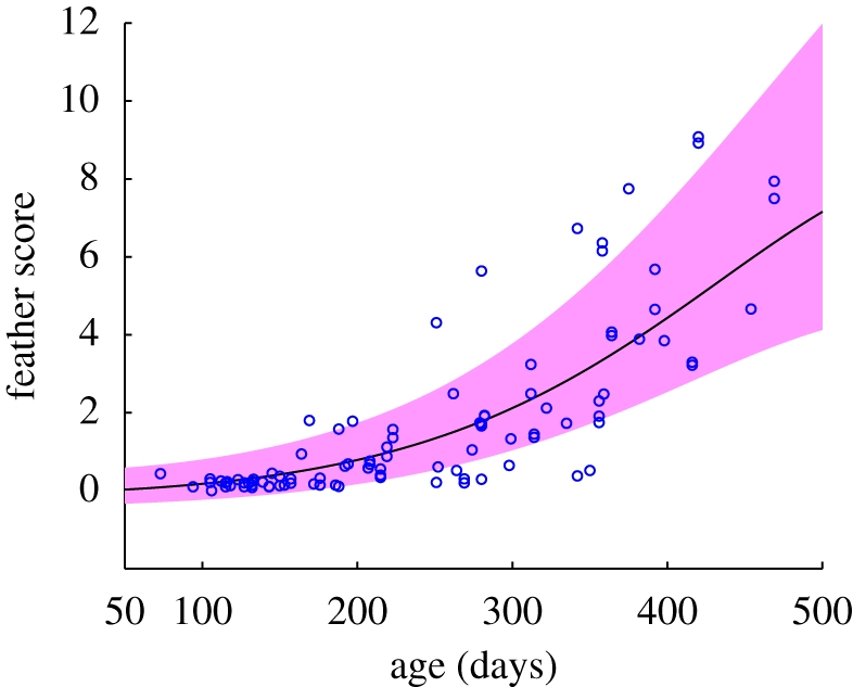
GP fitting of feather scores based only on ages. The (blue) circles represent the feather scores against ages, while the (black) curve and the (pink) shading are the GP prediction and its 1 s.d. error bar.

Figure 6 shows boxplots of absolute errors made by linear regression and Gaussian process regressors. For each model, two sets of input variables were compared: with age variables only (a and Δ) and with both the age variables and the disturbance measures. Linear regression performed slightly better with the disturbance measures, although the improvement was statistically insignificant according to a Brown–Forsythe test [26]. On the other hand, the GP was considerably better with the disturbance measures included. The variances of the errors were significantly different between the two sets of input variables with a p-value of less than 1 per cent (using the Brown–Forsythe test).

Figure 6.

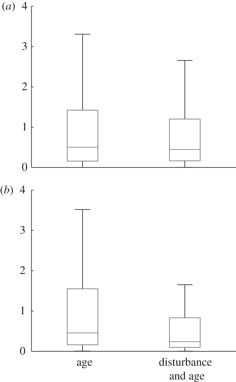
Boxplots of absolute errors by the two prediction models with respect to the input variables used. Each box has three lines at the lower quartile, median and upper quartile values, with the extended lines showing the range of the rest of the data. (a) Linear regression, (b) GP.

Table 4 lists the correlation coefficients between the true and the predicted feather scores with respect to the input variables used. Respectable performance was observed when the age variables were used. However, the best results were obtained using both sets of variables. The correlation coefficient of 0.8710 from the GP was higher than any other values with a p-value of less than 1 per cent according to a test based on Fisher's Z-transformation (e.g. [27]). Linear regression did not perform much better with the disturbance measures included, implying that the relationship between the disturbance measures and the (log) feather scores is nonlinear. Figure 7a shows an example plot of GP out-of-sample prediction for a 10-week-old flock as a function of prediction time. Figure 7b shows, for comparison, the GP output using age only as a predictive measure for future feather score.

Table 4.

Correlation coefficients between true and predicted feather scores. All the values are statistically significant with a p-value of 0.01 or lower.

variables	linear regression	GP
age	0.7197	0.7136
disturbance and age	0.7497	0.8710

Figure 7.

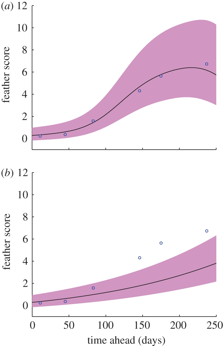
GP prediction results on a 10-week-old flock. The (blue) circles represent feather scores against the days ahead of the prediction. The (black) curves and the (pink) shadings are the predicted feather scores and their 1 s.d. error bars, respectively.

5. Discussion

Our results suggest that flocks at greatest risk of later developing severe feather damage can be recognized several weeks earlier using optical flow analysis of flock behaviour. Such prediction would be most valuable if it could be used to trigger the use of measures to prevent or control feather pecking, which is currently very difficult to do, especially if birds are not beak trimmed. However, being able to predict which flocks are most at risk might at least allow control measures such as lowered light levels or additional environmental enrichment to be targeted at these at-risk flocks, rather than used indiscriminately on all flocks—owing to cost or because some, such as straw bales or vegetation, are a biosecurity risk. Furthermore, detecting the early warning signs of severe feather pecking will be a valuable research tool in the search for more ethically acceptable ways of preventing and controlling feather pecking. As a caveat, it should be noted that the proposed method was used for predicting feather scores, not feather pecking itself. Feather pecking and feather scores, though closely related to each other, are not necessarily equivalent.

Optical flow measurements are now increasingly used for a range of applications such as monitoring traffic flow [28], the movement of glaciers [29], cell and sperm motility [30], the study of human crowds [31] and for studying groups of non-human animals [32]. Optical flow can be used both to track individuals and to recognize specific behaviour patterns [33], but its great advantage is that it can also be used to analyse the mass movements of whole groups such as herds, flocks or schools, where tracking individual animals is difficult or impossible. Whole frames or sections of frames, containing tens or hundreds of individuals can be assessed together and the basic statistical properties of these flow patterns can be derived automatically and continuously [34] using algorithms simple enough to deliver results continuously in real time. The flow patterns can of course potentially be analysed in many different ways and the key issue then becomes to find the appropriate statistical analysis that detects patterns of biological significance. In this particular case, we have shown that statistical anomalies detected by using HMM appear to be of significance to the future welfare of laying hens in that they appear to predict future feather damage before it has actually occurred. At risk flocks show signs of behavioural disturbance that this method is able to detect, but the method described here is only one of a range of possible models which have yet to be explored such as an HMM with an autoregressive (AR; [35]), or a generalized AR emission model [22] or even, a HMM with an infinite number of states [36]. We suggest that similar approaches might also be useful for early detection of other signs of poor welfare such as tail-biting in pigs or even subclinical signs of disease. Current research is investigating whether the spatial distribution of optical flow, on the image frames, improves the analysis. It also remains to be seen whether, on short timescales, these measures offer predictive information regarding the occurrence or prevalence of disturbance events.

All the methods considered in this paper were implemented using the Matlab programming language. Code for performing generic modelling using Bayesian dynamical models may be found under http://www.robots.ox.ac.uk/~parg/software.html.

6. Conclusions

This paper addresses the problem of predicting feather damage of laying hen flocks based on visual processing and statistical analysis. From video recordings, optical flows were extracted as indicators of the hens' movements. HMM were then applied to the optical flow datasets to identify disturbance periods and to derive the disturbance measures. Using these disturbance measures and age-related variables, feather scores were predicted via linear regression and nonlinear regression using Gaussian processes. It was shown that the Gaussian process model performed well and that the disturbance measures provided predictive information regarding future feather scores.

Appendix A. Variational Bayesian HMM

This section describes the VB learning algorithm for a HMM. First of all, the priors are defined as p(θ) = p(π)p(A)p(C)p(μ)p(Λ), each of which is to be conjugate, that is, Dirichlet for π, A and C, Gaussian for μ, and Gamma for Λ as follows:

A 1

A 2

A 3

A 4

A 5

where u^π, u^A, u^C, {w_j}, {r_j}, {ν_jk} and {v_jk} are hyperparameters, and 𝒟(·), 𝒩(·), 𝒢(·) denote the Dirichlet, Gaussian and Gamma distributions, respectively. The density functions and other relevant quantities of the distributions are given in appendix A.5.

A lower bound of a log marginal likelihood can be obtained using Jensen's inequality:

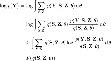A 6

The last term, F(q(S, Z, θ)), is called the variational free energy. It is easy to show that log p(Y) = F(q(S, Z, θ)) + KL(q(S, Z, θ)‖ p(S, Z, θ|Y)), where the KL(·‖·) is the Kullback–Leibler (KL) divergence between two distributions. Hence, maximizing F(q(S, Z, θ)) is equivalent to approximating p(S, Z, θ |Y) by q(S, Z, θ). For brevity, the model order, ℳ = (J,K), is omitted from all the conditional terms and assumed implicit.

Since approximation of the joint posterior is analytically intractable, the mean-field approximation is adopted, i.e. the approximate posterior can be factorized as

A 7

Consequently, the free energy is decomposed as

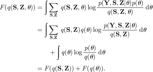A 8

The approximate posteriors are found using the VB-EM algorithm. The hidden variables part, F(q(S, Z)), is maximized in the VB-E step while the parameters part, F(q(θ)), is maximized in the VB-M step.

In the VB-E step, we have

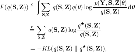A 9

where q★ (S, Z) ∝ exp[〈log p(Y, S, Z|θ)〉_q(θ)]. The relation means that the equality holds up to a constant, and 〈·〉_q(·) indicates an expectation with respect to the specified distribution. From equation (A 9), maximizing F(q(S, Z)) is equivalent to approximating q(S, Z) to q*(S, Z). Likewise, in the VB-M step, notating q(θ) = ∏_ℓ=1^L q(θ_ℓ), we have

A 10

The posterior of a parameter is approximated as

A 11

where θ_−ℓ denotes all the parameters excluding θ_ℓ. Since the conjugate priors are defined, q*(θ_ℓ) can be specified without actually computing the normalization terms. These two steps are iterated alternately until some terminating conditions. After finding the optimal model order, the most probable path of the hidden states is decoded. Algorithm 1 outlines the VB learning algorithm. The following subsections provide more detailed descriptions of the algorithm.

A.1. VB-E step

Suppose that the posteriors of the parameters are available from the previous iteration, that is, equations (A 19)–(A 23). Then, the ‘submarginalized’ likelihood for each observation, y_t, given a hidden state and a mixture component variables, is evaluated as

A 12

where 〈log λ_jk〉 is given in equation (B 7). A superscript of ‘(old)’ means that the posterior or the hyperparameter has been obtained in the previous iteration. A tilde (˜.) indicates an updated posterior hyperparameter, probability, or parameter obtained by marginalizing nuisance variables.

Algorithm 1.

The pseudo code for the VB learning algorithm for a HMM.

1:	INITIALIZATION
2:	Specify the model order, ℳ = (J,K).
3:	Define the prior hyperparameters. //Equations (A 1)–(A 5)
4:	REPEAT
5:	VB-E step to infer the hidden variables. //Section A.1
6:	VB-M step to estimate the posteriors of the parameters. //Section A.2
7:	Calculate the variational free energy, F. //Section A.3
8:	UNTILF is converged or the maximum number of iterations is reached.
9:	MODEL SELECTION
10:	Find the most probable model order. //Section A.4
11:	STATE IDENTIFICATION
12:	Find the most probable path of states. //Section A.5

Consider the following relation:

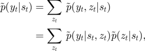A 13

where p̃(z_t|s_t) corresponds to C̃ = [C̃_jk] ∝ [exp(〈log C_jk〉)], given in equation (B 2). The forward and backward recursions are, respectively, as follows:

A 14

and

A 15

where α₁ ∝ p̃(y_t|s_t)p̃(s₁) and β_T = [1, … , 1]^T. The initial state probability, p̃(s₁), and the transition probability, p̃(s_t|s_t−1), correspond to π̃ = [π̃_j] ∝ [exp(〈log π_j〉)] and à = [Ã_ij] ∝ [exp(〈logA_ij〉)], respectively. Then, the posteriors of the hidden variables are now written as

A 16

A 17

A 18

A.2. VB-M step

The Dirichlet posteriors for the initial state, the transition, and the mixture component parameters are

A 19

A 20

A 21

The Gaussian posteriors for the mean values are

A 22

and

The Gamma posteriors for the precisions are

A 23

and

A.3. Variational free energy

The variational free energy is evaluated after each round of the two steps. From equation (A 8), the variational free energy can be expanded as

A 24

where the first term can be evaluated as

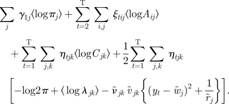A 25

The second term, the entropy of the hidden variables, is

A 26

The remaining terms associated to the KL divergences can be evaluated as given in equations (B 3), (B 5) and (B 8).

A.4. Model order selection

In Bayesian model selection, one selects a model order with the highest model posterior,

A 27

where p(Y|J, K), p(J, K) and p(Y) are the marginal likelihood, the model prior and the total evidence, respectively. Since the variational free energy is an approximation to the log-marginal likelihood, if we assume a flat model prior, that is, p(J, K) = const., ∀J, K, the model posterior is approximated as

A 28

In essence, we select a model order that leads to the highest free energy.

A.5. Decoding of the most probable path

The decoding of the most probable path of hidden states is essentially equivalent to the Viterbi algorithm described in [13]. The only difference is that we use the submarginalized parameter, Ã, and likelihood p̃(y_t|s_t) = exp[〈log p(y_t|s_t, z_t)〉 _{q^* (zt},_μ,Λ)].

Appendix B. Relevant distributions

This section presents the density functions, KL divergences and some relevant statistics for the Dirichlet, Gaussian and Gamma distributions.

B.1. Dirichlet distribution

For a variable , the Dirichlet density function with a parameter is

B 1

The expectation of the logarithm of the Dirichlet variable is

B 2

where ψ (·) is the digamma function. For two Dirichlet distributions, q(π) = 𝒟(π; ũ) and p(π) = D(π; u), the KL divergence is

B 3

B.2. Gaussian distribution

The Gaussian density function of is specified by a mean μ and a precision λ:

B 4

For two Gaussian distributions, q(y) = 𝒩(y;̃ μ, λ̃⁻¹) and p(y) = 𝒩(y; μ,λ⁻¹), the KL divergence is

B 5

B.3. Gamma distribution

For a variable , the Gamma density function with a shape parameter and a scale parameter is

B 6

The expectation of the logarithm of the Gamma variable is written as

B 7

For two Gamma distributions, q(λ) = 𝒢(λ; ν̃, ṽ) and p(λ) = 𝒢(λ; ν, v), the KL divergence is

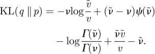B 8

References

- 1.Rodenburg T. B., van Hierden Y. M., Buitenhuis A. J., Riedstra B., Koene P., Korte S. M., van der Poel J. J., Groothuisd T. G. G., Blokhuis H. J. 2004. Feather pecking in laying hens: new insights and directions for research? Appl. Anim. Behav. Sci. 86, 291–298 [Google Scholar]
- 2.Dixon L. M. 2008. Feather pecking behaviour and associated welfare issues in laying hens. Avian Biol. Res. 1, 73–87 10.3184/175815508X363251 (doi:10.3184/175815508X363251) [DOI] [Google Scholar]
- 3.Blokhuis H. J., et al. 2007. The laywel project: welfare implications of changes in production systems for laying hens. Worlds Poult. Sci. J. 63, 101–114 10.1017/S0043933907001328 (doi:10.1017/S0043933907001328) [DOI] [Google Scholar]
- 4.Fossum O., Jansson D. S., Etterlin P. E., Vågsholm I. 2009. Causes of mortality in laying hens in different housing systems in 2001 to 2004. Acta Vet. Scand. 51, 3. 10.1186/1751-0147-51-3 (doi:10.1186/1751-0147-51-3) [DOI] [PMC free article] [PubMed] [Google Scholar]
- 5.Tauson R., Svensson S. A. 1980. Influence of plumage condition on the hen's feed requirement. Swedish J. Agric. Res. 10, 35–39 [Google Scholar]
- 6.El-Lethey H., Aerni V., Jungi T. W., Wechsler B. 2000. Stress and feather pecking in laying hens in relation to housing conditions. Br. Poult. Sci. 41, 22–28 10.1080/00071660086358 (doi:10.1080/00071660086358) [DOI] [PubMed] [Google Scholar]
- 7.Gentle M. J., Hunter L. N. 1991. Physiological and behavioural responses associated with feather removal in Gallus gallus var. domesticus. Res. Vet. Sci. 50, 95–101 [DOI] [PubMed] [Google Scholar]
- 8.Huber-Eicher B., Sebö F. 2001. Reducing feather pecking when raising laying hen chicks in aviary systems. Appl. Anim. Behav. Sci. 73, 59–68 10.1016/S0168-1591(01)00121-6 (doi:10.1016/S0168-1591(01)00121-6) [DOI] [PubMed] [Google Scholar]
- 9.Dennis R. L., Fahey A. G., Cheng H. W. 2009. Infrared beak treatment method compared with conventional hot-blade trimming in laying hens. Poult. Sci. 88, 38–43 10.3382/ps.2008-00227 (doi:10.3382/ps.2008-00227) [DOI] [PubMed] [Google Scholar]
- 10.Gentle M. J., Waddington D., Hunter L. N., Jones R. B. 1990. Behavioural evidence for persistent pain following partial beak amputation in chickens. Appl. Anim. Behav. Sci. 27, 149–157 10.1016/0168-1591(90)90014-5 (doi:10.1016/0168-1591(90)90014-5) [DOI] [Google Scholar]
- 11.Drake K. A., Donnelly C. A., Dawkins M. S. In press The influence of rearing and lay risk on propensity for feather damage in laying hens. Br. Poult. Sci. [DOI] [PubMed] [Google Scholar]
- 12.Dawkins M. S., Lee H., Waitt C. D., Roberts S. J. 2009. Optical flow patterns in broiler chicken flocks as automated measures of behaviour and gait. Appl. Anim. Behav. Sci. 119, 203–209 10.1016/j.applanim.2009.04.009 (doi:10.1016/j.applanim.2009.04.009) [DOI] [Google Scholar]
- 13.Rabiner L. R. 1989. A tutorial on hidden Markov models and selected applications in speech recognition. Proc. IEEE 77, 257–286 10.1109/5.18626 (doi:10.1109/5.18626) [DOI] [Google Scholar]
- 14.Beauchemin S. S., Barron J. L. 1995. The computation of optical flow. ACM Comput. Surveys 27, 433–467 10.1145/212094.212141 (doi:10.1145/212094.212141) [DOI] [Google Scholar]
- 15.Bright A., Jones T. A., Dawkins M. S. 2006. A non-intrusive method of assessing plumage condition in commercial flocks of laying hens. Anim. Welf. 15, 113–118 [Google Scholar]
- 16.Bishop C. M. 2006. Pattern recognition and machine learning. New York, NY: Springer [Google Scholar]
- 17.Baum L. E., Petrie T., Soules G., Weiss N. 1970. A maximization technique occurring in the statistical analysis of probabilistic functions of Markov chains. Ann. Math. Statist. 41, 164–171 10.1214/aoms/1177697196 (doi:10.1214/aoms/1177697196) [DOI] [Google Scholar]
- 18.Dempster A. P., Laird N. M., Rubin D. B. 1977. Maximum likelihood from incomplete data via the EM algorithm. J. R. Stat. Soc. Series B Stat. Methodol. 39, 1–38 [Google Scholar]
- 19.Jordan M. I., Ghahramani Z., Jaakkola T. S., Saul L. K. 1999. An introduction to variational methods for graphical models. Mach. Learn. 37, 183–233 10.1023/A:1007665907178 (doi:10.1023/A:1007665907178) [DOI] [Google Scholar]
- 20.Beal M. J., Ghahramani Z. 2003. The variational Bayesian EM algorithm for incomplete data. In Bayesian statistics, vol. 7 (eds Bernardo J. M., Bayarri M. J., Dawid A. P., Berger J. O., Heckerman D., Smith A. F. M., West M.), pp. 453–464 Oxford, UK: Oxford University Press [Google Scholar]
- 21.Ji S., Krishnapuram B., Carin L. 2006. Variational Bayes for continuous hidden Markov models and its application to active learning. IEEE Trans. Pattern Anal. Mach. Intell. 28, 522–532 10.1109/TPAMI.2006.85 (doi:10.1109/TPAMI.2006.85) [DOI] [PubMed] [Google Scholar]
- 22.Roberts S. J., Penny W. D. 2002. Variational Bayes for generalized autoregressive models. IEEE Trans. Signal Process. 50, 2245–2257 10.1109/TSP.2002.801921 (doi:10.1109/TSP.2002.801921) [DOI] [Google Scholar]
- 23.Johnson R. A., Wichern D. W. 1998. Applied multivariate statistical analysis, 4th edn Upper Saddle River NJ: Prentice-Hall [Google Scholar]
- 24.Rasmussen C. E., Williams C. K. I. 2006. Gaussian processes for machine learning. Cambridge, MA: MIT Press [Google Scholar]
- 25.Bright A. 2009. Time course of plumage damage in commercial layers. Vet. Rec. 164, 334–335 [DOI] [PubMed] [Google Scholar]
- 26.Brown M. B., Forsythe A. B. 1974. Robust tests for the equality of variances. J. Am. Statist. Assoc. 69, 364–367 10.2307/2285659 (doi:10.2307/2285659) [DOI] [Google Scholar]
- 27.Meng X., Rosenthal R., Rubin D. B. 1992. Comparing correlated correlation coefficients. Psychol. Bull. 111, 172–175 10.1037/0033-2909.111.1.172 (doi:10.1037/0033-2909.111.1.172) [DOI] [Google Scholar]
- 28.Bellomo N., Bianca C., Delitala M. 2009. Complexity analysis and mathematical tools towards the modelling of living systems. Phys. Life Rev. 6, 144–175 10.1016/j.plrev.2009.06.002 (doi:10.1016/j.plrev.2009.06.002) [DOI] [PubMed] [Google Scholar]
- 29.Giles A., Massom R. A., Warner R. 2009. A method for sub-pixel scale feature-tracking using Radarsat images applied to the Mertz Glacier Tongue, East Antarctica. Remote Sensing Environ. 113, 1691–1699 10.1016/j.rse.2009.03.015 (doi:10.1016/j.rse.2009.03.015) [DOI] [Google Scholar]
- 30.Shi L., Nascimento J., Chandsawangbhuwana C., Botvinick C., Berns M. 2008. An automatic system to study sperm motility and energetics. Biomed. Microdevices 10, 573–583 10.1007/s10544-008-9169-4 (doi:10.1007/s10544-008-9169-4) [DOI] [PMC free article] [PubMed] [Google Scholar]
- 31.Courty N., Corpetti T. 2007. Crowd motion capture. Comput. Animat. Virtual Worlds 18, 361–370 10.1002/cav.199 (doi:10.1002/cav.199) [DOI] [Google Scholar]
- 32.Bremond F., Thonnat M., Zuniga M. 2006. Video-understanding framework for automatic behavior recognition. Behav. Res. Methods 38, 416–426 [DOI] [PubMed] [Google Scholar]
- 33.Johansson A., Helbing D. 2008. From crowd dynamics to crowd safety: a video-based analysis. Adv. Complex Systems 11, 497–527 10.1142/S0219525908001854 (doi:10.1142/S0219525908001854) [DOI] [Google Scholar]
- 34.Sonka M., Hlavac V., Boyle R. 1999. Image processing, analysis, and machine vision. London, UK: PWS publishing. [Google Scholar]
- 35.Penny W. D., Roberts S. J. 1999. Dynamic models for nonstationary signal segmentation. Comput. Biomed. Res. 32, 483–502 10.1006/cbmr.1999.1511 (doi:10.1006/cbmr.1999.1511) [DOI] [PubMed] [Google Scholar]
- 36.Beal M. J., Ghahramani Z., Rasmussen C. E. 2002. The infinite hidden Markov model. In Advances in neural information processing systems (NIPS 2001), vol. 14 (eds Diettrich T., Becker S., Ghahramani Z.), pp. 577–584 Cambridge, MA: MIT Press [Google Scholar]