

Abstract
Shape analysis has become of increasing interest to the neuroimaging community due to its potential to precisely locate morphological changes between healthy and pathological structures. This manuscript presents a comprehensive set of tools for the computation of 3D structural statistical shape analysis. It has been applied in several studies on brain morphometry, but can potentially be employed in other 3D shape problems. Its main limitations is the necessity of spherical topology.
The input of the proposed shape analysis is a set of binary segmentation of a single brain structure, such as the hippocampus or caudate. These segmentations are converted into a corresponding spherical harmonic description (SPHARM), which is then sampled into a triangulated surfaces (SPHARM-PDM). After alignment, differences between groups of surfaces are computed using the Hotelling T2 two sample metric. Statistical p-values, both raw and corrected for multiple comparisons, result in significance maps. Additional visualization of the group tests are provided via mean difference magnitude and vector maps, as well as maps of the group covariance information.
The correction for multiple comparisons is performed via two separate methods that each have a distinct view of the problem. The first one aims to control the family-wise error rate (FWER) or false-positives via the extrema histogram of non-parametric permutations. The second method controls the false discovery rate and results in a less conservative estimate of the false-negatives.
1 Introduction
Quantitative morphologic assessment of individual brain structures is often based on volumetric measurements. Volume changes are intuitive features as they might explain atrophy or dilation due to illness. On the other hand, structural changes at specific locations are not sufficiently reflected in volume measurements. Shape analysis has thus become of increasing interest to the neuroimaging community due to its potential to precisely locate morphological changes between healthy and pathological structures.
One of the first and most influential research in shape analysis was presented by D’Arcy [1] in his ground-breaking book On Growth and Form. In more recent years, several researchers proposed shape analysis via deformable registration to a template ([2, 3, 4, 5]). Inter-subject comparisons are made by analyzing the individual deformable transformations. This analysis of the transformation fields has to cope with the high dimensionality of the transformation, the template selection problem and the sensitivity to the initial position. Nevertheless, several studies have shown stable shape analysis results. [6] and [7] presented some of the first mathematical methods for 3D shape analysis based on sampled descriptions. The shape analysis of densely sampled 3D Point Distribution Models (PDM) and their deformations was first investigated by [8]. Inspired by their experiments, [9] proposed shape analysis based on a parametric boundary description called SPHARM ([10]). The SPHARM shape analysis approach was extended by [11] to use the implied sampled surface (SPHARM-PDM), a method also used by [12]. [13, 14] and Golland [15] proposed shape analysis on medial shape descriptions in 3D and 2D, respectively. They used a fixed topology sampled model with implicit correspondence that is fitted to the objects.
This manuscript presents a comprehensive set of tools that form a pipeline for the computation of 3D structural statistical shape analysis on the object boundary via SPHARM (see Figure 1). It has been applied in several studies on brain morphometry, but can potentially be employed in other 3D shape analysis problems. The main limitations of our shape analysis methodology is the necessity of spherical topology.
Figure 1.

Schematic view of our SPHARM-PDM based shape analysis pipeline.
2 Methods
This section describes the SPHARM-PDM shape description, the statistical analysis methodology, as well as issue of alignment and scaling normalization.
In summary, the input of the proposed shape analysis is a set of binary segmentation of a single brain structure, such as the hippocampus or caudate. These segmentations are first processed to fill any interior holes and a minimal smoothing operation. The processed binary segmentations are converted to surface meshes, and a spherical parametrization is computed for the surface meshes using a area-preserving, distortion minimizing spherical mapping. The SPHARM description is computed from the mesh and its spherical parametrization. Using the first order ellipsoid from the spherical harmonic coefficients, the spherical parametrizations are aligned to establish correspondence across all surfaces. The SPHARM description is then sampled into a triangulated surfaces (SPHARM-PDM) via icosahedron subdivision of the spherical parametrization. These SPHARM-PDM surfaces are all spatially aligned using rigid Procrustes alignment. Group differences between groups of surfaces are computed using the standard robust Hotelling T2 two sample metric. Statistical p-values, both raw and corrected for multiple comparisons, result in significance maps. Additional visualization of the group tests are provided via mean difference magnitude and vector maps, as well as maps of the group covariance information.
The correction for multiple comparisons is performed via two separate methods that each have a distinct view of the problem. The first one aims to control the family-wise error rate (FWER) or false-positives via the extrema histogram of non-parametric permutations. The second method controls the false discovery rate and results in a less conservative estimate of the false-negatives.
2.1 SPHARM-PDM
In summary, the SPHARM description is a hierarchical, global, multi-scale boundary description that can only represent objects of spherical topology ([10]). The spherical parameterization is computed via optimizing an equal area mapping of the 3D voxel mesh onto the sphere and minimizing angular distortions. The basis functions of the parameterized surface are spherical harmonics. Each individual SPHARM description is composed of a set of coefficients, weighting the basis functions. [16] demonstrated that SPHARM can be used to express shape deformations. Truncating the spherical harmonic series at different degrees results in object representations at different levels of detail. SPHARM is a smooth, accurate fine-scale shape representation, given a sufficiently high representation level. Based on a uniform icosahedron-subdivision of the spherical parameterization, we obtain a Point Distribution Model (PDM).
Mathematics behind SPHARM
This section discusses the mathematical properties of the spherical harmonic basis functions. It gives a summary of spherical harmonic descriptors as they are presented in Brechbühler’s dissertation [17].
Spherical harmonic basis functions , −l ≤ m ≤ l of degree l and order m are defined on θ ∈ [0;π] × ϕ ∈ [0;2π) by the following definitions:
| (1) |
| (2) |
where denotes the complex conjugate of and the associated Legendre polynomials
| (3) |
Table 1 lists explicit expressions for the spherical harmonic functions up to degree 3. The Cartesian notion reveals that the spherical harmonics are polynomials in the 3D space (u0,u1,u2).
Table 1.
Explicit expressions of the spherical harmonics up to degree 3, in both polar and Cartesian form due to Brechbühler. The last part of the table gives the common normalizing constants, e.g.
| l | m = 0 | m = 1 | m = 2 | m = 3 |
|---|---|---|---|---|
| 0 | 1 | |||
| 1 | cosθ | eiφ sinθ |

|
|
| 2 | -1+3cos2θ | eiφ cosθ sinθ | e2iφ sin2θ | |
| 3 | -3cosθ+5cos3θ | eiφ (1-5cos2θ) sinθ | e2iφ cosθsin2θ | e3iφsin3θ |
|
| ||||
| 0 | 1 | |||
| 1 | u 2 | u0+iu1 |

|
|
| 2 | -1+3u22 | (u0+iu1)u2 | (u0+iu1)2 | |
| 3 | -3u2+5u23 | (u0+iu1)(1-5u22) | (u0+iu1)2u2 | (u0+iu1)3 |
|
| ||||
| 0 | ||||
| 1 | ||||
| 2 | ||||
| 3 | ||||
To express a surface using spherical harmonics, the three coordinate functions are decomposed and the surface takes the form
| (4) |
where the coefficients are three-dimensional vectors due to the three coordinate functions. The coefficients are obtained by solving a least-squares problem. Therefore, the values of the basis functions are gathered in the matrix Z = (zi, j(l,m)) with , where j(l,m) is a function assigning an index to every pair (l,m) and i denotes the indices of the nvert points to be approximated. The coordinates of these points are arranged in and all coefficients are gathered in . The coefficients that best approximate the points in least-squares sense are obtained by
| (5) |
Using spherical harmonic basis functions, we obtain a hierarchical surface description that includes further details as more coefficients are considered. This is illustrated in Fig. 2.
Figure 2.
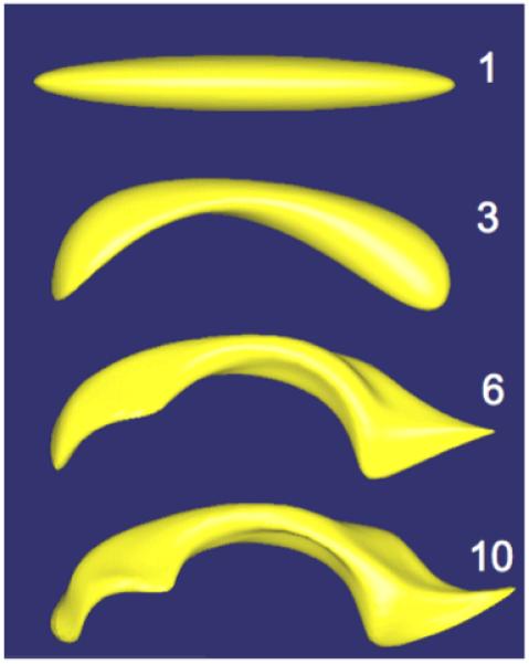
The SPHARM shape description of a human lateral ventricle shown at 4 different degrees ( 1, 3, 6, 10 harmonics).
SPHARM Correspondence
Correspondence of SPHARM-PDM is determined by normalizing the alignment of the spherical parameterization to an object-specific frame. In the studies presented in this paper, the normalization is achieved by rotation of the parameterization, such that the spherical equator, 0° and 90° longitudes coincide with those of the first order ellipsoid(see Figure 3). After this parametrization normalization, corresponding surface points across different objects possess the same parameterization.
Figure 3.
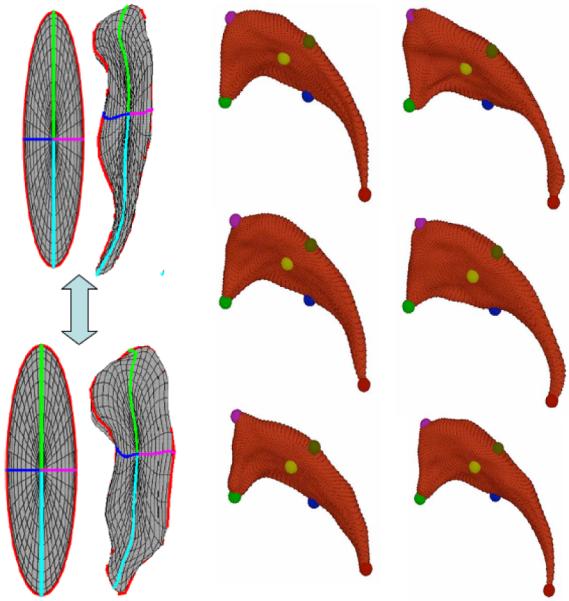
Left: Illustration of SPHARM correspondence via alignment of the spherical parametrization using the first order ellipsoid meridian and equator. Right: Set of 6 caudate structures with correspondence shown at selected locations via colored spheres.
The SPHARM-PDM shape analysis is visualized in Figure 1 using a caudate structure. Prior to the shape analysis, the group average object is computed for each subject group, and an overall average object is computed over all group average objects. Each average structure is computed by averaging the 3D coordinates of corresponding surface points across the group. The overall average object is then used in the shape analysis as the template object. At every boundary point for each object, we compute a distance map representing the signed local Euclidean surface distance to the template object. The sign of the local distance is computed using the direction of the template surface normal. In the global shape analysis, the average of the local distances across the whole surface is analyzed with a standard group mean difference test. The local shape analysis is computed by testing the local distances at every boundary point. This results in a significance map that represents the significance of these local statistical tests and thus allows locating significant shape differences between the groups. We corrected the shape analysis for the multiple comparison problem using a uniformly sensitive, non-parametric permutation test approach ([18]). The non-corrected significance map is an optimistic estimate of the real significance, whereas the corrected significance map is a pessimistic estimate that is guaranteed to control the rate of false positives at the given levelα (commonly α = 0.05) across the whole surface.
We have compared the SPHARM correspondence to other types of correspondences and it compared favourably to human expert established correspondence [19].
2.2 Area-preserving Spherical Mapping
The appropriate parameterization of the points of a surface description is a key problem for correspondence finding, as well as for an efficient SPHARM representation. Every point i on the surface is to be assigned a parameter vector (θi,ϕi) that are located on the unit sphere. A homogeneous distribution of the parameter space is essential for an efficient decomposition of the surface into SPHARM coefficients. We give here a brief summary of the surface parameterization procedure proposed by Brechbühler [10].
A bijective mapping of the surface to the unit sphere is created, i. e., every point on the surface is mapped to exactly one point on the sphere, and vice versa. The main idea of the procedure is to start with an initial parameterization. This initial parameterization is optimized so that every surface patch gets assigned an area in parameter space that is proportional to its area in object space. The initial mapping from surface to parameter space is constructed using discrete Laplace’s equations to solve the corresponding Dirichlet problem. To obtain a homogeneous distribution of the parameter space over the surface, this initial parameterization is modified in a constrained optimization procedure considering two criteria:
Area preservation: Every object region must map to a region of proportional area in parameter space.
Minimal distortion: Every quadrilateral should map to a spherical quadrilateral in parameter space.
Brechbühler establishes constraints for area preservation, while the distortion of the mesh serves as the objective function during optimization. The optimization solves the resulting system of nonlinear equations by linearizing them and taking Newton steps.
2.3 Surface Models from SPHARM: SPHARM-PDM
From the SPHARM description we can compute triangulated surfaces by sampling the spherical parameterization uniformly on the sphere. Equidistant sampling in the parameter space leads to a dense sampling around the poles (θ = 0, θ = π) and a coarse sampling around the equator (θ = π/2). This fact can be explained by the poles being mapped to all points having ϕ = 0...2π and θ = 0, or θ = π (see also Fig. 3). Using a linear, uniform icosahedron subdivision shown in Fig. 4, however, we gain a good approximation of a homogeneous sampling of the spherical parameter space and thus also of the object space. The subdivision is linear in the number of subdivisions along each edge of the original icosahedron, rather than the commonly used recursive subdivisions. Any recursive subdivision has a corresponding linear subdivision, but most linear subdivisions have no corresponding recursive subdivision (see Table 2).
Figure 4.

Icosahedron subdivision for different levels of sampling. From left to right: Base icosahedron, subdivision factors 2, 4 and 6.
Table 2.
Comparison of subdivision levels for recursive and linear subdivision of the icoshedron
| Recursive Level |
Linear Level |
Number of Surface Points |
|---|---|---|
| 1 | 1 | 12 |
| 2 | 2 | 42 |
| 3 | 4 | 162 |
| 4 | 8 | 642 |
| 5 | 16 | 2562 |
Using the pre-computed parameter locations (θi,ϕi) from the icosahedron subdivision, we can compute the PDM directly from the coefficients, as the parameter locations stay constant for all objects at a given subdivision level. The sampling points at the locations (θi,ϕi) are obtained using equation (4):
In our experience the sampling for the surface of brain structures should be chosen between subdivision level 10 (1002 surface points) and 20 (4002 surface points) depending on the complexity of the objects. For example, hippocampal surfaces are well represented by a subdivision level 10 and caudate surfaces by a subdivision level 15.
2.4 Alignment and Scaling Normalization
Alignment and scaling of the objects are two important issues in shape analysis that are also discussed here [11]. In general, we usually chose rigid-body Procrustes alignment ([20]) followed by no scaling normalization or scaling inversely to the intra-cranial cavity volume (ICV). Commonly both results are reported in a shape analysis study, the original scale analysis represents an unbiased raw analysis, whereas the ICV scale analysis corrects for differences in overall interior head size and thus approximatively normalizes for gender and age differences. In general both types of analysis should yield similar patterns of differences and special care needs to be taken if this is not the case.
2.5 Local Testing of Group Mean Difference using Hotelling T2 metric
After shape description, correspondence establishment, alignment and scaling normalization, the next step in the shape analysis pipeline consists of testing for differences between groups at every surface location (see Figure 5). This can be done in 2 main fashions:
Analyzing the magnitude of the local difference vector to a template: For this option, a template needs to be first selected, usually this is the common mean of the 2 groups or the mean of separate control group. The magnitude of the difference is easily understood and results in difference maps for each subject. Also, the resulting univariate statistical analysis is quite well known and local significance can be easily computed using the Student t metric. The main disadvantage of this method is the need to select a template, which introduces an additional bias into the statistical analysis. We applied this method in earlier studies of hippocampi [21] and ventricles [22].
Analyzing the spatial location of each point: For this option, no template is necessary and multivariate statistics of the (x,y,z) location is necessary. We have chosen to use the Hotelling T2 two sample difference metric as a measurement of how 2 groups locally differ from each other. The standard Hotelling T2 is defined as , where Σ = (Σ1(n1 - 1) + Σ2(n2 - 1))/(n1 + n2 - 2) is the pooled covariance matrix. An alternative modified Hotelling T2 metric is less sensitive to group differences of the covariance matrixes and the number of samples[23]: . All our current studies are based on this modified Hotelling T2 metric.
Figure 5.

Left: Schematic view of testing procedure: A set of features per surface point (shown as colormaps) are analyzed using uni- or multi-variate statistics, resulting in a raw significance map (bottom) .Right: The raw significance maps are overly optimistic and need to be corrected to control for the multiple comparison problem. The corrected significance maps on the other hand are commonly pessimistic estimates.
We then want to test the two groups for differences in the means of the selected difference metric (univariate: Student t, multivariate: Hotelling T2) at each spatial location. Permutation tests are a valid and tractable approach for such an application, as they rely on minimal assumptions and can be applied even when the assumptions of the parametric approach are untenable. Non-parametric permutation tests are exact, distribution free and adaptive to underlying correlation patterns in the data. Further, they are conceptually straightforward and, with recent improvements in computing power, are computationally tractable.
Our null hypothesis is that the distribution of the locations at each spatial element is the same for every subject regardless of the group. Permutations among the two groups satisfy the exchangeability condition, i.e. they leave the distribution of the statistic of interest unaltered under the null hypothesis. Given n1 members of the first group ak, k = 1...n1 and n2 members of the second group bk, k = 1...n2, we can create permutation samples. A value of M from 20000 and up should yield results that are negligibly different from using all permutations [24].
2.6 Correction for Multiple Comparison
The local shape analysis involves testing from a few to many thousands of hypothesis (one per surface element) for statistically significant effects. It is thus important to control for the multiple testing problem (see Figure 5), and the most common measure of multiple false positives is the familywise error rate (FWER). The multiple testing problem has been an active area of research in the functional neuroimaging community. The most widely used methods in the analysis of neuroimaging data use random field theory [25] [26] and make inferences based on the maximum distribution. In this framework, a closed form approximation for the tail of the maximum distribution is available, based on the expected value of the Euler characteristic of the thresholded image [26]. However, random field theory relies on many assumptions such as the same parametric distribution at each spatial location, a point spread function with two derivatives at the origin, sufficient smoothness to justify the application of the continuous random field theory, and a sufficiently high threshold for the asymptotic results to be accurate.
In our work, we are employing non-parametric permutation tests and false discovery rate as two alternative correction methods for the multiple comparison problem.
Minimum over Non-parametric permutation tests
Non-parametric methods deal with the multiple comparisons problem [18] and can be applied when the assumptions of the parametric approach are untenable. Similar methods have been applied in a wide range of functional imaging applications [27, 28, 29].
Details of this method are described in [18] and only a summary is provided here. The correction method is based on computing first the local p-values using permutation tests. The minimum of these p-values across the surface is then computed for every permutation. The appropriate corrected p-value at level α can then be obtained by the computing the value at the α-quantile in the histogram of these minimum values. Using the minimum statistic of the p-values, this method correctly controls for the FWER, or the false positives, but no control of the false negatives is provided. The resulting corrected local significance values can thus be regarded as pessimistic estimates akin to a simple Bonferroni correctection.
False Discovery Rate
Additionally to the non-parametric permutation correction, we have also implemented and applied a False Discovery Rate Estimation (FDR) [30, 31] method. The innovation of this procedure is that it controls the expected proportion of false positives only among those tests for which a local significance has been detected. The FDR method thus allows an expected proportion (usually 5%) of the FDR corrected significance values to be falsely positive. The correction using FDR provides an interpretable and adaptive criterion with higher power than the non-parametric permutation tests. FDR is further simple to implement and computationally efficient even for large datasets.
The FDR correction is computed as follows [31]:
Select the desired FDR bound q, e.g. 5%. This is the maximum proportion of false positives among the significant tests that you are willing to tolerate (on average).
Sort the p-values smallest to largest.
Let pq be the p-value for the largest index i of the sorted p-values psort,i ≤ q · i/N, where N is the number of vertices.
Declare all locations with a p-value p ≤ pq significant.
3 Computation scheme and Implementation
This section describes the set of shape analysis tools and the use of these in succession to compute the whole shape analysis (see Figure 7). The general workflow starts from the segmented datasets with binary labels for each structure of interest. The SegPostProcess program extracts a single binary label and applies heuristic methods to ensure the spherical topology of the segmentation. In the next step, the GenParaMesh computes the surface mesh corresponding to the segmentation, as well as a spherical parametrization of this surface mesh via area preserving mapping (see Section 2.2). The SPHARM-PDM shape representation is then computed using the ParaToSPHARMMesh program, which also handles issues of alignment. These three programs have to be run on all datasets in a shape analysis study. Often they are applied in parallel to the datasets. After all SPHARM-PDM representations have been computed, the statistical testing program StatNonParamTestPDM computes the difference maps, the significance maps, as well as the descriptive statistics such as the mean surfaces and covariance matrixes,
Figure 7.

Workflow of the shape analysis pipeline starting at the segmentation of the brain structures to the local final statistical analysis.
All these tools are command line tools without any graphical user interface. They have an online help/usage describing the input and output parameter specification. This information is printed on the terminal window by calling the program without any parameters or using the ’-help’ option.
All input and output meshes are stored in ITK-readable format of an itk::MeshSpatialObject. Conversion tools to/from other formats, such as OpenInventor and STL are also provided.
3.1 Processing of Binary Labels: SegPostProcess
The application of the SegPostProcess program is optional and but we recommend its use, as it ensure spherical topology of the segmentation and offers a series of services:
Extraction of a single label or a label range: This is especially helpful if the label dataset contains multiple labels.
Resampling of the label data: Segmentation data from MRI or other modalities are often stored at rather coarse resolution or at non-isotropic resolution. The input to GenParaMesh has to be of isotropic resolution and a relative fine resolution is recommended. In our studies, we have commonly resampled the data to an isotropic resolution of 0.5 mm to 0.75 mm.
Spherical topology: Any cavities fully enclosed in the segmentation is filled, two smoothing operations are applied, a full 6-connectedness is ensured, and only the largest component in the image is extracted. The cavity filling only fills fully interior structures and thus leaves the exterior boundary unedited. The first smoothing operation is implemented via a binary closing operation and the second smoothing operation is a level set based anti-alias smoothing (ITK filter itk::AntiAliasBinaryImageFilter [32]).
A common use of this tool is illustrated by the following command line. The output is a single label dataset.
SegPostProcess Label.hdr -o Label_PP.hdr -label 1-space 0.75,0.75,0.75
3.2 Spherical Parametrization: GenParaMesh
GenParaMesh first extracts the surface of the input label segmentation by following the ’cracks’ between the voxels of the foreground (label) and the background. The resulting mesh coordinates are thus off by minus half a voxel-width from coordinate systems that place the origin at the center of the voxels. This surface mesh is mapped to sphere using the methods described in Section 2.2. If the tool reports a bad Euler number, then this shows that the extracted surface is not of spherical topology, whereas the vice versa is not necessarily true. An indication of a successful parametrization is given by the output line ’initially active:’. If the number of initially active equations is low, a successful computation is likely. In our experience, less than 2% of the datasets do not finish successfully when SegPostProcess is first applied with a reasonably high resolution.
A common use of this tool is illustrated by the following command line. The output is two meshes, one for the surface and one for the spherical parametrization.
GenParaMesh Label_PP.hdr -iter 800 -label 1
3.3 SPHARM-PDM: ParaToSPHARMMesh
This tool computes the SPHARM-PDM representation and resolves issues of correspondence and alignment. The input is a surface mesh with spherical parametrization. It is not necessary that this parametrization has been computed using our GenParaMesh, but other parametrizations can equally be used, such as conformally mapped spherical parametrizations. As a first step, the raw spherical harmonic coefficients are computed only up to the first degree and the first order ellipsoid is determined. The spherical parametrization is then rotated such that the poles of the first order ellipsoid are coinciding with the poles of the parametrization. The spherical harmonic coefficients are recomputed up to the degree specified on the command line option. Additionally, the surface points of the SPHARM are reconstructed using the icosahedron subdivision scheme described in section 2.3.
The two main parameters of this tool are the maximal degree for the SPHARM computation and the subdivision level for the icosahedron subdivision. In our experience, the SPHARM maximal degree is should be chosen between 12 (hippocampus) to 15 (lateral ventricle, caudate) for brain structures. If the degree is chosen too high the reconstructed SPHARM surface will often show signs of voxelization. By using the ’-paraOut’ command line option, the spherical icosahedron subdivision, as well as local phi and theta attribute files for the quality control visualization with KWMeshVisu are written out.
Correspondence: The SPHARM shape description has an object-inherent correspondence based on the first order ellipsoid. Unfortunately this is not fully unique as the first order ellipsoid can be flipped along any of its axis with the same result. Thus, without additional measures the correspondence is ambiguously defined in regard to flips along these axis. In order to clarify this ambiguity, an additional SPHARM object (described by SPHARM coefficients) can be provided as a flip-template. This flipTemplate is used to test all possible flips of the parametrization along the first order ellipsoid axis and select the one whose reconstruction has minimal distance to the flip-template. Commonly, the first object is computed without providing a flip-template and then serves for all subsequent objects as the flip-template (see also Section 4).
Alignment: The ParaToSPHARMMesh tool provides two types of alignment. The first type performs an alignment of the normalized first order ellipsoid axis to the unit-axis with the ellipsoid center located at the origin. The second alignment type is a rigid-body Procrustes alignment [6], i.e. Procrustes alignment only with translation and rotation. Whereas the first alignment is object inherent, the Procrustes alignment is in need of a template, which can optionally be supplied.
A common use of this tool is illustrated by the following command line. The output is a series of SPHARM coefficients and SPHARM-PDM meshes, one set in the original coordinate system, one in the first order ellipsoid aligned coordinate system and one in the Procrustes aligned coordinate system.
ParaToSPHARMMesh Label_surf.meta Label_para.meta -subdivLevel 10 -spharmDegree 12 \
-flipTemplate template.coef -regTemplate template.meta
3.4 Statistics: StatNonParamTestPDM
Once all SPHARM-PDM meshes have been computed, group differences of the local surface point distributions can be assessed using the StatNonParamTestPDM. There are two main types of results from the statistical testing step: a) descriptive group statistics, such as the mean and covariance information, and b) group mean difference hypothesis testing. The descriptive statistics are used for quality control, sanity check, as well as these are necessary to make sense of the computed significance maps (”Is that significant region enlarged in the patient population?”). The significance maps show the regions of significant difference of the Hotelling T2 metric with 3 different maps (see also section 2.5): the raw p-value map, the FDR corrected p-value map, and the permutation based corrected p-value map. The value of the Hotelling T2 metric is also useful to visualize the full range of the effect size.
The current version of the tool also computes a single global shape difference by averaging the local Hotelling T2 metric across the whole surface. The p-value is computed the same way as for the local tests using non-parametric permutation tests. No correction is needed for the global shape difference as only a single test is performed. Additional other measures of global shape difference will be implemented, such as percentile measures of the Hotelling T2 representing stable estimations of extremal difference, such as the 68% and 95% percentiles.
The main parameter of the testing procedure is the number of permutations employed for both the computation of the raw and corrected p-values. As a rule of thumb, we are employing 10 times the number of surface mesh points, which is a safe estimate and results in quite extensive computation and memory requirements. Other relevant parameters include the maximal significance threshold (commonly chosen at 5%), as well as the resolution of the significance correction captured by the number of thresholds uniformly spaced between null and the maximal significance threshold (a good value is about 1000). For example, a maximal threshold of 5% with 10 threshold steps results in a correction resolution of 5%/10 = 0.5%. The number of steps parameter does not affect the raw significance map, which is rather determined by the number of permutations.
The StatNonParamTestPDM tool has several options for specifying its input. There are 2 main input types: a) text file listing all mesh files with corresponding information b) text file containing raw feature information. Using the second option, the tool can be applied to many different types of data that are embedded in a linear space, but limited descriptive group statistics are provided. The first option is simpler to use and has a richer set of output. Both options use ASCII text files, which reserve a single line per subject. For the mesh-list file, each line contains first the group identifier number (often either 0 or 1), then the scaling factor for an optional scaling normalization, followed by the absolute or relative path to the mesh-file. The scaling normalization is only performed when the appropriate ’-scale’ command line option is also present, otherwise the scaling information is simply omitted.
In case, data other than meshes are to be tested, the current version of the program allows the testing of univariate, bi and tri-variate data via the ’-2DvectorData’ and ’-3DvectorData’ options. Additional information needs to be provided, identifying the column numbers (indexed at 0) for the group identification number and for the first feature, as well as the numbers of features.
A common use of this tool is illustrated by the following command line. The output is are mean surface meshes for both groups and for all datasets, as well as attribute files for Covariance statistics, mean difference, local significance, and Hotelling T2 values. Additionally the significance of the global shape difference is written out.
StatNonParamTestPDM listfile.txt -out stats -surfList -numPerms 20000 \
-signLevel 0.05 -signSteps 1000
3.5 Visualization using KWMeshVisu
We have also developed a tool for the intuitive visualization of the statistical results, as well as for inspecting the established SPHARM correspondence. This tool is called KWMeshVisu and the SPHARM-PDM and statistical visualizations in this document have been created with it. The use and implementation details of this tool have been described in a separate paper, which has been submitted to the ISC/NAMIC Workshop on open science at MICCAI 2006.
3.6 Download and Installation
The shape analysis framework described in this paper is both accessible through the Sandbox of the National Alliance for Medical Image Computing NAMIC or directly as part of the UNC NeuroLib library [33]. Instructions for the download and installation process of the UNC NeuroLib can be found in the tutorial section. For compilation ITK libraries as well as lapack and blas libraries are necessary. Lapack and blas are often installed standardly on UNIX system, or can be downloaded from www.netlib.org/lapack.
4 Results
As exemplary test study we applied our shape analysis framework to a schizo-typal personality disorder (SPD) study on the caudate brain structure that was available to us through the NAMIC network [34]. The data consists of structural SPGR MRI datasets from 15 right handed medication-free male SPD patient, as well as from 14 matched healthy control subjects. Although both left and right hemispheric caudate were outlined on the MRI data, only the right caudate is presented here as a test study. Additionally, we are currently developing appropriate 3D synthetic test datasets, which will be published online as open access data.
The following simple script was used for the computation of the SPHARM-PDM descriptions:
#!/bin/tcsh -f
foreach case (/Data/caud*/*_R.gipl)
set ppcase = $case:r_pp.gipl
SegPostProcess $case -o $ppcase-label 1 -space 0.5,0.5,0.5
GenParaMesh $ppcase -iter 1000 -label 1
set meshPrefix = $ppcase:r
ParaToSPHARMMesh ${meshPrefix}_surf.meta ${meshPrefix}_para.meta \
-subdivLevel 15 -spharmDegree 15 \
-flipTemplate flipTemplate.coef -regTemplate regTemplate.meta
end
The correspondence of the SPHARM-PDM description was visually controlled (see Figure 8) for all datasets. For the group mean difference testing step, a text files was created listing the names of all mesh-files preceded by the group identifier (either 0 or 1) and the scaling factor. In this case the scaling factor was 1.0 for all cases, i.e. no scaling was performed. A sample line in this mesh list text-file thus looks like the following:
1 1.0 /Data/caud1/caud1_R_pp_surfSPHARM_procalign.meta
Figure 8.

Quality Control visualization of the SPHARM correspondence with KWMeshVisu using the Phi-attribute file shown on 3 randomly selected cases. Same color represent the same ϕ parameter value of the spherical parametrization.
This mesh list file was then the input of the statistical testing program, called in the following fashion:
StatNonParamTestPDM caudList.txt -out stats -surfList -numPerms 20000 \
-signLevel 0.05 -signSteps 1000
The descriptive group statistics (see Figure 9) show that the mean objects of the 2 groups are quite similar. The differences between the mean are overall small (max at 1.6 millimeter), but most pronounced in the anterior head region, the superior body region and the posterior tail region 1. The visualization of the covariance ellipsoids show that the variability is reduced in the body section compared to the anterior head and especially the posterior tail section.
Figure 9.

Descriptive statistics of right caudate analysis. The left visualization shows the mean difference as a colormap from green (0 mm difference) to red (1.6 mm difference) as well an vectorfield on the overall mean surface mesh. For two regions with large differences a zoomed view is provided. The right visualization shows the covariance ellipsoid colored with the magnitude of the largest ellipsoid axis (axis of largest covariance). The same two zoomed views are provided. The variance in the first zoom section is markedly reduced compared to the second zoom section.
The results of the mean difference hypothesis tests are visualized in Fiigure 10. The raw significance maps displays an overly optimistic estimate with the superior body, as well as anterior head region to be significantly different. The conservative, permutation based correction map provides a pessimistic estimate with only a single significant region in the anterior head region. The result of the false discovery rate correction is in-between the raw and the permutation based correction. On one hand, Significant parts in the anterior tail section are visible in the raw significant map, but are not preserved in the FDR corrected map. On the other hand, significant parts in the superior body as well as the anterior head region are present in the FDR corrected maps. The global shape difference has a p-value of p = 0.009.
Figure 10.

Significance testing on right caudate study
Based on these results, a significant shape difference between the two populations on the right caudate is clearly suggested. The main differences are enlarged section in controls compared to SPD located in the anterior head and superior body regions. For a full shape analysis, we recommend to both analyze the objects in their original scale (scaling factor = 1.0, as in this study), as well as normalized for the individual intra-cranial cavity volume (ICV). The ICV is usually acquired in a separate brain tissue segmentation and the scaling factor f is then chosen as . As this study serves as an example of how to employ our shape analysis framework, the analysis of the ICV normalized data is omitted here.
5 Conclusion
We have presented a comprehensive, local shape analysis framework founded on the SPHARM-PDM shape representation and local permutation tests. The whole software is available as open source and is currently in use by several research groups outside of UNC.
We presented research and software development in progress, and many additional enhancements of the current tool base are being developed or are planned. These enhancements include the incorporation ofsubject covariates, such as age, gender, handedness etc, as well as an user-interface based control tool for the whole shape analysis.
Figure 6.

Left: Scheme of P-value computation via permutation tests. The real group difference S0 (e.g. Hotelling T2) is compared to that the group differences Sj of random permutations of the group labels. The quantile in the Sj histogram associated with S0 is the p-value. Right: Example run on test data with 1000 random permutations. On the left the individual Sj are plotted and on the left the corresponding Sj histogram is shown. The black line indicates the value of S0.
6 Acknowledgment
We are thankful to Steve Pizer and Sarang Joshi for highly valuable discussions in regard to shape analysis. This research has been/is supported by the UNC Neurodevelopmental Disorders Research Center HD 03110, NIH Roadmap for Medical Research, Grant U54 EB005149-01, NIH NIBIB grant P01 EB002779, EC-funded BIOMORPH project 95-0845, Department of Veteran Affairs Merit Award, VA Research Enhancement Award Program, NIH R01 MH50747, and K05 MH070047.
Footnotes
The naming of caudate head and tail regions in this section are not based on anatomical labels
References
- [1].Thomson D. On Growth and Form. second edition. Cambridge University Press; 1942. 1. [Google Scholar]
- [2].Davatzikos C, Vaillant M, Resnick S, Prince JL, Letovsky S, Bryan RN. A computerized method for morphological analysis of the corpus callosum. J. of Comp. Assisted Tomography. 1996 Jan./Feb;20:88–97. doi: 10.1097/00004728-199601000-00017. 1. [DOI] [PubMed] [Google Scholar]
- [3].Joshi S, Miller M, Grenander U. On the geometry and shape of brain sub-manifolds. Pat. Rec. Art. Intel. 1997;11:1317–1343. 1. [Google Scholar]
- [4].Csernansky JG, Joshi S, Wang LE, Haller J, Gado M, Miller JP, Grenander U, Miller MI. Hippocampal morphometry in schizophrenia via high dimensional brain mapping. Proc. Natl. Acad. Sci. USA. 1998 September;95:11406–11411. doi: 10.1073/pnas.95.19.11406. 1. [DOI] [PMC free article] [PubMed] [Google Scholar]
- [5].Csernansky JG, Joshi S, Wang LE, Haller J, Gado M, Miller JP, Grenander U, Miller MI. Hippocampal morphometry in schizophrenia via high dimensional brain mapping. Proc. Natl. Acad. Sci. USA. 1998 September;95:11406–11411. doi: 10.1073/pnas.95.19.11406. 1. [DOI] [PMC free article] [PubMed] [Google Scholar]
- [6].Bookstein FL. Shape and the Information in Medical Images: A Decade of the Morphometric Synthesis. Comp. Vision and Image Under. 1997 May;66(2):97–118. 1, 3.3. [Google Scholar]
- [7].Dryden IL, Mardia KV. Multivariate shape analysis. Sankhya. 1993;55:460–480. 1. [Google Scholar]
- [8].Cootes T, Taylor CJ, Cooper DH, Graham J. Active shape models - their training and application. Comp. Vis. Image Under. 1995;61:38–59. 1. [Google Scholar]
- [9].Gerig G, Styner M, Shenton ME, Lieberman JA. Shape versus size: Improved understanding of the morphology of brain structures; MICCAI; 2001; pp. 24–32. 1. [Google Scholar]
- [10].Brechbühler C, Gerig G, Kübler O. Parametrization of closed surfaces for 3-D shape description. Comp. Vision, Graphics, and Image Proc. 1995;61:154–170. 1, 2.1, 2.2. [Google Scholar]
- [11].Gerig G, Styner M, Jones D, Weinberger D, Lieberman J. Shape analysis of brain ventricles using spharm; MMBIA; IEEE press. 2001; pp. 171–178. 1, 2.4. [Google Scholar]
- [12].Shen L, Ford J, Makedon F, Saykin A. SPIE-Medical Imaging. 2003. Hippocampal shape analysis surface-based representation and classification. 1. [Google Scholar]
- [13].Pizer S, Fritsch D, Yushkevich P, Johnson V, Chaney E. Segmentation, registration, and measurement of shape variation via image object shape. IEEE Trans. Med. Imaging. 1999 Oct.18:851–865. doi: 10.1109/42.811263. 1. [DOI] [PubMed] [Google Scholar]
- [14].Styner M, Gerig G, Lieberman J, Jones D, Weinberger D. Statistical shape analysis of neuroanatomical structures based on medial models. Medical Image Analysis. 2003;7(3):207–220. doi: 10.1016/s1361-8415(02)00110-x. 1. [DOI] [PubMed] [Google Scholar]
- [15].Golland P, Grimson WEL, Kikinis R. Statistical shape analysis using fixed topology skeletons: Corpus callosum study; IPMI; 1999; pp. 382–388. 1. [Google Scholar]
- [16].Kelemen A, Székely G, Gerig G. Elastic model-based segmentation of 3d neuroradiological data sets. IEEE Trans. Med. Imaging. 1999 October;18:828–839. doi: 10.1109/42.811260. 2.1. [DOI] [PubMed] [Google Scholar]
- [17].Brechbühler C. Description and Analysis of 3-D Shapes by Parametrization of Closed Surfaces. 1995. Diss., IKT/BIWI, ETH Zürich, ISBN 3-89649-007-9. 2.1. [Google Scholar]
- [18].Pantazis D, Leahy RM, Nichol TE, Styner M. Statistical surface-based morphometry using a non-parametric approach; Int. Symposium on Biomedical Imaging(ISBI); April 2004; pp. 1283–1286. 2.1, 2.6. [Google Scholar]
- [19].Styner M, Rajamani K, Nolte LP, Zsemlye G, Szekely G, Taylor C, Davies RH. Evaluation of 3d correspondence methods for model building; IPMI; July 2003; pp. 63–75. 2.1. [DOI] [PubMed] [Google Scholar]
- [20].Bookstein FL. Morphometric Tools for Landmark Data: Geometry and Biology. Cambridge University Press; 1991. 2.4. [Google Scholar]
- [21].Styner M, Lieberman JA, Pantazis D, Gerig G. Boundary and medial shape analysis of the hippocampus in schizophrenia. Medical Image Analysis. 2004;8(3):197–203. doi: 10.1016/j.media.2004.06.004. 2.5. [DOI] [PubMed] [Google Scholar]
- [22].Styner M, Lieberman JA, McClure RK, Weingberger DR, Jones DW, Gerig G. Morphometric analysis of lateral ventricles in schizophrenia and healthy controls regarding genetic and disease-specific factors. Proceedings of the National Academy of Science, PNAS. 2005;102(12):4872–4877. doi: 10.1073/pnas.0501117102. 2.5. [DOI] [PMC free article] [PubMed] [Google Scholar]
- [23].Seber GAF. Multivariate Observations. John Wiley & Sons; 1984. 2.5. [Google Scholar]
- [24].Edgington ES, editor. Randomization Tests. Academic Press; 1995. 2.5. [Google Scholar]
- [25].Chung MK. Ph.D. thesis. McGill University; Montreal: 2001. Statistical Morphometry in Neuroanatomy. 2.6. [Google Scholar]
- [26].Worsley KJ, Marrett S, Neelin P, Vandal AC, Friston KJ, Evans AC. A unified statistical approach for determining significant signals in images of cerebral activation. Human Brain Mapping. 1996;4:58–73. doi: 10.1002/(SICI)1097-0193(1996)4:1<58::AID-HBM4>3.0.CO;2-O. 2.6. [DOI] [PubMed] [Google Scholar]
- [27].Nichols TE, Holmes AP. Nonparametric analysis of pet functional neuroimaging experiments: A primer with examples. Hum Brain Mapp. 2001 Jan;1(15):1–25. doi: 10.1002/hbm.1058. 2.6. [DOI] [PMC free article] [PubMed] [Google Scholar]
- [28].Pantazis D, Nichols TE, Baillet S, Leahy RM. Information Processing in Medical Imaging. 2003. Spatiotemporal localization of significant activation in meg using permutation tests; pp. 512–523. 2.6. [DOI] [PubMed] [Google Scholar]
- [29].Sowell ER, Thompson PM, Holmes CJ, Jernigan TL, Toga AW. In vivo evidence for post-adolescent frontal and striatal maturation. Nature Neuroscience. 1999 Sept./ Oct. doi: 10.1038/13154. 2.6. [DOI] [PubMed] [Google Scholar]
- [30].Hochberg Y, Benjamini Y. Controlling false discovery rate: A practical and powerful approach to multiple testing. Stat. Soc. Ser. B. 1995;(57):289–300. 2.6. [Google Scholar]
- [31].Genovese CR, Lazar NA, Nichols T. Thresholding of statistical maps in functional neuroimaging using the false discovery rate. NeuroImage. 2002;(15):870–878. doi: 10.1006/nimg.2001.1037. 2.6. [DOI] [PubMed] [Google Scholar]
- [32].Whitaker R. Applying landmark methods to biological outline data; IEEE Volume Visualization and Graphics Symposium; 2000; pp. 22–32. 3. [Google Scholar]
- [33].Styner M, Jomier M, Gerig G. Closed and open source neuroimage analysis tools and libraries at unc; IEEE Symposium on Biomedical Imaging ISBI; 2006; pp. 702–705. 3.6. [Google Scholar]
- [34].Levitt JJ, McCarley RW, Dickey CC, Voglmaier MM, Niznikiewicz MA, Seidman LJ, Hirayasu Y, Ciszewski AA, Kikinis R, Jolesz FA, Shenton ME. Mri study of caudate nucleus volume and its cognitive correlates in neuroleptic-naive patients with schizotypal personality disorder. Am J Psychiatry. 2002;159(7):1190–1197. doi: 10.1176/appi.ajp.159.7.1190. 4. [DOI] [PMC free article] [PubMed] [Google Scholar]