What are the Shapes of Response Time Distributions in Visual Search?

Abstract

Many visual search experiments measure reaction time (RT) as their primary dependent variable. Analyses typically focus on mean (or median) RT. However, given enough data, the RT distribution can be a rich source of information. For this paper, we collected about 500 trials per cell per observer for both target-present and target-absent displays in each of three classic search tasks: feature search, with the target defined by color; conjunction search, with the target defined by both color and orientation; and spatial configuration search for a 2 among distractor 5s. This large data set allows us to characterize the RT distributions in detail. We present the raw RT distributions and fit several psychologically motivated functions (ex-Gaussian, ex-Wald, Gamma, and Weibull) to the data. We analyze and interpret parameter trends from these four functions within the context of theories of visual search.

The visual search paradigm, in which an observer looks for a target among a varying number of distractors, has been an important tool for evaluating theories of visual selective attention for thirty years now (e.g., Duncan & Humphreys, 1989, 1992; Treisman & Gelade, 1980; Treisman & Gormican, 1988; Treisman & Sato, 1990; Wolfe, 1994; Wolfe, Cave, & Franzel, 1989). In much of the visual search literature, the principle independent variable is the number of items in the search array (set size), and the principle dependent variable is mean or median response time (RT). The slope of the resulting RT × set size function (search slope) indexes the efficiency of search. This method has proven to be valuable for understanding visual features, attentional capture, neuropsychological disorders, and so forth (for reviews, see Chelazzi, 1999; Chun & Wolfe, 2001; Driver & Vuilleumier, 2001; Luck & Vecera, 2002; Pashler, 1998; Wolfe & Cave, 1999).

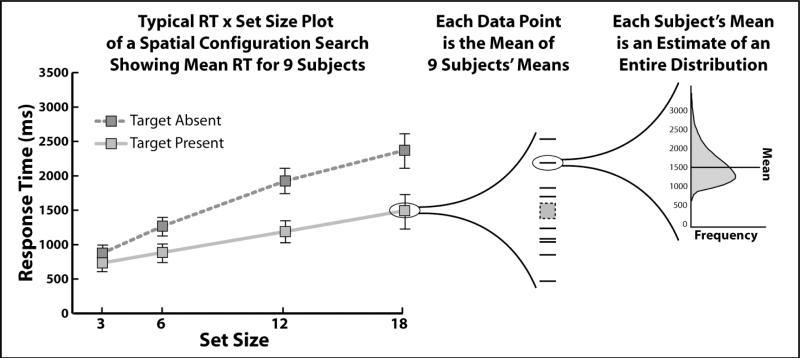
However, the standard RT × set size graph represents only the tip of the metaphorical iceberg (Figure 1, left). Each data point on the graph is the mean of many observers’ average response time (Figure 1, middle). Moreover, an observer's mean or median RT is merely an estimate of the central tendency of an entire underlying RT distribution (Figure 1, right). Those underlying RT distributions have rarely been examined, perhaps because accurately estimating their shapes requires hundreds of trials for each distribution (Van Zandt, 2000).

Figure 1.

Data compression in a standard mean RT × set size plot. Each data point is an abstraction of an entire underlying distribution of RTs. Usually, the RT distribution for each condition and for each subject is not collected because it requires so many trials to estimate it accurately.

Nevertheless, analyzing the full distribution has advantages that make it worth the effort. First, the widespread use of means reflects the implicit assumption of a Gaussian distribution, though it is known that RTs are not normally distributed (Luce, 1986; Van Zandt, 2000). The assumption of normality may have consequences for the treatment of RT data. Consider the common practice of eliminating RTs as outliers based their distance from the mean in terms of standard deviations. Since RT distributions are highly skewed, this procedure has the unintended consequence of truncating the positive tail of the distribution far more than the negative tail (Miller, 1988, 1991; Ulrich & Miller, 1994).

Second, some experimental manipulations affect only part of the RT distribution. For instance, an increase in mean RT could be due to either an increase in skew or a shift in the distribution (Spieler, Balota, & Faust, 2000). Such information is lost in an analysis of means alone. Consequently, many researchers have turned to distributional analyses in order to more precisely characterize cognitive and perceptual phenomena (Bricolo, Gianesini, Fanini, Bundesen, & Chelazzi, 2002; Gottlob, 2004; Heathcote, Popiel, & Mewhort, 1991; Hockley, 1984). For example, Heathcote, et al. (1991) analyzed the RT distributions produced on a Stroop color naming task. They used the Vincentizing method (Ratcliff, 1978) to create group RT distributions, which were then fit with the ex-Gaussian function (convolution of the Gaussian and exponential functions; Burbeck & Luce, 1982). They determined that when participants named the color of a word, the mean of the Gaussian portion of the RT distribution was slowed in the incongruent condition and speeded in the congruent condition, whereas the standard deviation of the Gaussian component was slowed for the incongruent condition but not the neutral or congruent conditions. Furthermore, the exponential portion of the RT distribution increased for both the congruent and incongruent condition relative to the neutral condition. These results are more sophisticated than an analysis of means alone, illustrating the differential effects of the conditions on the mean, standard deviation, and skew of the RT distribution, as interpreted through the ex-Gaussian function (more on this function below).

Most importantly for our purposes, RT distributions might be used to constrain models of visual search. Many models, positing quite different mechanisms, can qualitatively account for the basic patterns of mean RTs (Duncan & Humphreys, 1992; Grossberg, Mingolla, & Ross, 1994; McElree & Carrasco, 1999; Wolfe, 1994; Wolfe, et al., 1989). The challenge to predict RT distributions might winnow the field; in fact, it is our belief that none of the current crop of models successfully captures all the details of RT distributions (Wolfe, Palmer, & Horowitz, 2009).

This paper has two goals. First, we will describe the properties of RT distributions for search tasks spanning a broad range of difficulty. Second, we will consider the implications of these distributions for models of visual search. In particular, we will be focusing on how the parameters of four popular distribution functions are affected by the experimental variables of task, set size, and target presence or absence.

We investigated the empirical RT distributions for three types of visual search: an easy feature search, an intermediate conjunction search, and a more difficult spatial configuration search (all three tasks described below). We gathered 500 trials per condition for 9-10 participants in each task and fit four functions (ex-Gaussian, ex-Wald, Gamma, and Weibull) to each RT distribution using maximum likelihood estimation methods. These distributions were chosen because each has a history in cognitive psychology and parameters that have been associated with specific components of models. The parameters values for the fits are provided in Appendix A and the analyses of the statistical trends in the fits are reported in Appendix B.

EXPERIMENTAL METHODS

The data in this paper come from three visual search tasks that span a range of processing difficulties (Figure 2). In the feature search, the target was a red vertical rectangle among green vertical rectangles. This is a highly efficient search task, typically yielding search slopes near zero. Next, in the conjunction search, observers searched for a red vertical rectangle among green vertical and red horizontal rectangles. This task typically yields RT × set size functions with a moderate slope of around 10 ms/item. Finally, the spatial configuration task required observers to search for a digital 2 among digital 5s; items composed of the same horizontal and vertical components, but in different spatial configurations. This task typically yields inefficient RT × set size slopes between 30 and 60 ms/item. Task, set size, and target presence/absence all influence mean RT and, depending on one's model, might be expected to alter the distribution of RTs as well.

Figure 2.

Illustrations of the three tasks. Actual stimuli were presented on a black background. Filled black rectangles correspond to red, outlined rectangles correspond to green, and the digital 2s and 5s were white. On the left, the target was a red vertical rectangle among green vertical rectangles (feature search). In the middle, the target was a red vertical rectangle among green vertical and red horizontal rectangles (conjunction search). On the right, the target was a digital 2 among digital 5s (spatial configuration search).

We fit the RT data from each condition and subject with four different distributions: ex-Gaussian, ex-Wald, Gamma, and Weibull, chosen because the parameters that determine their shape, spread or placement have been theorized to reflect particular mental representations or processes (e.g. Luce, 1986). Complete details of the stimuli and methods as well as traditional mean RT × set size and error analyses are reported in (Wolfe, et al., 2009).

Brief Description of Methods

We present the data for 28 observers between the ages of 18-55 (only one observer older than 30) who participated in the three tasks. Each observer had normal visual acuity and color perception, gave informed consent, and was paid $8 per hour for participating. We collected approximately 4000 trials per subject in each of three tasks: feature search, conjunction search, and spatial configuration search (Figure 2). For each task, there were four set sizes (3, 6, 12, 18) and targets were present on 50% of trials. Both the set size and presence of a target were determined probabilistically from trial to trial, meaning that some cells have slightly different numbers of trials than others. For each combination of set size and target presence, there were about 500 trials, enough to create meaningful RT distributions.

Data Analysis Procedures

We removed 80 of the nearly 112,000 trials (.07%) from this data set because RTs were < 200 ms or > 4000 ms for the feature and conjunction search tasks and RTs < 200 ms or > 8000 ms in the spatial configuration search task¹. The entire data set (including excluded trials) as well as distribution fitting code is available at http://search.bwh.harvard.edu/new/data_set.html.

The empirical RT distributions for each participant and condition were fit with three-parameter versions of the ex-Gaussian, ex-Wald, Gamma, and Weibull distributions using maximum likelihood estimation procedures. The Gamma and Weibull functions, which are typically two-parameter functions, were specified in a form that included the extra parameter ξ, which shifts the origin of the function along the x-axis without changing the function's shape. The ex-Wald distribution has four parameters, but the σ parameter, which represents the standard deviation of the drift rate in the diffusion process, was set to 1.0. This assumption does not affect the generalizability of the function fits (Schwarz, 2001). Therefore, all four of our fitting functions had three free parameters and were on an equal footing in terms of their ability to fit the data.

Maximum likelihood estimates were obtained by minimizing the negative log likelihood function for each distribution using the Optimization Toolbox routines in Matlab 7.0.4 (particularly the “fminsearchbnd” function), which are based on the Nelder-Mead simplex search algorithm (e.g. Lagarias, Reeds, Wright, & Wright, 1998). A grand total of 896 distribution fits were computed (28 Participants × 4 Set Sizes × 2 Target-Present/Absent × 4 Distributions).

There are a few assumptions and regularity conditions that must be met for maximum likelihood procedures to yield accurate estimates of population parameters (Azzalini, 1996). First, we assumed that the set of RTs we collected from each participant were sampled from independently and identically distributed (IID) random variables from some underlying distribution that we were trying to estimate. This is a common assumption when dealing with RT observations (e.g. Van Zandt, 2002). It should be noted that it is possible that the data violate the IID assumption due to subtle factors like learning or fatigue. We attempted to address these issues by using experienced psychophysical observers and requiring them to take frequent rest breaks during data collection. However, there is no clear way to tell if the IID assumption was violated. In our analyses, we adopted the common assumption that distributions are IID, but the reader may want to keep this caveat in mind. Second, we used estimation functions with parameters that can vary independently and have continuous densities, both of which are requirements for maximum likelihood procedures to be asymptotically unbiased (Azzalini, 1996). Finally, we collected several hundred observations per condition, which greatly improves the stability and reliability of the maximum likelihood procedure (Azzalini, 1996).

We evaluated parameter trends for each three-parameter distribution with four 3 × 2 × 4 (Task × Target-Present/Absent × Set Size) mixed ANOVAs, with task treated as a between-subjects variable. Follow-up ANOVAs were conducted as necessary to interpret main effects and interactions. Goodness of fit for each function was measured using χ², computed for every subject and condition with the best-fitting parameters for each condition (as determined by maximum likelihood estimation). Bins for the χ² analysis were initially set to every 5^th percentile of the empirical data, with the constraint that there had to be more than five predicted observations per bin (Hays, 1994). If there were five or fewer observations, adjacent bins were combined until there were more than five. The χ² scores were entered into a 4 × 3 × 2 × 4 (Function × Task × Target-Present/Absent × Set Size) repeated measures ANOVA, with task treated as a between-subjects variable. Follow-up ANOVAs and planned, two-tailed t-tests were used to compare the fits of different functions. In order to ease presentation of our main findings, ANOVA results for parameter trends and χ² values of the four distributions are presented in Appendix B. Error bars on graphs represent confidence intervals computed from pooled mean squared error values (Masson & Loftus, 2003).

RESULTS AND DISCUSSION

Raw Histogram Plots

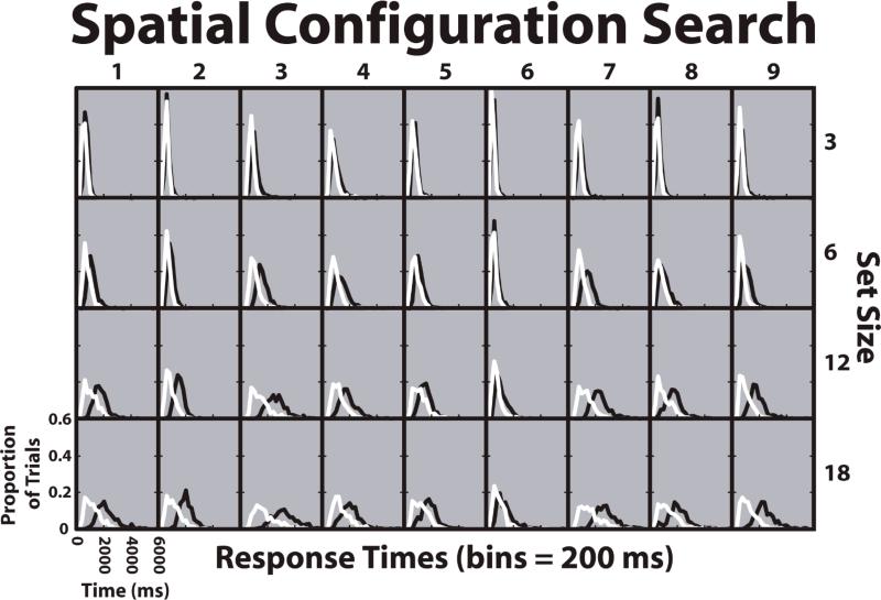
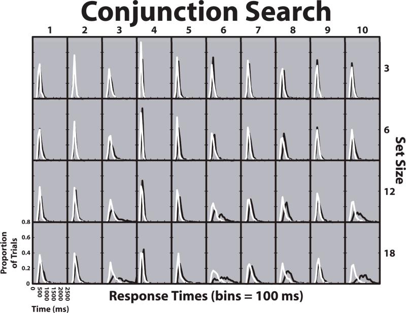
Figures 3-5 show histograms of the RT distributions for each task, display type (target-present or target-absent), set size and participant. The feature, conjunction and spatial configuration histograms were computed with bin sizes of 50, 100, and 200 ms, respectively. Each histogram was normalized so that the total area under each curve was equal to 1.0. The distributions for correct target-present and target-absent trials are displayed in the same graph for comparison.

Figure 3.

Response time histograms for correct trials in the feature search task. Target-present trials are depicted in white and target-absent trials are depicted in black. Axis values are listed in the lower left cell and apply for all plots. The time range in this graph is from 0 to 1000 ms. Each column represents one participant in the task. Each row displays a different set size.

Figure 5.

Response time histograms for correct trials in the spatial configuration search task. Target-present trials are depicted in white and target-absent trials are depicted in black. Axis values are listed in the lower left cell and apply for all plots. The time range in this graph is from 0 to 6000 ms. Each column represents one participant in the task. Each row displays a different set size.

For the feature search task (Figure 3), informal examination of the RT distributions within participant as a function of set size reveal no major differences in shape. Additionally, the shapes of the RT distributions for target-present and target-absent trials remained fairly stable (and similar) for each participant as set size increased. Thus, it appears that the RT distribution data mirror the typical RT × set size data for feature search experiments—changes in set size or target presence or absence did not yield obvious differences in behavior for participants in this kind of search.

Visual inspection of the conjunction search RT distributions plotted in Figure 4 show distributions spreading out slightly at larger set sizes, particularly for target-absent trials. The starting point of the distribution, corresponding to the fastest RTs, appears to remain fairly stable as a function of set size for target-present trials. However, target-absent functions begin slightly later than target-present functions, especially at larger set sizes. Target-absent trials are slightly broader and appear less skewed than target-present trials.

Figure 4.

Response time histograms for correct trials in the conjunction search task. Target-present trials are depicted in white and target-absent trials are depicted in black. Axis values are listed in the lower left cell and apply for all plots. The time range in this graph is from 0 to 2500 ms. Each column represents one participant in the task. Each row displays a different set size.

Informal observation of the RT distribution functions for the spatial configuration search task in Figure 5 suggest clear changes in distribution shape as a function of set size and target presence or absence. Both target-present and target-absent functions appear to spread out more as set size increases, with target-absent functions also shifting to the right. Target-present functions appear to originate from the same starting point regardless of set size.

Four Moments Analyses

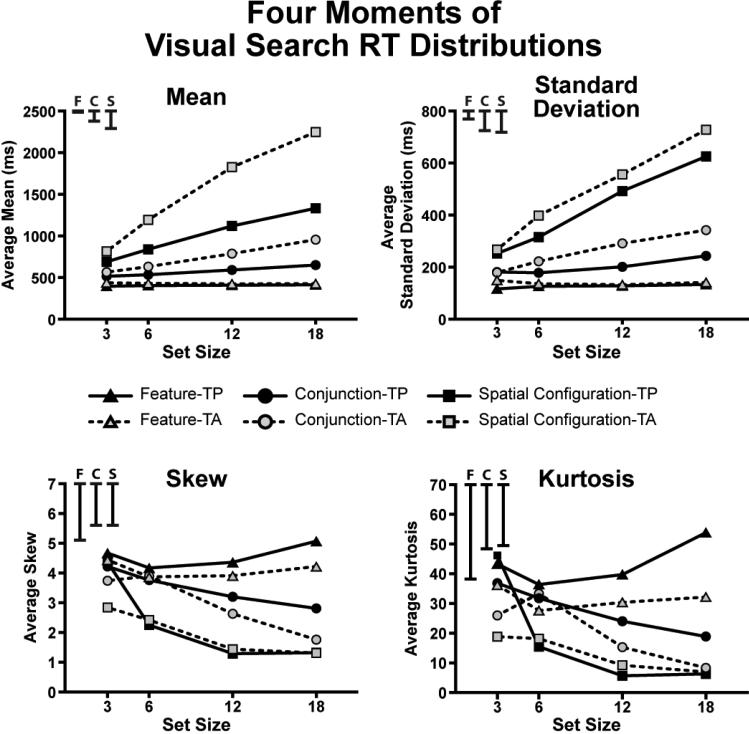
Figure 6 presents the four moments of the RT distributions (mean, standard deviation, skew, and kurtosis) for all tasks and set sizes, averaged across observers. The means and standard deviations of the RTs from this experiment are consistent with those typically observed in the literature (e.g., Cheal & Lyon, 1992; Wolfe, 1998). Perhaps the most surprising trend in this data is that high set size spatial configuration search RT distributions have almost identical skew and kurtosis for both target-present and target-absent distributions despite the fact that the raw histograms look quite different.

Figure 6.

Four moments of visual search response time distributions. Note that standard deviation rather than variance is plotted for the second moment.

Distribution Analysis Results

In this section, we present the average parameter fits for each of four functions: ex-Gaussian, ex-Wald, Gamma, and Weibull. Readers who have found one or the other function useful in other contexts may be interested to see how well the function captures search RT distribution data. More general readers will wish to note whether parameters of a function appear to capture something psychologically real about the search task; e.g. does one parameter track set size? We introduce each function in turn and discuss its applicability to modeling visual search processes.

Ex-Gaussian

This function, named by Burbeck & Luce (1982), is the convolution of a Gaussian and an exponential distribution. The Gaussian portion of the distribution is described by two parameters, mean μ and standard deviation σ. The exponential portion of the ex-Gaussian is captured by the parameter τ, which is related to both the mean and variance of that component. The mean of the ex-Gaussian is μ + τ and the variance is σ² + τ² (Ratcliff, 1978). We used the ex-Gaussian density function defined by Van Zandt (2002) as:

$$f_T(t;\mu ,\sigma ,\tau )=\frac{1}{\tau }\text{exp}\left(-\frac{t}{\tau }+\frac{\mu }{\tau }+\frac{{\sigma }^2}{2{\tau }^2}\right)\Phi \left(\frac{t-\mu -{\sigma }^2∕\tau }{\sigma }\right),$$ (1)

where Φ is the cumulative density function of the standard Gaussian distribution. Since the Gaussian portion of this function has a non-zero density for times less than zero, we constrained the density function so that t ≥ 0.

The components of the ex-Gaussian distribution might correspond to different mental processes. McGill (1963) identified the Gaussian portion of the distribution with decision processes and the exponential portion of the distribution with residual perceptual and response-generation processes. In contrast, Hohle (1965) argued that decision processes might be distributed exponentially, whereas residual processes might be distributed normally. While there is little agreement about which component of the ex-Gaussian distribution corresponds to which hypothetical processing stage (Luce, 1986; Schwarz, 2001), the idea that components of a mixture distribution might reflect particular components of mental processing is appealing (Spieler, et al., 2000). Additionally, the ex-Gaussian distribution is known to fit RTs very well, and so has often been used when examining RT distributions (e.g., Hockley, 1984; Luce, 1986; McElree & Carrasco, 1999; Ratcliff, 1978, 1979; Ratcliff & Murdock, 1976; Spieler, Balota, & Faust, 1996).

Hockley (1984) reported that increases in set size in a visual search task lead to increases in the values of the μ and σ parameters, but not in the τ parameter. That finding is consistent with τ representing the residual motor and neural delays that are theoretically constant across set size in a search (McGill, 1963). Thus, we might expect to observe the same trend in the present data, with τ varying little with set size, while μ and σ increase proportionally. Spieler et al. (2000) noted that parameters in the ex-Gaussian distribution often trade off with one another. In particular, they claimed that the τ parameter is often inversely correlated with the σ parameter. We will also evaluate this claim. Another question of interest is whether the three different visual search tasks will yield three different patterns of parameter trends. It has been argued that the τ parameter is a convenient way to parcel out changes in skew from changes in the mean of an RT distribution (Spieler, et al., 2000), so another question of interest is how the τ parameter correlates with skew.

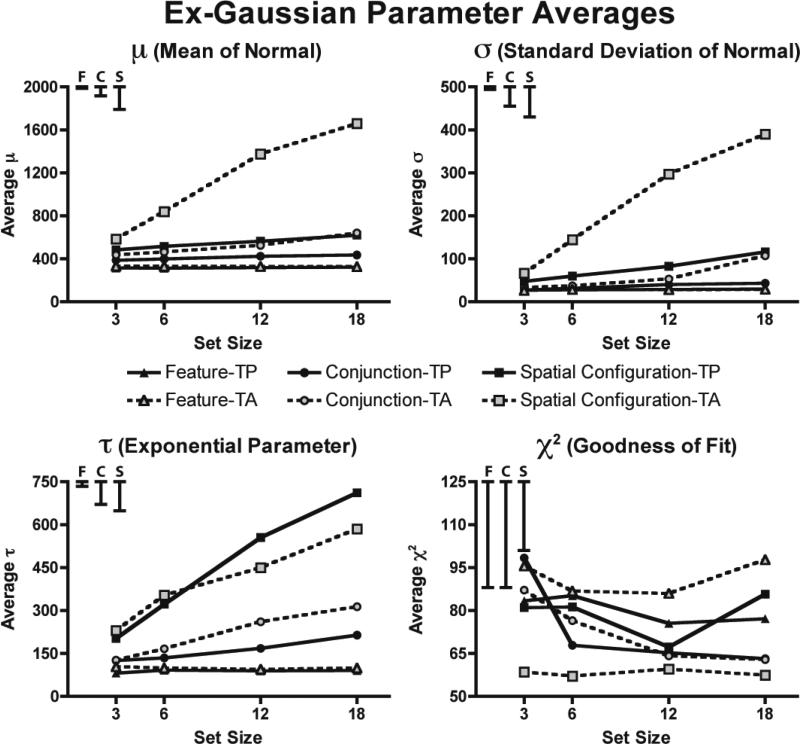
Average parameter values, along with χ² goodness-of-fit measures are plotted in Figure 7. One obvious feature of this graph is that the μ and σ parameters have very similar trends as a function of set size (consistent with observations by Wagenmakers & Brown, 2007), while the τ parameter behaves differently. This observation was supported by the statistical analyses. Omnibus ANOVAs of the μ and σ parameters returned highly significant main effects and interactions for all factors (all p < .0001), whereas omnibus ANOVA of τ parameter trends only detected main effects of task and set size (all p < .0001) and interactions of target presence by task, set size by task, and target presence by set size by task (all p < .005). Neither the main effect of target presence nor the interaction of target presence by set size were significant for the τ parameter (all p > .05, n.s.). Thus, the μ and σ parameter trends were similar to each other, but different than the τ parameter trends.

Figure 7.

Average parameter values for the ex-Gaussian distribution. μ is the mean of the Gaussian component, σ is the standard deviation of the Gaussian component, and τ is the exponential parameter. For the confidence intervals in the upper left, F stands for feature search, C stands for conjunction search, and S stands for spatial configuration search.

Three follow-up ANOVAs on the parameter trends for the feature search task failed to detect any significant main effects or interactions for any of the three parameters (all p > .05, n.s.). Set size and display type do not affect RT distributions in feature search (as indexed by the ex-Gaussian function) any more than they affect means.

For the conjunction search task, analyses of all three ex-Gaussian parameters revealed significant main effects of target presence and set size, as well as significant interactions of target presence by set size (all p < .05). For the spatial configuration search task, all main effects and interactions of μ and σ were highly significant (all p < .0001), whereas for τ, the difference between target-present and target-absent displays failed to reach significance (p > .05, n.s.). The lack of an omnibus main effect of target presence for τ seems to be due to target-absent trials having higher τ values for conjunction search but lower values (on average) for spatial configuration search. These two opposite trends cancelled each other out.

Hockley's (1984) finding that the τ parameter did not change as a function of set size was not replicated in our data set, as evidenced by the significant main effects of set size for the conjunction and spatial configuration search tasks (both p < .0001). Spieler et al.'s (2000) observation that the σ and τ parameters tend to be inversely correlated was also not supported. The overall correlation across the 224 distributions modeled was r = 0.61, t(222) = 11.46, p < .0001. No average correlation for any task was negative.

Finally, we examined the relationship between measurements of skew and the values of the τ parameter. The correlation between these two measurements was negative, r = -0.43, t(222) = -7.02, p < .0001, meaning that higher values of skew were predictive of lower τ values in our data set. Interestingly, both the conjunction and spatial configuration search tasks had negative correlations but the feature search task had a positive correlation between τ and skew.

To evaluate goodness-of-fit, the χ² statistic was computed for every function fit and the scores submitted to an omnibus ANOVA. The analysis detected a significant main effect of task (p < .05) and a reliable interaction of target presence by task (p < .005), but no other trends reached significance (all p > .05, n.s.). χ² values were lowest in the spatial configuration search task (lower χ² indicates better fit), followed by the conjunction and then the feature search tasks. Follow-up one-way ANOVAs for each task failed to find any reliable effects for feature and conjunction search, but did detect a significant main effect of target presence (p < .005) for spatial configuration search. No other trends reached significance (all p > .05, n.s.). The significant main effect of target presence for spatial configuration search, combined with a lack of all other effects, explains the main effect of task and the interaction of target presence by task.

Discussion of ex-Gaussian Fits

The more difficult the search task (and thus, the more extended in time the distribution), the better the fit of the ex-Gaussian to the data. It appears that both the mean (μ) and variance (σ) of the Gaussian component of the ex-Gaussian distribution were similarly modulated by changes in task, set size, and target presence or absence (see also Wagenmakers & Brown, 2007). On the other hand, τ, the exponential component of the ex-Gaussian distribution, showed somewhat different trends than the μ and σ parameters. The analyses found no significant effects (of set size, target presence/absence, or their interaction) in τ for the feature search task, unlike the conjunction and spatial configuration tasks. The effect of target presence on the τ parameter was the opposite for the conjunction and spatial configuration search tasks, with target-absent conjunction displays yielding larger estimates of τ than target-present displays, and target-present spatial configuration displays yielding larger estimates of τ than target-absent displays. But perhaps the most obvious difference in the τ parameter from the μ and σ parameters was that target-present and target-absent trials were similar for the τ parameter in spatial configuration search, but not for the μ and σ parameters.

Ex-Wald

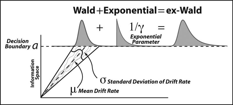
The ex-Wald is the convolution of an exponential and a Wald distribution that attempts to represent both the decision and response components of a response time (Schwarz, 2001) as a diffusion process, a continuous accumulation of information towards some decision threshold (Ratcliff, 1978). The Wald component describes the finishing time distribution of a diffusion processes with a single absorbing boundary. Diffusion models have been successful in modeling response times for a number of cognitive and perceptual tasks (Palmer, Huk, & Shadlen, 2005; Ratcliff, 1978), including visual search (Reeves, Santhi, & Decaro, 2005). Thus, in theory, the Wald portion of the distribution corresponds to the search/decision portion of a RT. The exponential portion of the distribution is intended to capture the residual component of RTs (e.g., motor delays), and is independent of the diffusion process (Schwarz, 2001, 2002).

The scale of the exponential component is described by the parameter γ (actually, 1/γ) which determines both the mean and standard deviation of the exponential. The diffusion process is described by the three parameters of the Wald distribution (Figure 8). The parameter μ represents the mean drift rate of the diffusion process, while σ² represents its variance. The σ parameter is typically set to 1.0 without any loss of generality (Schwarz, 2001). The height of the absorbing boundary is described by the parameter a. We implemented the Schwarz (2001) definition of the ex-Wald, which has the probability density function h defined as:

$$h(t\mid \mu ,\sigma ,a,\gamma )=\gamma \text{exp}\left(-\gamma t+\frac{a(\mu -k)}{{\sigma }^2}\right)\cdot F(t\mid k,\sigma ,a)$$ (2)

where k is defined as:

$$k=\sqrt{{\mu }^2-2\gamma {\sigma }^2}\ge 0$$ (3)

and the cumulative density function of the Wald distribution, F, is defined as:

$$F(w\mid \mu ,\sigma ,a)=\Phi \left(\frac{\mu w-a}{\sigma \sqrt{w}}\right)+\text{exp}\left(\frac{2a\mu }{{\sigma }^2}\right)\cdot \Phi \left(-\frac{\mu w+a}{\sigma \sqrt{w}}\right)$$ (4)

where Φ is the standard cumulative Gaussian function.

Figure 8.

The ex-Wald distribution is the combination of the Wald distribution and the Exponential distribution. The Wald component models the finishing time distribution of a diffusion process in which information accumulates over time towards an absorbing decision boundary. The exponential component is intended to capture residual processes, such as motor response times.

One of the strengths of the ex-Wald function is that it has well-specified theoretical connections to models of process (Heathcote, 2004; Schwarz, 2001), such as the diffusion model (Ratcliff, 1978). These connections can allow one to make reasonable hypotheses about parameter trends as a function of condition (Schwarz, 2001). For instance, as the difficulty of the search task increases from feature search to conjunction to spatial configuration search, we can expect the rate of accumulation of information over time (μ) to decrease. Likewise, increasing set size should cause a decrease in μ, since large set size displays contain more information to process than small set size displays.

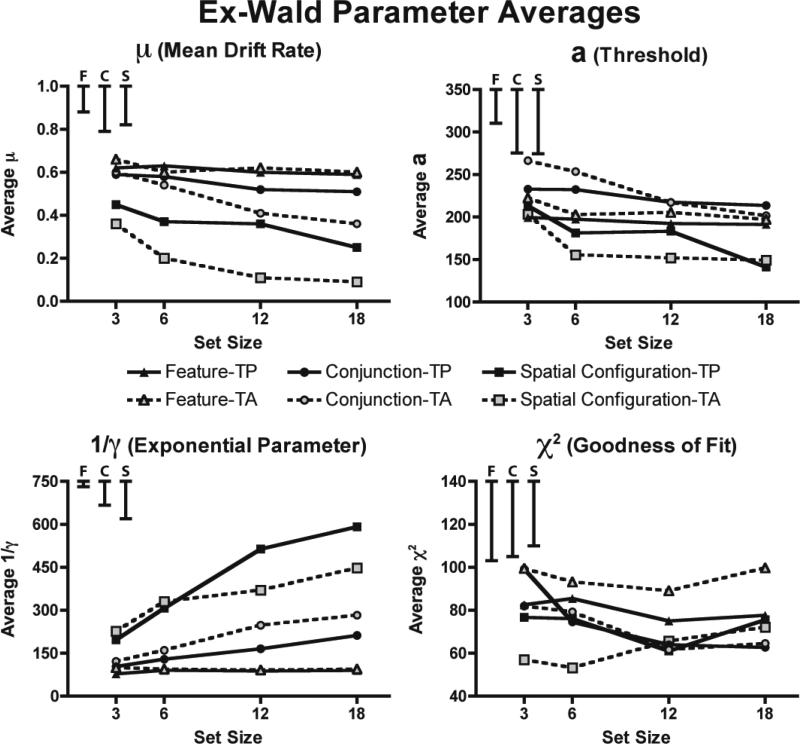
According to our maximum likelihood estimates, the μ parameter decreased with task difficulty and set size, as predicted (Figure 9). Analyses of the μ parameter trends showed main effects of task, target presence and set size (all p < .01). The only interaction was target presence by task (p < .05; all others p > .05). This interaction reflected the fact that the drift rate was reduced for target absent trials in the spatial configuration search task (p < .05), while target presence or absence had no effect on drift rate for the other search tasks (all p > .05).

Figure 9.

Average parameter values for the ex-Wald distribution. μ is the mean drift rate, σ, the standard deviation of the drift rate was set to 1, a the level of the absorbing boundary, and 1/γ is the exponential parameter. For the confidence intervals in the upper left, F stands for feature search, C stands for conjunction search, and S stands for spatial configuration search.

The average estimated level of the absorbing boundary, a, was higher for the conjunction search task than for the feature search task, but the spatial configuration search task had the lowest values overall. The combination of slower information accumulation and lower decision thresholds reflects the typical speed-accuracy covariance across tasks. ANOVAs on the estimated a parameter returned main effects of task and set size (both p < .05), but no other significant findings (all p > .05). T-tests on the three tasks showed that the average level of the absorbing boundary a for the conjunction search and spatial configuration search tasks differed reliably, t(8) = 3.60, p < .01, but no other comparison was significant (all p > .05). Follow-up ANOVAs on each of the three tasks revealed no significant trends in either the feature or conjunction search data (all p > .05), but a reliable main effect of set size for the spatial configuration search data (p < .05).

Analyses of the exponential parameter 1/γ detected main effects of task and set size, as well as interactions of target presence by task, set size by task, and the three-way interaction of target presence by set size by task (all p < .005). No other trends in the omnibus ANOVA for 1/γ reached significance (all p > .10). Follow up ANOVAs on the individual tasks found no significant effects for feature search (all p > .05), but detected main effects of target presence and set size for conjunction search (both p < .05) and a main effect of set size and an interaction of target presence by set size for the spatial configuration search task (both p < .05). For the conjunction search task, values of 1/γ increased significantly with set size, with target-absent trials for conjunction search consistently yielding higher values of 1/γ than target-present trials. Spatial configuration search, on the other hand, had larger values of 1/γ for target-present trials, but only for the two highest set sizes. The trends of the estimated exponential parameter 1/γ for the ex-Wald distribution are highly similar to the estimated exponential parameter τ in the ex-Gaussian distribution, as comparison of the lower-left panels of Figures 7 and 9 will confirm.

Omnibus ANOVA of the χ² goodness-of-fit measure detected a main effect of task and a significant interaction of target presence by task (both p < .05). Spatial configuration search data were better fit by the ex-Wald distribution than were feature search data, t(8) = 2.71, p = .027, though the other comparisons were not significant (all p > .10).

Discussion of ex-Wald Fits

More difficult search tasks lead to lower estimates of μ, indicating that information about more difficult displays accumulated more slowly than did information about easier displays. The μ parameter appears to be inversely proportional to mean RT. The 1/γ parameter also showed a pattern of data that was qualitatively similar to the mean RT data, with higher estimates of the exponential parameter for difficult spatial configuration searches than for moderate conjunction searches or easy feature searches. Both the μ and 1/γ parameters showed the same qualitative ordering of values as would be expected based on search difficulty.

The threshold parameter a, on the other hand, did not yield estimated values that had a clear ordered correspondence with task difficulty. Spatial configuration search had the lowest values of a, followed by feature search and then conjunction search. Lower levels of a indicate lower thresholds for responding, which lead to shorter RTs and more errors, though these trends will be modulated by the drift rate, μ. Starting with feature search, neither μ, nor a, nor 1/γ varied much as a function of set size or target presence or absence. For target-present conjunction searches, the drift rates had values similar to feature search, while the thresholds were higher. Conversely, for spatial configuration searches, the drift rate is so slow that even with a very low decision boundary, RTs remain much higher than for the other tasks.

According to the ex-Wald model, mean RT differences between conditions are a combination of factors including perceptual difficulty (i.e., drift rate μ) and the observer's internal criteria (i.e., threshold a), as opposed to simply reflecting difficulty, as is implicit in other models. Through the threshold parameter a, the ex-Wald acknowledges the contribution of error rates to understanding search behavior. All other things being equal, lower values of a should yield faster RTs but higher error rates. Of course, all other things are not equal across tasks, so we cannot make direct inferences about what the error rates should be. A theory relating RT and accuracy in search is beyond the scope of the this paper, but the interested reader can look at (Palmer, et al., 2005) for an approach using the diffusion model, and to (Wolfe, et al., 2009) for an analysis of the error rates from this dataset.

Gamma

This function is defined as the sum of a series of exponential processes. Each exponential process may have a different scale, but the average scale of the processes is captured by the parameter α. The shape parameter β reflects the approximate number of exponentials contributing to the function. The shift parameter ξ moves the function along the x-axis without affecting its shape. The density function of the shifted Gamma distribution (Dolan, van der Maas, & Molenaar, 2002) is:

$$f(x\mid \alpha ,\beta ,\xi )=\frac{{(x-\xi )}^{\beta -1}\text{exp}\left(-\frac{x-\xi }{\alpha }\right)}{{\alpha }^{\beta }\Gamma \left(\beta \right)}$$ (5)

where Γ(β) is the gamma function.

Consider two accounts of the β parameter. In one version of a serial model, each deployment of attention might add an exponentially distributed increment to the RT and β would increase with set size. Alternatively, β might reflect a number of larger stages (e.g. initial processing, search, & decision). In this case, β would be relatively constant across set size and, perhaps, across tasks.

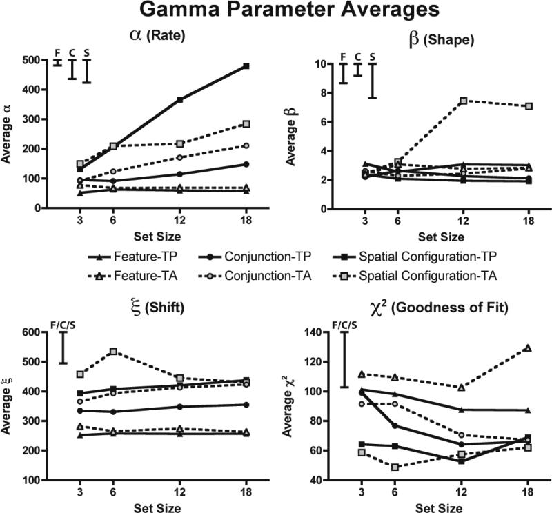
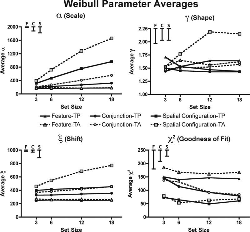
Figure 10 presents the average parameters from the fitted gamma distributions. It is clear that β varied little with set size or task. Except for the higher set sizes of target absent, spatial configuration, the data can be modeled as representing the contributions of 2-3 exponentials with the differences between the conditions captured by the rate parameter α which increased with set size for the spatial configuration and conjunction tasks (both p < .0005), but not the feature task (p > .05). Rates were overall slower for more difficult tasks (p < .0001). No individual task yielded a significant main effect of set size for β (all p > .05), though the omnibus main effect of set size reached significance (p < .005).

Figure 10.

Average parameter values for the Gamma distribution. α is the rate parameter, β is the shape parameter, and ξ is the starting time parameter. For the confidence intervals in the upper left, F stands for feature search, C stands for conjunction search, and S stands for spatial configuration search.

The shift parameter ξ was stable across set size (p > .05) but varied as a function of task (p < .0001) and target presence (p < .01). Unsurprisingly, increasing task difficulty shifted the RT distributions later in time.

Analysis of the χ² goodness-of-fit measure revealed a main effect of task (p < .0005), but no other significant main effects or interactions (all p > .05). Overall, the gamma function appeared to be somewhat better-suited for describing behavior in the spatial configuration search task than either the feature or conjunction search tasks.

Discussion of Gamma Parameter Fits

The number of exponentials making up the gamma function, β, did not track set size, arguing against modeling even inefficient search as a series of exponentially-distributed attentional shifts. This finding should not be taken as evidence either way regarding serial attentional shifts in search, only against one possible implementation of a serial model. The gamma parameter fits are more consistent with a model that sees RT distributions as composed of 2-3 exponentially distributed processes: e.g. initial feed-forward processing, the search process, and response selection/execution. In this account, α, increasing with RT, captures the duration of search processes while ξ – which varied with task and target-present vs. target-absent, but not set size – would seem to be more closely tied to decision processes.

This account broadly describes the parameter fits except for the target absent RTs for the larger set sizes of the spatial configuration task. Here the β parameter suddenly grows suggesting that some different factor is contributing to the RT distributions in these for the longest target-absent searches.

Weibull

For random variables such as RT that are bounded by zero at the lower end and can extend to infinity at the upper end, like a series of races, the asymptotic description of their minima (i.e., the “first place” finishing times) is well captured by a Weibull function (Logan, 1992). The version of the Weibull used in our analyses has three parameters: the shape parameter γ, the scale parameter α, and the shift parameter ξ. We used the form of the Weibull defined by Johnson, et al. (1994), as reported in Dolan, et al. (2002):

$$f(x\mid \alpha ,\gamma ,\xi )=\frac{\gamma }{\alpha }{\left(\frac{x-\xi }{\alpha }\right)}^{\gamma -1}\text{exp}\left(-{\left[\frac{x-\xi }{\alpha }\right]}^{\gamma }\right)$$ (7)

When the shape parameter γ = 1, the Weibull distribution is equal to an exponential distribution (Chechile, 2003). When γ = 3.6, the Weibull is approximately normal (Logan, 1992). Since most RT distributions are positively skewed but not normal, we can expect γ to take on a value somewhere between 1 and 3.6.

Weibull distributions have been used to model RTs in a variety of cognitive tasks (Rouder, Lu, Speckman, Sun, & Jiang, 2005), particularly those which can be modeled as a race among competing units (Cousineau, Goodman, & Shiffrin, 2002). While Logan (1992) successfully used the Weibull to explain memory search RTs, to our knowledge there has been no systematic exploration of its applicability to visual search.

Discussion of Weibull Parameter Fits

The α parameter of the Weibull function appears to share the same qualitative trends as the mean RT data, with all main effects and interactions being highly significant (all p < .0001). This parameter showed a pattern of values more similar to the mean RT data than any other parameter in the four functions we examined.

Examining the upper right panel of Figure 11, it is interesting to note the similarity to the fits of the gamma distribution. Here, the γ parameter changes very little with set size or target presence except for the target absent trials at the larger set sizes for spatial configuration search. Consistent with these observations, analyses of the γ trends detected no main effect of task (p > .10), but there were reliable main effects of target presence and set size, as well as significant interactions between those factors along with a three-way interaction of target presence by set size by task (all p < .01). γ did not significantly differ as a function of set size for feature or conjunction search displays (all p > .10), but γ values were reliably larger for target absent spatial configuration search, as evidenced by an interaction of target presence by set size (all p < .0005) for that search task.

Figure 11.

Average parameter values of the Weibull function. α is the scale parameter, γ is the shape parameter, and ξ is the starting time parameter. For the confidence intervals in the upper left, F stands for feature search, C stands for conjunction search, and S stands for spatial configuration search.

Like the α parameter, the omnibus analysis of the ξ parameter revealed trends similar to the mean RT data. That is, as set size increased, the starting position of the best-fitting Weibull function also increased, with target-absent trials showing a more rapid increase as a function of set size than target-present trials. The main effects of task, target presence and set size, as well as all interactions between those factors being highly significant (all p < .0001).

The Weibull function only seemed to provide a consistently good fit to the data for the spatial configuration search task. Omnibus ANOVA of the χ² goodness-of-fit metric revealed main effects of task and set size, as well as an interaction of task by set size (each p < .01). The Weibull function fit spatial configuration search distributions better than conjunction search, which were in turn better fit by the Weibull than the feature search data (both p < .01). Additionally, higher set size displays in the conjunction search and spatial configuration search tasks were more closely fit by the Weibull than lower set size displays (all p < .05).

DISCUSSION

Comparing Function Fits

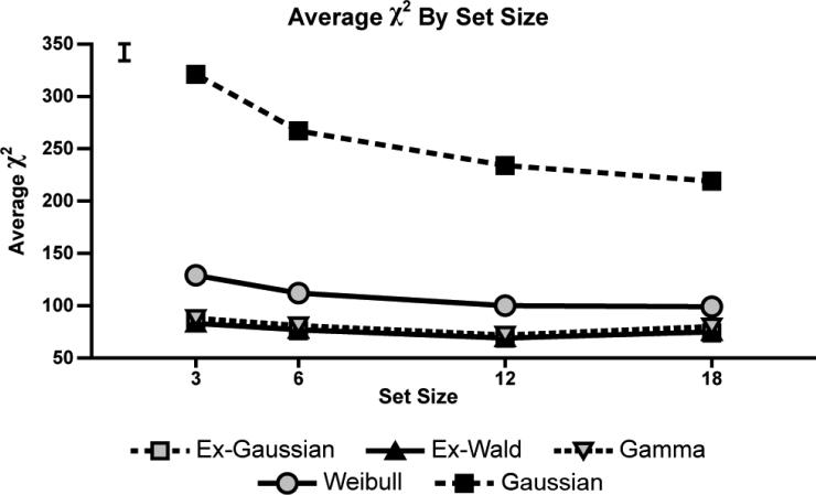
How impressed should one be by the fits of these functions to the data and by the differences between the fits of the functions? Can this approach be used to reject hypotheses about the RT distributions? Figure 12 shows the χ² error as a function of set size, averaged over task and target presence/absence. For comparison, we add the error obtained by fitting a standard Gaussian function to the data, since a simple Gaussian is the implicit assumption of the standard practice of reporting mean and standard errors of RT data. Fortunately, our chosen functions fit the data substantially better than the Gaussian. Furthermore, not all plausible functions are equally good at fitting the data. In particular, the Weibull fits were systematically worse than the fits for the other three functions.

Figure 12.

Average χ² score as a function of set size for the four distributions with added data from the fit of a Gaussian function. Lower scores indicate better fit. Error bar represents standard error of the mean.

To assess these impressions, we submitted the χ² goodness of fit values to a 4 × 3 × 2 × 4 (Function × Task × Target Presence × Set Size) mixed ANOVA with task treated as a between-subjects variable (omitting the Gaussian data). We observed a main effect of function type, and t-tests of the overall function fits showed that the Weibull function was worse than the other three functions (all p < .0001). The ex-Gaussian function yielded the closest fit to the data, overall, followed by the ex-Wald, Gamma and then the Weibull function, though there is little difference between the performance of the first three functions. The close ties of the ex-Wald distribution to diffusion process models makes this function particularly relevant to search, with a clear set of interpretations for its parameters (e.g. Ratcliff, 1978; Schwarz, 2001). The ex-Gaussian function also fits these and other RT distributions well (Hohle, 1965) and the theoretical status of the individual parameters in the ex-Gaussian has been well-explored by many researchers (Hockley, 1984; Luce, 1986; Ratcliff, 1978; Ratcliff & Murdock, 1976; Spieler, et al., 1996). However, the ex-Gaussian parameters are not as strongly tied to computational models of search as the ex-Wald parameters.

Similarities Among Parameter Trends

One unique opportunity provided by the current analyses of visual search RT distribution data is the ability for us to examine similarities in parameter trends across the four fitting functions. We have identified three patterns of parameter values that appear in two or more functions, indicating that the different fitting functions might be picking up similar trends in the RT distribution data.

Parameter Trend #1

Similar exponential parameter trends for all conditions as a function of set size for three of the four fitting functions. Three functions include an exponential component scale parameter (τ in the ex-Gaussian, 1/γ in the ex-Wald, and the exponential scale parameter α in the Gamma). The parameter values look similar in all cases and qualitatively mirror the mean RT data. The only place where they all depart from the pattern of the mean RT data is for the higher set sizes of the target absent trials of the spatial configuration search. Here the parameter values are lower than the values for target present. It is interesting that these conditions also produce the highest error rates (Wolfe, et al., 2009).

Parameter Trend #2

The β parameter for the Gamma function and γ for the Weibull function respond to the shape of the distributions. These show marked elevation for the same higher set sizes of target absent trials in spatial configuration search. The shape parameters are otherwise quite constant. Higher values for the shape parameters of both the Gamma and Weibull functions yield distributions that are less positively skewed than lower values. The fact that the conditions with high shape parameter values also have high miss error rates (Wolfe, et al., 2009) suggests that observers may have abandoned their searches too early, which would lower skew of correct target absent distributions since long RTs in the tails would be more rare.

Parameter Trend #3

Finally, several functions have a parameter or parameters that scale linearly with set size for the target absent trials of the spatial configuration search while the same parameter remains relatively flat in contrast for other conditions. These are parameters that capture the rightward shift and spread of the target absent data. In the ex-Gaussian function, both μ and σ increased rapidly for spatial configuration target-absent distributions compared to all other conditions. For the ex-Wald function, the quantity 1/μ (indicating drift time of the diffusion process rather than drift rate μ presented earlier) increases more dramatically for target-absent spatial configuration searches than for the other conditions, mirroring the trends in the other parameters. Finally, the shift parameter ξ for the Weibull function exhibits the same pattern, increasing almost six times as much in the spatial configuration target-absent vs. target-present distributions.

Exponential Processes in Visual Search

Perhaps the most interesting feature of the distribution analyses is that the three functions with an exponential component were all more successful at modeling RT distributions than the one function (the Weibull) without an exponential component. Furthermore, these exponential factors qualitatively capture the basic pattern of mean RTs. As noted in the previous section, the exponential parameter trends for the ex-Gaussian, ex-Wald, and Gamma functions are all very similar. One interpretation in the literature is that these exponential components reflect residual (non-decision) processes in the generation of response times (McGill, 1963; Schwarz, 2001). However, in the visual search tasks explored here, these components seem to reflect something more like the search process itself (Hohle, 1965). It is worth noting that an “amnesic” serial search mechanism would produce exponentially distributed search times. An amnesic search is one in which rejected distractors are not marked or inhibited, i.e., sampling with replacement. There is some evidence in favor of amnesic search (Horowitz & Wolfe, 1998, 2005), though the topic is controversial (Dukewich & Klein, 2005; Shore & Klein, 2000).

Either these exponential parameters, often linked to residual processing, don't correspond to residual processing at all, or “residual” processes actually play a significant role in shaping the pattern of RTs in search tasks. Perhaps, to borrow an analogy from the field of biology, these residual processes that we had long regarded as “junk DNA” are actually encoding something important. We suspect that this may be the case, but more work needs to be done before any strong conclusions can be drawn.

CONCLUSIONS

The purpose of this project was to move beyond analysis of mean RT in visual search by trying to capture the full RT distributions. We acquired approximately 500 trials per cell from three different benchmark visual search tasks: feature search, conjunction search, and spatial configuration search. We then evaluated the ability of four popular functions to capture the resulting empirical RT distributions. The ex-Gaussian, ex-Wald, and Gamma functions all provided good fits to the empirical data, while the Weibull function did not perform as well. Interestingly, several of the functions had similar parameter trends. Most notably, the three best-fitting functions had exponential components that responded in similar ways to variations in task and set size. Given that many theories of visual search can easily reproduce mean RT data, we hope that the fuller analyses of RT distributions presented here will aid theorists in testing and developing models of visual search.

References

- Azzalini A. Statistical inference based on likelihood. CRC Press; Boca Raton: 1996. [Google Scholar]
- Bricolo E, Gianesini T, Fanini A, Bundesen C, Chelazzi L. Serial attention mechanisms in visual search: a direct behavioral demonstration. Journal of Cognitive Neuroscience. 2002;14(7):980–993. doi: 10.1162/089892902320474454. [DOI] [PubMed] [Google Scholar]
- Burbeck SL, Luce RD. Evidence from auditory simple reaction times for both change and level detectors. Perception & Psychophysics. 1982;32(2):117–133. doi: 10.3758/bf03204271. [DOI] [PubMed] [Google Scholar]
- Cheal M, Lyon DR. Attention in visual search: Multiple search classes. Perception & Psychophysics. 1992;52(2):113–138. doi: 10.3758/bf03206765. [DOI] [PubMed] [Google Scholar]
- Chechile RA. Mathematical tools for hazard function analysis. Journal of Mathematical Psychology. 2003;47:478–494. [Google Scholar]
- Chelazzi L. Serial attention mechanisms in visual search: a critical look at the evidence. Psychological Research. 1999;62(2-3):195–219. doi: 10.1007/s004260050051. [DOI] [PubMed] [Google Scholar]
- Chun MM, Wolfe JM. Visual Attention. In: Goldstein EB, editor. Blackwell's Handbook of Perception. Blackwell; Oxford, UK: 2001. pp. 272–310. Ch 9. [Google Scholar]
- Cousineau D, Goodman V, Shiffrin R. Extending statistics of extremes to distributions varying in position and scale and the implications for race models. Journal of Mathematical Psychology. 2002;46:431–454. [Google Scholar]
- Dolan CV, van der Maas HL, Molenaar PC. A framework for ML estimation of parameters of (mixtures of) common reaction time distributions given optional truncation or censoring. Behavioral Research Methods, Instruments & Computers. 2002;34(3):304–323. doi: 10.3758/bf03195458. [DOI] [PubMed] [Google Scholar]
- Driver J, Vuilleumier P. Perceptual awareness and its loss in unilateral neglect and extinction. Cognition. 2001;79(1-2):39–88. doi: 10.1016/s0010-0277(00)00124-4. [DOI] [PubMed] [Google Scholar]
- Dukewich KR, Klein RM. Implication of search accuracy for serial self-terminating models of search. Visual Cognition. 2005;12(7):1386–1403. [Google Scholar]
- Duncan J, Humphreys GW. Visual search and stimulus similarity. Psychological Review. 1989;96(3):433–458. doi: 10.1037/0033-295x.96.3.433. [DOI] [PubMed] [Google Scholar]
- Duncan J, Humphreys GW. Beyond the search surface: visual search and attentional engagement. Journal of Experimental Psychology: Human Perception and Performance. 1992;18(2):578–588. doi: 10.1037//0096-1523.18.2.578. discussion 589-593. [DOI] [PubMed] [Google Scholar]
- Gottlob LR. Location cuing and response time distributions in visual attention. Perception & Psychophysics. 2004;66(8):1293–1302. doi: 10.3758/bf03194999. [DOI] [PubMed] [Google Scholar]
- Grossberg S, Mingolla E, Ross WD. A neural theory of attentive visual search: interactions of boundary, surface, spatial, and object representations. Psychological Review. 1994;101(3):470–489. doi: 10.1037/0033-295x.101.3.470. [DOI] [PubMed] [Google Scholar]
- Hays WL. Statistics. Harcourt Brace College Publishers; New York: 1994. [Google Scholar]
- Heathcote A. Fitting wald and ex-Wald distributions to response time data: an example using functions for the S-PLUS package. Behavioral Research Methods, Instruments & Computers. 2004;36(4):678–694. doi: 10.3758/bf03206550. [DOI] [PubMed] [Google Scholar]
- Heathcote A, Popiel SJ, Mewhort DJ. Analysis of response time distributions: An example using the stroop task. Psychological Bulletin. 1991;109(2):340–347. [Google Scholar]
- Hockley WE. Analysis of response time distributions in the study of cognitive processes. Journal of Experimental Psychology: Learning, Memory, and Cognition. 1984;6:598–615. [Google Scholar]
- Hohle RH. Inferred Components of Reaction Times as Functions of Foreperiod Duration. Journal of Experimental Psychology. 1965;69:382–386. doi: 10.1037/h0021740. [DOI] [PubMed] [Google Scholar]
- Horowitz TS, Wolfe JM. Visual search has no memory. Nature. 1998;394(6693):575–577. doi: 10.1038/29068. [DOI] [PubMed] [Google Scholar]
- Horowitz TS, Wolfe JM. Visual search: The role of memory for rejected distractors. In: Itti L, Rees G, Tsotsos JK, editors. Neurobiology of Attention. Elsevier; San Diego: 2005. pp. 264–268. [Google Scholar]
- Johnson NL, Kiotz S, Balakrishnan N. Continuous univariate distributions. 2nd ed. Vol. 1. Wiley; New York: 1994. [Google Scholar]
- Lagarias J, Reeds J, Wright M, Wright P. Convergence properties of the Nelder-Mead simplex method in low dimensions. SIAM Journal of Optimization. 1998;9(1):112–147. [Google Scholar]
- Logan GD. Shapes of reaction-time distributions and shapes of learning curves: A test of the instance theory of automaticity. Journal of Experimental Psychology: Learning, Memory, and Cognition. 1992;18(5):883–914. doi: 10.1037//0278-7393.18.5.883. [DOI] [PubMed] [Google Scholar]
- Luce RD. Response times: Their role in inferring elementary mental organization. Oxford University Press; New York: 1986. [Google Scholar]
- Luck SJ, Vecera SP. Attention. In: Pashler H, Yantis S, editors. Stevens’ Handbook of Experimental Psychology. 3rd ed. Vol. 1. Wiley and Sons; New York: 2002. pp. 235–286. Sensation and Perception. [Google Scholar]
- Masson ME, Loftus GR. Using confidence intervals for graphically based data interpretation. Canadian Journal of Experimental Psychology. 2003;57(3):203–220. doi: 10.1037/h0087426. [DOI] [PubMed] [Google Scholar]
- McElree B, Carrasco M. The temporal dynamics of visual search: evidence for parallel processing in feature and conjunction searches. Journal of Experimental Psychology: Human Perception & Performance. 1999;25(6):1517–1539. doi: 10.1037//0096-1523.25.6.1517. [DOI] [PMC free article] [PubMed] [Google Scholar]
- McGill WJ. Stochastic latency mechanisms. In: Luce RD, Bush RR, Galanter E, editors. Handbook of Mathematical Psychology. Vol. 1. Wiley; New York: 1963. pp. 309–360. [Google Scholar]
- Miller J. A warning about median reaction time. Journal of Experimental Psychology: Human Perception & Performance. 1988;14(3):539–543. doi: 10.1037//0096-1523.14.3.539. [DOI] [PubMed] [Google Scholar]
- Miller J. Reaction time analysis with outlier exclusion: bias varies with sample size. Quarterly Journal of Experimental Psychology A. 1991;43(4):907–912. doi: 10.1080/14640749108400962. [DOI] [PubMed] [Google Scholar]
- Palmer J, Huk AC, Shadlen MN. The effect of stimulus strength on the speed and accuracy of a perceptual decision. Journal of Vision. 2005;5(5):376–404. doi: 10.1167/5.5.1. [DOI] [PubMed] [Google Scholar]
- Pashler H. The Psychology of Attention. MIT Press; Cambridge, MA: 1998. [Google Scholar]
- Ratcliff R. A Theory of Memory Retrieval. Psychological Review. 1978;85:59–108. [Google Scholar]
- Ratcliff R. Group reaction time distributions and an analysis of distribution statistics. Psychological Bulletin. 1979;86(3):446–461. [PubMed] [Google Scholar]
- Ratcliff R, Murdock B. Retrieval processes in recognition memory. Psychological Review. 1976;86:190–214. [Google Scholar]
- Reeves A, Santhi N, Decaro S. A random-ray model for speed and accuracy in perceptual experiments. Spatial Vision. 2005;18(1):73–83. doi: 10.1163/1568568052801582. [DOI] [PubMed] [Google Scholar]
- Rouder JN, Lu J, Speckman PL, Sun D, Jiang Y. A hierarchical model for estimating response time distributions. Psychonomic Bulletin & Review. 2005;12(2):195–223. doi: 10.3758/bf03257252. [DOI] [PubMed] [Google Scholar]
- Schwarz W. The ex-Wald distribution as a descriptive model of response times. Behavioral Research Methods, Instruments & Computers. 2001;33(4):457–469. doi: 10.3758/bf03195403. [DOI] [PubMed] [Google Scholar]
- Schwarz W. On the convolution of inverse gaussian and exponential random variables. Communications in Statistics: Theory and Methods. 2002;31(12):2113–2121. [Google Scholar]
- Shore DI, Klein RM. On the manifestations of memory in visual search. Spatial Vision. 2000;14(1):59–75. doi: 10.1163/156856801741369. [DOI] [PubMed] [Google Scholar]
- Spieler DH, Balota DA, Faust ME. Stroop performance in healthy younger and older adults and in individuals with dementia of the Alzheimer's type. Journal of Experimental Psychology: Human Perception & Performance. 1996;22(2):461–479. doi: 10.1037//0096-1523.22.2.461. [DOI] [PubMed] [Google Scholar]
- Spieler DH, Balota DA, Faust ME. Levels of selective attention revealed through analyses of response time distributions. Journal of Experimental Psychology: Human Perception & Performance. 2000;26(2):506–526. doi: 10.1037//0096-1523.26.2.506. [DOI] [PubMed] [Google Scholar]
- Treisman A, Gelade G. A feature-integration theory of attention. Cognitive Psychology. 1980;12(1):97–136. doi: 10.1016/0010-0285(80)90005-5. [DOI] [PubMed] [Google Scholar]
- Treisman A, Gormican S. Feature analysis in early vision: Evidence from search asymmetries. Psychological Review. 1988;95(1):15–48. doi: 10.1037/0033-295x.95.1.15. [DOI] [PubMed] [Google Scholar]
- Treisman A, Sato S. Conjunction search revisited. Journal of Experimental Psychology: Human Perception & Performance. 1990;16(3):459–478. doi: 10.1037//0096-1523.16.3.459. [DOI] [PubMed] [Google Scholar]
- Ulrich R, Miller J. Effects of truncation on reaction time analysis. Journal of Experimental Psychology: General. 1994;123(1):34–80. doi: 10.1037//0096-3445.123.1.34. [DOI] [PubMed] [Google Scholar]
- Van Zandt T. How to fit a response time distribution. Psychonomic Bulletin & Review. 2000;7(3):424–465. doi: 10.3758/bf03214357. [DOI] [PubMed] [Google Scholar]
- Van Zandt T. Analysis of response time distributions. In: Pashler H, Wixted J, editors. Steven's Handbook of Experimental Psychology. 3rd Ed. Vol. 4. John Wiley & Sons, Inc.; New York: 2002. pp. 461–516. [Google Scholar]
- Wagenmakers EJ, Brown S. On the linear relation between the mean and the standard deviation of a response time distribution. Psychological Review. 2007;114(3):830–841. doi: 10.1037/0033-295X.114.3.830. [DOI] [PubMed] [Google Scholar]
- Wolfe JM. Guided Search 2.0: A revised model of visual search. Psychonomic Bulletin & Review. 1994;1(2):202–238. doi: 10.3758/BF03200774. [DOI] [PubMed] [Google Scholar]
- Wolfe JM. What can 1 million trials tell us about visual search? Psychological Science. 1998;9(1):33–39. [Google Scholar]
- Wolfe JM, Cave KR. The psychophysical evidence for a binding problem in human vision. Neuron. 1999;24(1):11–17. doi: 10.1016/s0896-6273(00)80818-1. [DOI] [PubMed] [Google Scholar]
- Wolfe JM, Cave KR, Franzel SL. Guided search: an alternative to the feature integration model for visual search. Journal of Experimental Psychology: Human Perception & Performance. 1989;15(3):419–433. doi: 10.1037//0096-1523.15.3.419. [DOI] [PubMed] [Google Scholar]
- Wolfe JM, Palmer EM, Horowitz TS. Reaction time distributions constrain models of visual search. Vision Research. 2009 doi: 10.1016/j.visres.2009.11.002. submitted. [DOI] [PMC free article] [PubMed] [Google Scholar]
Associated Data
This section collects any data citations, data availability statements, or supplementary materials included in this article.