Assessing and Compensating for Zero-lag Correlation Effects in Time-lagged Granger Causality Analysis of fMRI

Abstract

Effective connectivity in brain networks can be studied using Granger causality analysis which is based on temporal precedence, while functional connectivity is usually derived using zero-lag correlation. Due to the smoothing of the neuronal activity by the hemodynamic response inherent in the functional magnetic resonance imaging (fMRI) acquisition process, Granger causality, as normally computed from fMRI data, may be contaminated by zero-lag correlation. Simulations performed in this work showed that the zero-lag correlation does “leak” into estimates of time-lagged causality. To eliminate this leak, we introduce a method in which the zero-lag influences are explicitly modeled in the vector autoregressive model but omitted while calculating Granger causality. The effectiveness of this method is demonstrated using fMRI data obtained from healthy humans performing a verbal working memory task.

Introduction

Recently, recognizing that localization of function is insufficient for characterizing the brain's functional architecture, a plethora of techniques for investigating interactions between regions in brain networks have been developed, revealing new insights into the inner workings of the brain. These techniques can be broadly classified as either functional connectivity (FC), defined as instantaneous temporal correlations between remote neurophysiologic events, or effective connectivity (EC), defined as the causal influence one neuronal system exerts over another [1]. FC analysis has mainly relied on the zero-lag correlation between fMRI time series of different brain regions, usually computed using Pearson's correlation [2], while EC can be inferred using Granger causality (GC) analysis based on temporal precedence [3,4,5,6,7,8,9,10]. In GC, a directional causal influence from region A to region B is inferred if past values of the time series of region A help predict the values of the time series of region B.

While FC and EC reveal different information about the underlying networks, it is likely that zero-lag and time-lagged relationships influence each other's estimates. This may be an issue particularly in the case of fMRI, where the blood oxygenation level-dependent (BOLD) signal represents a smoothed hemodynamic response secondary to the neural activity and is down-sampled by the limited speed of MR image acquisition. In addition, Geweke's fundamental assumption that the time series be perfectly nondeterministic [3] is often violated in the case of experimental fMRI data where a deterministic component is introduced by the experimental paradigm and underlying neurophysiology. This may result in a poor model fit or spurious causalities in extreme cases [11] even in the absence of instantaneous correlation which may be further exacerbated in the presence of instantaneous correlation. In this study, we put forth empirical evidence to demonstrate the effect of the contemporaneous relationship between time series on the inference of causality from their vector autoregressive model (VAR). Using a simulated interacting neuronal system, we show that both approaches for obtaining GC from the VAR model, i.e. the directed transfer function (DTF) based approach of using model coefficients and Geweke's approach based on model error variances, suffer due to the “leakage” of zero-lag correlation into the causal domain.

In order to account for the aforementioned leakage, a method is introduced to remove the effect of zero-lag correlation on time-lagged GC. The new method explicitly models the zero-lag effects in the VAR model and excludes their contribution while computing GC. Its effectiveness was assessed with simulations. Though our method is capable of purging the contribution of zero-lag correlation to time-lagged GC irrespective of the source and mechanism of the zero-lag correlation leakage, our simulations in this report consider only one such potential scenario arising due to the blurring of the neuronal activity by the hemodynamic response. In order to illustrate the new method's practical utility, it was applied to fMRI data acquired during a verbal working memory task in healthy humans, and the resultant network was compared with those derived by zero-lag correlation and traditional GC.

Theory

Given k time series X(t) = [x₁(t) x₂(t) … x_k(t)], the traditional multivariate VAR of order p is

$$X\mathit{\left(}t\mathit{\right)}=\sum _{n=1}^{p}A\mathit{\left(}n\mathit{\right)}X\mathit{(}t-n\mathit{)}+E\mathit{\left(}t\mathit{\right)}$$ (1)

where A(n) are the coefficients of the model as shown in Eq. (2) and E(t) is the model error.

$$A\mathit{\left(}n\mathit{\right)}=\left[\begin{array}{cc}\hfill {a_{11}}^{\mathit{\left(}n\mathit{\right)}}\hfill & \hfill {a_{1k}}^{\mathit{\left(}n\mathit{\right)}}\hfill \\ \hfill {a_{k1}}^{\mathit{\left(}n\mathit{\right)}}\hfill & \hfill {a_{kk}}^{\mathit{\left(}n\mathit{\right)}}\hfill \end{array}\right]$$ (2)

We previously reported a multivariate GC measure derived based on the model coefficients [6,9,10]. Eq. (1) can be rewritten as

$$X\mathit{\left(}t\mathit{\right)}-\sum _{n=1}^{p}A\mathit{\left(}n\mathit{\right)}X\mathit{(}t-n\mathit{)}=E\mathit{\left(}t\mathit{\right)}$$ (3)

Transforming Eq.(3) to the frequency domain, we have

$$X\mathit{\left(}f\mathit{\right)}\left[{\delta }_{\mathit{ij}}-\sum _{n=1}^p{a}_{\mathit{ij}}\mathit{\left(}n\mathit{\right)}{e}^{-i2\pi fn}\right]=E\mathit{\left(}f\mathit{\right)}$$ (4)

where $\left[{\delta }_{\mathit{ij}}-{\sum }_{n=1}^p{a}_{\mathit{ij}}\mathit{\left(}n\mathit{\right)}{e}^{-i2\pi fn}\right]=a_{\mathit{ij}}\mathit{\left(}f\mathit{\right)}$ are the elements of the matrix A(f) and δ_ij is the Kroenecker-delta function. Consequently, the transfer matrix of the VAR model H(f) is given by

$$X\mathit{\left(}f\mathit{\right)}A\mathit{\left(}f\mathit{\right)}=E\mathit{\left(}f\mathit{\right)}\mathrm{and}X\mathit{\left(}f\mathit{\right)}=A^{-1}\mathit{\left(}f\mathit{\right)}E\mathit{\left(}f\mathit{\right)}=H\mathit{\left(}f\mathit{\right)}E\mathit{\left(}f\mathit{\right)}\mathit{where}H\mathit{\left(}f\mathit{\right)}=A^{-1}\mathit{\left(}f\mathit{\right)}$$ (5)

Traditionally, GC is obtained from the VAR model by using two alternative approaches. In the first approach, GC from time series j to time series i, at frequency f, is given by the ij^th element of matrix H(f), sometimes referred to as the directed transfer function (DTF) [6,12], and characterizes the time-lagged causality between the time series. In the second approach, GC is based on the variance of the model error E(t) and is referred to as Geweke's GC [3,5]. Both are referred to as Granger causality because they rely on Granger's central principle of evaluating the projection of the first time series on both its past and the past of the second time series in order to characterize the causal relationship between them. Moreover, these approaches are equivalent as we demonstrate later.

In practice, there is some interaction between the instantaneous and time-lagged relationships obtained from fMRI data, in part due to the blurring of the neuronal activity with the sluggish hemodynamic response, resulting in “leakage” of the zero-lag effects into time-lagged estimates. Consequently, instantaneous correlation between time series can contribute to the causality obtained from the VAR model in Eq.(1). In order to alleviate this confound, we introduce a method by which the zero-lag term is explicitly modeled in the VAR, but omitted while calculating GC. Accordingly, consider the modified VAR (mVAR) model given below.

$$X\mathit{\left(}t\mathit{\right)}=A^{\prime }\mathit{\left(}0\mathit{\right)}X\mathit{\left(}t\mathit{\right)}+A^{\prime }\mathit{\left(}1\mathit{\right)}X\mathit{(}t-1\mathit{)}+A^{\prime }\mathit{\left(}2\mathit{\right)}X\mathit{(}t-2\mathit{)}+\cdots +A^{\prime }\mathit{\left(}p\mathit{\right)}X\mathit{(}t-p\mathit{)}+E^{\prime }\mathit{\left(}t\mathit{\right)}$$ (6)

where the diagonal elements of A'(0) are zero such that only the instantaneous cross-correlation, and not the auto-correlation, between the time series are modeled. For example, given X(t) = [x₁(t) x₂(t)] and a VAR model order of one, Eq.6 reduces to the following system of equations

$$\left[\begin{array}{c}\hfill {x_1}^{\mathit{\left(}t\mathit{\right)}}\hfill \\ \hfill {x_2}^{\mathit{\left(}t\mathit{\right)}}\hfill \end{array}\right]=\left[\begin{array}{cc}\hfill 0\hfill & \hfill {{a^{\prime }}_{12}}^{\mathit{\left(}0\mathit{\right)}}\hfill \\ \hfill {{a^{\prime }}_{21}}^{\mathit{\left(}0\mathit{\right)}}\hfill & \hfill 0\hfill \end{array}\right]\times \left[\begin{array}{c}\hfill {x_1}^{\mathit{\left(}t\mathit{\right)}}\hfill \\ \hfill {x_2}^{\mathit{\left(}t\mathit{\right)}}\hfill \end{array}\right]+\left[\begin{array}{cc}\hfill {{a^{\prime }}_{11}}^{\mathit{\left(}1\mathit{\right)}}\hfill & \hfill {{a^{\prime }}_{12}}^{\mathit{\left(}1\mathit{\right)}}\hfill \\ \hfill {{a^{\prime }}_{21}}^{\mathit{\left(}1\mathit{\right)}}\hfill & \hfill {{a^{\prime }}_{22}}^{\mathit{\left(}1\mathit{\right)}}\hfill \end{array}\right]\times \left[\begin{array}{c}\hfill {x_1}^{\mathit{(}t-1\mathit{)}}\hfill \\ \hfill {x_2}^{\mathit{(}t-1\mathit{)}}\hfill \end{array}\right]+\left[\begin{array}{c}\hfill {{e^{\prime }}_1}^{\mathit{\left(}t\mathit{\right)}}\hfill \\ \hfill {{e^{\prime }}_2}^{\mathit{\left(}t\mathit{\right)}}\hfill \end{array}\right]$$ (7)

which can be solved for the coefficients a'₁₂(0), a'₂₁(0), a'₁₁(1), a'₁₂(1), a'₂₁(1) and a'₂₂(1) using the least squares procedure. In a conventional VAR model of order `p' and `k' channels (Eq.(1)), the number of unknown coefficients is equal to pk². However, the number of equations will be much larger than pk² and is dependent upon the number of data points in the time series [13]. This condition of an over-determined system has to be satisfied for a linear least squares solution. In the case of the mVAR model used to calculate CPGC (Eq.(7)), the number of unknown coefficients is equal to k²(p+1)−k, which has an additional k²−k unknown coefficients as compared to the traditional VAR model. Since the system of equations has to be over-determined for a least squares solution, the mVAR model would require k²−k additional data points in the time series as compared to an equivalent VAR model.

In general, the inclusion of the zero-lag term affects the value of other coefficients and hence A'(1) … A' (p) ≠ A(1) … A(p). More importantly, GC obtained from A'(1) … A' (p) are free of the zero-lag correlation effect, which we call correlation-purged GC (CPGC). On the other hand, instantaneous correlation obtained from A' (0) is likely to be free of the leakage of the causal influence into the domain of instantaneous correlation, which is probable given the temporal dispersion caused by hemodynamic smoothing. a'_ij(f), the elements of the matrix A' (f), are obtained as follows

$${a_{\mathit{ij}}}^{\prime }\mathit{\left(}f\mathit{\right)}={\delta }_{\mathit{ij}}-\sum _{n=1}^p{a_{\mathit{ij}}}^{\prime }\mathit{\left(}n\mathit{\right)}{e}^{-i2\pi fn}$$ (8)

H' (f) is obtained by inverting A' (f) and the correlation-purged causality from time series j to time series i is given by the ij^th element of H' (f). In case of task data, we are not interested in the frequency-specific causality information and hence CPGC is defined as

$${\mathit{CPGC}}_{ij}=\sum _f{h_{\mathit{ij}}}^{\prime }\mathit{\left(}f\mathit{\right)}$$ (9)

Computing Eq.8 and Eq. 9 for n=0 would provide an estimate of zero-lag correlation. Also, the above procedure renders the numerical value of CPGC and zero-lag correlation, which is dependent on a number of factors including SNR and length of the time series, on an arbitrary scale as in our previous studies [6,7].

Materials and Methods

Simulation

Here we illustrate one possible scenario which could cause the “leakage” of zero-lag correlation into time-lagged causality. Two time series, x(n) and y(n) from interacting neuronal populations X and Y respectively, were generated using a first order VAR process with no causal influence between them but with an instantaneous correlation of 0.5 between them. Mathematically, for these two time series,

$$A\mathit{\left(}1\mathit{\right)}=\left[\begin{array}{cc}\hfill -0.9\hfill & \hfill 0\hfill \\ \hfill 0\hfill & \hfill -0.5\hfill \end{array}\right]\mathit{and}\mathit{Covariance}=\left[\begin{array}{cc}\hfill 1\hfill & \hfill 0.5\hfill \\ \hfill 0.5\hfill & \hfill 1\hfill \end{array}\right]$$ (10)

where matrix A contains the AR coefficients and the covariance matrix contains the auto- and cross-covariance strengths of the white noise process driving the AR model. As in previous studies [4], we assume that x(n) and y(n) correspond to local field potentials (LFP) sampled at 1 ms. Also, as in the work of Roebroeck et al. [4], the diagonal terms of A(1), representing the auto-regression of x(n) and y(n) on their respective pasts, were set to −0.9 and −0.5. This has the effect of concentrating the spectral power of the time series in the low frequency ranges. Also, choosing different values for the diagonal elements represents a more general scenario where the sources have unequal spectra. Hence the causal interaction between x(n) and y(n) was assumed to take place in the lower frequencies, conforming with the fact that high frequency interactions in BOLD data are both undetectable (due to hemodynamic blurring and downsampling) and physiologically less interesting [5]. Both time series were convolved with a commonly used hemodynamic response function (HRF) defined from two gamma functions as in SPM2 [14] and down-sampled 1000 and 2000 times to obtain corresponding fMRI time series, x' (n) and y' (n), with a TR of 1 and 2 s, respectively. This procedure follows from the currently accepted relationship between LFPs and fMRI [5,15]. In order to demonstrate the “leakage” effects and their alleviation through CPGC, zero-lag correlation, DTF-based GC, Geweke's GC and CPGC were calculated over 100,000 realizations of x(n), y(n), x' (n) and y' (n).

In order to demonstrate the efficacy of CPGC for recovering neuronal causal influences from fMRI, we replicated the simulation in [5] and generated x(n) and y(n) such that a unidirectional causal influence I exists from x(n) to y(n) with no instantaneous correlation between them. Accordingly,

$$A\mathit{\left(}1\mathit{\right)}=\left[\begin{array}{cc}\hfill -0.9\hfill & \hfill 0\hfill \\ \hfill I\hfill & \hfill -0.5\hfill \end{array}\right]\mathit{and}\mathit{Covariance}=\left[\begin{array}{cc}\hfill 1\hfill & \hfill 0\hfill \\ \hfill 0\hfill & \hfill 1\hfill \end{array}\right]$$ (11)

where I was varied from 0.1 to 0.9 in steps of 0.2. Additionally, we introduced a neuronal delay d between x(n) and y(n) such that x(n) leads y(n). The delay was varied from 100 ms to 900 ms in steps of 200 ms. The corresponding fMRI time series, x' (n) and y' (n), were derived and DTF-based GC, Geweke's GC and CPGC were calculated from them.

The roles of directional influence, I, and neuronal delay, d, in inducing causality between x(n) and y(n) are different. First, coupled, but time-lagged system dynamics as described by the parameters of the model can induce causality. Here, the knowledge of time series x(n) at the discrete time instant n aids the prediction of the time series y(n) at time n+N (where N is a fixed discrete time delay; N=1 for an AR(1) process). This aspect is captured by the parameter I. Second, it is often observed in neural systems that a certain time passes before the dynamics of the neuronal population X has an influence on the dynamics of Y [5]. This was achieved by simulating an additional initial d time steps for x(n) as compared to y(n) as in Roebroeck et al [5].

The first and second simulations focused on the effects of zero-lag correlation and causality, respectively, on GC and CPGC. In the third simulation, we used a mixed model. Accordingly, the directional influence, I, was fixed at 0.5, the neuronal delay was varied from 100 to 900 ms and the zero-lag correlation, R, represented by the off-diagonal elements of the noise covariance matrix, was varied from 0.1 to 0.9 in steps of 0.2. Accordingly,

$$A\mathit{\left(}1\mathit{\right)}=\left[\begin{array}{cc}\hfill -0.9\hfill & \hfill 0\hfill \\ \hfill 0.5\hfill & \hfill -0.5\hfill \end{array}\right]\mathit{and}\mathit{Covariance}=\left[\begin{array}{cc}\hfill 1\hfill & \hfill R\hfill \\ \hfill R\hfill & \hfill 1\hfill \end{array}\right]$$ (12)

We calculated DTF-based GC, Geweke's GC and CPGC from the fMRI time series derived from the above system. In accordance with our hypothesis, we expected CPGC to remain constant as a function of R. It is worth noting that even though for the purpose of illustrating the efficacy of CPGC, we have only dealt with the bivariate case here, DTF-based GC has been demonstrated to be truly multivariate in nature. In addition, in a multivariate setting, CPGC, which is defined here in the frequency domain, can instead be defined in the time domain as the sum of squares of the AR coefficients A'(1) … A' (p), which is sensitive to only the direct, and not the mediated, influences [16]. However, frequency domain characterization is attractive from the point of view that it has been shown to be more robust under changes in the stationarity assumption [17].

Data Acquisition

Twenty neurologically healthy subjects were recruited for this study. The participants gave informed consent and the study was approved by the Institutional Review Board at Emory University. The fMRI experiment was conducted with a paradigm consisting of randomly distributed control and verbal working memory tasks with a 10 s blank screen inter-trial interval to allow for hemodynamic response recovery. During the verbal working memory task, two words were separately presented at the beginning and end of a trial with a time lag in between. The subjects indicated, via button-press, whether the two words were semantically related (e.g., answer YES for the word pair “hospital-doctor” and NO for “tree-airplane”). During the control condition, the two words were simultaneously presented at the end of a trial so that working memory was not engaged. Each subject underwent 35 memory and 35 control trials. BOLD images were acquired with a T2*-weighed echo-planar imaging (EPI) sequence on a 3T Siemens Trio scanner (Siemens Medical Solutions, Malvern, PA) while the subjects performed the paradigm. The scan parameters were: repetition time (TR)=1s, echo time (TE)=30 ms, flip angle=60°, field of view (FOV)=220 mm, 64×64 matrix, 2240 Hz/pixel bandwidth, 16 contiguous axial slices with 5 mm slice thickness and 308 temporal measurements. After the functional data collection, high-resolution T₁ weighted 3D anatomical images were acquired with an MPRAGE sequence (192 sagittal slices, TR/TE: 2600/3.02 ms, flip angle: 8°). This anatomical scan protocol had a 3D FOV of 256×224×192 mm³ and a 3D matrix of 256×224×192, resulting in an isotropic resolution of 1 mm.

Analysis of Brain Activation

Analysis of brain activation was carried out using the “Analysis of Functional NeuroImages” (AFNI) software package (http://afni.nimh.nih.gov). Pre-processing steps included slice timing correction, multiple scan concatenation, rigid body volume registration, percent signal change normalization, and 5 mm full width half max (FWHM) Gaussian smoothing. The group average of brain activations was obtained using a general linear model (GLM) [18] and transformed into Talairach space [19]. The activations were corrected for multiple comparisons using a voxel-wise threshold of p<0.05 and a 1653 mm³ cluster threshold (cluster size determined by a Monte Carlo simulation for corrected p<0.01). Subsequently, 4 regions of interest (ROIs) – bilateral dorsolateral prefrontal cortex (DLPFC) (left/right, Talairach coordinates L41.4/R40.6 mm, A15.1/A18.5 mm, S30.1/S33.7 mm, volume 15053/4620 mm³) and parietal cortices (left/right, Talairach coordinates L36.5/R37.0 mm, P59.4/P58.6 mm, S39.9/S40.3 mm, volume 27994/22125 mm³) – were identified in the group activation map and transformed back to the individual subject's image space. For each subject, the mean time series from each of the ROIs were extracted for further analysis.

Causality Analysis

The mean time series from the 4 ROIs were detrended and their amplitudes normalized with respect to the standard deviation of each subject time series. The resulting time courses were concatenated across subjects, resulting in a single vector per ROI as in previous studies [6], and were fed into the VAR model and the mVAR model, respectively, to obtain DTF-based GC and CPGC networks. For comparison, the zero-lag correlation network was also obtained. The networks were thresholded at a significance of p<0.05 using surrogate data method [9,12,20].

Results and Discussion

Simulation

Tables 1 and 2 depict the zero-lag correlation, DTF-based GC, Geweke's GC and CPGC networks obtained from the simulated LFP and fMRI time series, respectively, for the case having only zero-lag correlation and no causality between the LFP time series. Not surprisingly, the zero-lag correlation was found be around 0.5 for both the LFP and fMRI time series. The causal influence (both GC and CPGC) between the LFP time series was found to be equal to zero, confirming the validity of the simulation. From Table 2, even though there should be no causal influence between the two fMRI time series, significant bidirectional DTF-based GC and Geweke's GC was observed. In contrast, CPGC between x' (n) and y' (n) was insignificant, correctly reflecting the absence of directional causality between the simulated neuronal systems. The simulation results demonstrate that the zero-lag correlation between neuronal populations can “leak” into time-lagged GC estimates calculated from fMRI time series due to the filtering effect of the HRF. CPGC is able to remove this leakage, leading to correct inference of the underlying neuronal causal interactions. In addition, a comparison of the results obtained without down-sampling and from different TRs show that a longer TR decreases the sensitivity to causal information (and not zero-lag correlation) in the signal obtained by smoothing the LFP with the HRF. Down-sampling, being equivalent to a time-varying filter, is not invariant to temporal shifts. This may explain the effect of downsampling only on causality and not on zero-lag correlation. The results clearly indicate that the “leakage” is mainly attributable to HRF blurring.

Table 1.

Simulation results with only instantaneous correlation and no causality in LFP data. Connectivity calculated from LFP data. The bold face values show the significant paths (p<0.05)

TR	Zero-lag correlation	DTF-based GC		Geweke's GC		CPGC
	x(n) ↔ y(n)	x(n) → y(n)	y(n) → x(n)	x(n) → y(n)	y(n) → x(n)	x(n) → y(n)	y(n) → x(n)
1 ms	0.5 ± 0.09	0.00 ± 0.04	0.00 ± 0.04	0.09 ± 0.07	0.09 ± 0.07	0.00 ± 0.03	0.00 ± 0.03

Table 2.

Simulation results with only instantaneous correlation and no causality in LFP data. Connectivity calculated from the corresponding fMRI data. The bold face values show the significant paths (p<0.05)

TR	Zero-lag correlation	DTF-based GC		Geweke's GC		CPGC
	x' (n) ↔ y' (n)	x' (n) → y' (n)	y' (n) → x' (n)	x' (n) → y' (n)	y' (n) → x' (n)	x' (n) → y' (n)	y' (n) → x' (n)
No down sampling	0.50 ± 0.05	0.40 ± 0.04	0.63 ± 0.07	1.54 ± 0.27	1.56 ± 0.27	0.02 ± 0.01	0.01 ± 0.01
1 s	0.49 ± 0.05	0.37 ± 0.05	0.60 ± 0.07	0.77 ± 0.24	0.80 ± 0.24	0.01 ± 0.01	0.01 ± 0.01
2 s	0.49 ± 0.05	0.31 ± 0.05	0.50 ± 0.07	0.53 ± 0.21	0.56 ± 0.21	0.01 ± 0.01	0.01 ± 0.01

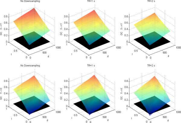
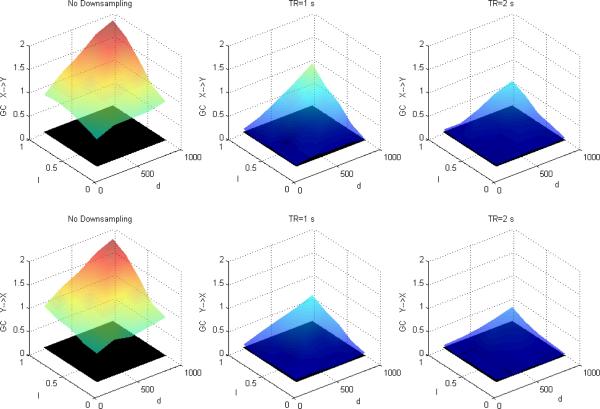
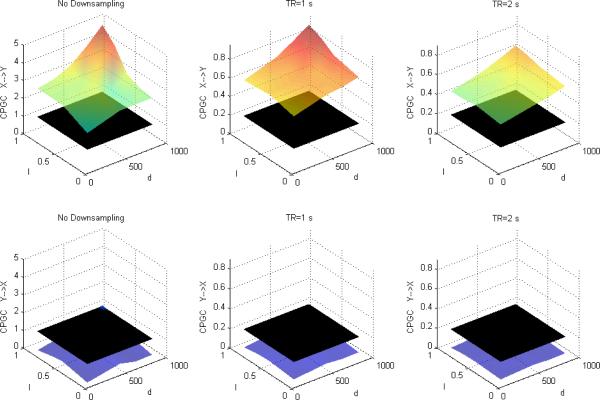
Figures 1, 2 and 3 depict DTF-based GC, Geweke's GC and CPGC values obtained from the simulated fMRI time series, respectively, with only causality (x(n)→y(n)) and no zero-lag correlation between the corresponding neuronal time series. In each of the subplots, the black surface represents the statistical threshold obtained from surrogate data [6,12,20]. GC results from Fig.1 and Fig.2 replicates the results reported in [5] where the influence from X to Y is greater than that from Y to X and the inferred causal connectivity increases as a function of I and d. However, the significant false Granger causal influence from y' (n) to x' (n) is probably due to the fact that the causal influence of x(n) on y(n) in the simulated LFP data may be inferred as being reversely causal (i.e. y' (n) to x' (n)) in the corresponding fMRI data. However, accounting for the leakage effects using CPGC eliminates the false causal influence from y' (n) to x' (n) (Fig.3) and retains the true causal influence from x' (n) to y' (n).

Figure 1.

Mean DTF-based Granger causality between simulated fMRI time series as a function of I and d without downsampling (left), with downsampling with TR=1s (middle) and TR=2s (right). The black surface represents the statistical threshold

Figure 2.

Mean Geweke's Granger causality between simulated fMRI time series as a function of I and d without downsampling (left), with downsampling with TR=1s (middle) and TR=2s (right). The black surface represents the statistical threshold

Figure 3.

Mean CPGC between simulated fMRI time series as a function of I and d without downsampling (left), with downsampling with TR=1s (middle) and TR=2s (right). The black surface represents the statistical threshold

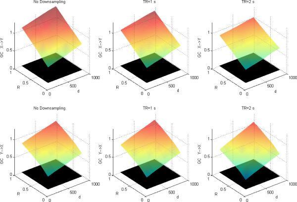
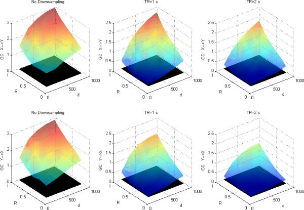
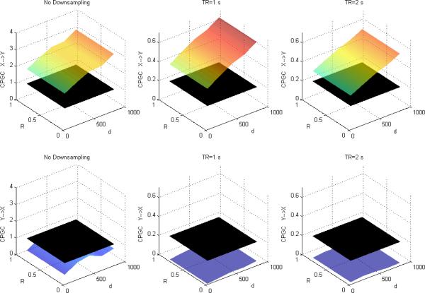
Figures 4, 5 and 6 depict DTF-based GC, Geweke's GC and CPGC values obtained from the simulated fMRI time series, respectively, with both causality (x(n)→y(n) introduced by I=0.5 and varying neuronal delay) and varying zero-lag correlation (R) between the corresponding neuronal time series. It can be observed that for both DTF-based GC and Geweke's GC, the causality was bi-directional and increased with R for a given neuronal delay. This supports our hypothesis that since IGC and GC are obtained from common parameters in Geweke's approach, the latter is influenced by the former. However, from Fig.6, CPGC remained constant with increasing instantaneous correlation but increased with neuronal delay. This demonstrates that causality derived from CPGC was not contaminated by instantaneous correlation, but accurately reflected the underlying unidirectionality and changes in the magnitude of directional influence represented by the neuronal delay.

Figure 4.

Mean DTF-based Granger causality between simulated fMRI time series as a function of R and d for fixed I=0.5 without downsampling (left), with downsampling with TR=1s (middle) and TR=2s (right). The black surface represents the statistical threshold

Figure 5.

Mean Geweke's Granger causality between simulated fMRI time series as a function of R and d for fixed I=0.5 without downsampling (left), with downsampling with TR=1s (middle) and TR=2s (right). The black surface represents the statistical threshold.

Figure 6.

Mean CPGC between simulated fMRI time series as a function of R and d for fixed I=0.5 without downsampling (left), with downsampling with TR=1s (middle) and TR=2s (right). The black surface represents the statistical threshold.

A comparison of Figures 1 and 4 (GC obtained from DTF) with Figures 2 and 5 (GC obtained from Geweke's approach) reveals that the essential information obtained from the two approaches remains the same. GC obtained from both showed that in addition to the true causal influence from X to Y, a spurious influence from Y to X was inferred. Also, longer TR and lower causal strength and neuronal delay decreased the sensitivity of GC obtained from both approaches. Therefore, even though the numerical values obtained from the two approaches were not equal, inferences obtained from them were identical, thus making the approaches equivalent.

Here we note some theoretical considerations behind the empirical evidence demonstrating the effect of zero-lag correlation on DTF-based GC, Geweke's GC and CPGC. In general, the projection of time series X on time series Y's past is supposed to capture the causal influence from Y to X. However, when X and Y are zero-lag correlated, Y's past is instantaneously related to X's past, which in turn is related to X's present due to serial correlation in X. Therefore, the relation between Y's past and X's present can be influenced by their instantaneous correlation. The fact that GC between the simulated LFP time series was insignificant even in the presence of zero-lag correlation (Table.1) suggests that due to the negative serial correlation built in the simulated system, the presence of instantaneous causality did not leak into the causal domain. However, smoothing the simulated LFP by the HRF introduces the serial correlation in the data which facilitates the leakage of zero-lag correlation into the causal domain (Table.2). Both DTF-based GC and Geweke's GC model the serial correlation, however, the way they treat instantaneous correlation is different. DTF-based GC does not model the instantaneous correlation between X and Y and hence is clearly affected by correlation leakage. Previous studies have likened instantaneous Granger causality (IGC) obtained from Geweke's framework to zero-lag correlation. However, since IGC and GC are derived from a common parameter, the variance of the VAR model error obtained from the same projection, the causality measures obtained are likely not independent of zero-lag correlation effects [3,5,21]. Geweke's GC comparatively evaluates the model errors obtained from X's projection on its own past with that obtained by X's projection on Y's past in addition to its own past. Consequently, even if Geweke's GC were to employ X's projection on Y's present, the instantaneous effect that is absorbed by the zero-lag coefficients depends on the type of projection, thus differentially altering the model errors in different projections. Therefore, the comparative evaluation of error variances ensures that Geweke's GC changes as a function of instantaneous correlation between X and Y. On the other hand, by incorporating the zero-lag terms in mVAR, the instantaneous effects are absorbed by them. However, since CPGC does not involve the comparative evaluation of model errors of two different projections as is done in Geweke's GC, the time-lagged coefficients in the mVAR do not change as a function of instantaneous correlation.

In essence, the simulations indicate that effective connectivity based on Granger causality, inferred from fMRI data, could be due to causal and/or instantaneous influences at the neuronal scale. Also, even though bidirectional interaction inferred from fMRI-based GC analysis could be due to a corresponding bidirectional neuronal interaction, a possibility always exists such that the temporal dispersion of causality caused by hemodynamic blurring makes a unidirectional neuronal causal influence appear as being bidirectional during fMRI-based GC analysis. However, it is safe to say that a causal influence inferred from fMRI-based CPGC analysis is most likely due to a corresponding neuronal causal influence. On the contrary, its absence does not rule out a neuronal causal influence because weak influences caused by small neuronal delays may not be resolvable in fMRI. Investigating the minimum resolvable neuronal latency which can be inferred from fMRI-based causality analysis is beyond the scope of this paper and will be reported elsewhere. Therefore, even though a significant CPGC path weight is a sufficient condition for inferring corresponding neuronal causality, it is not necessary.

Verbal Working Memory Networks

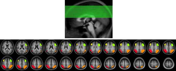
The Akaike information criterion produced an optimum order of one for the VAR model. Fig.7 shows the regions activated by the verbal working memory task and the positions of the corresponding axial slices in the brain. Fig.8 shows the thresholded networks (p<0.05) obtained from zero-lag correlation (left panel), DTF-based GC (middle panel) and CPGC (right panel). Here, we preferred to use DTF-based GC, rather than Geweke's GC, for comparison with CPGC because they are similar in methodology, i.e. both are based on the model coefficients. Paths L DLPFC ↔ L Parietal and R DLPFC ↔ L Parietal were common to both the zero-lag and GC networks with the former being retained and the latter being absent in the CPGC network. R DLPFC ↔ R Parietal and L DLPFC → R Parietal were found in both the GC and CPGC networks and L DLPFC ↔ R DLPFC is exclusive to the zero-lag network.

Figure 7.

Top panel: The positions of the slices containing the activations. Bottom panel: The regions activated by the verbal working memory task. Green: left prefrontal, Yellow: right prefrontal, Orange: left parietal, Red: right parietal

Figure 8.

Thresholded connectivity networks (p<0.05) based on zero-lag correlation (left), DTF-based Granger causality (center) and correlation-purged Granger causality (right). The p-values of the paths are indicated by the color of the arrows

The above observation demonstrates several possible scenarios. In the first scenario, a fictitious bidirectional “causal” influence between two ROIs arising in GC due to leakage of zero-lag correlation is eliminated in CPGC; this is the case for the bidirectional GC between R DLPFC and L Parietal. In the second scenario, a causal connection may be present in the absence of a significant zero-lag correlation; this may be the case for L DLPFC → R Parietal and R DLPFC ↔ R Parietal paths. In the third scenario, a relatively weaker zero-lag correlation such as that between L DLPFC and R DLPFC may not contaminate the GC results sufficiently to lead to detectable causal influences. In this case, causal influences were not detected with either GC or CPGC. In the final scenario, both zero-lag correlation and time-lagged causal influences were present and causal influences were seen in both GC and CPGC. This is illustrated by the bidirectional connection between L DLPFC and L Parietal seen in both the GC network and the CPGC network.

It is worth noting the differences between the simulations and the experimental data. First, the simulations illustrate one specific mechanism – blurring by the hemodynamic response – by which the zero-lag correlation leaks into the time-lagged domain. However, in experimental data, many such mechanisms are plausible. Specifically, our simulations assume that the effect of zero-lag correlation on time-lagged causality is linear and that the time scale of the causal influence is an order of magnitude shorter in comparison to the sampling interval of fMRI data. These assumptions may not always hold true in experimental data. However, irrespective of the mechanism of zero-lag leakage, CPGC is capable of purging the contribution of zero-lag correlation to time-lagged GC within the linear framework. Second, the instantaneous correlation in the simulated data was derived from the white innovation process while in experimental data we are most likely to encounter instantaneously mixed colored signals with non-flat spectra. Third, the simulated data used in this work were free of additive noise, which may not be the case in experimental data. It has been shown that additive noise may impact causality estimates [22] since the traditional least squares approach for obtaining the AR coefficients may be inaccurate in such circumstances [23]. Therefore, in the presence of additive noise, colored or otherwise, appropriate denoising strategies based on the Kalman filter theory and the expectation-maximization algorithm may be employed [22]. Else, an improved least squares estimation method based on combining lower order and higher order Yule-Walker equations may be used in order to accurately estimate the AR parameters in the presence of noise [23] before calculating CPGC.

Conclusions

In this study, we have assessed the effect of zero-lag correlation on time-lagged Granger causality using simulations. Furthermore, we have introduced a method, correlation-purged Granger causality, in which the zero-lag term is explicitly modeled in the VAR and subsequently omitted in calculating Granger causality. Using both simulations and fMRI data obtained during a verbal working memory task, we have demonstrated the efficacy of CPGC in compensating for zero-lag effects. Our approach allows multivariate estimation of both FC and EC in the same data set.

Bibliography

- [1].Friston KJ. Functional and effective connectivity in neuroimaging: a synthesis. Human Brain Mapping. 1995;2:56–78. [Google Scholar]
- [2].Biswal B, Yetkin FZ, Haughton VM, Hyde JS. Functional connectivity in the motor cortex of resting human brain using echo-planar MRI. Magnetic Resonance in Medicine. 1995;34(4):537–541. doi: 10.1002/mrm.1910340409. [DOI] [PubMed] [Google Scholar]
- [3].Geweke J. Measurement of Linear Dependence and Feedback Between Multiple Time Series. Journal of the American Statistical Association. 1982;77(378):304–313. [Google Scholar]
- [4].Granger CWJ. Investigating causal relations by econometric models and cross-spectral methods. Econometrica. 1969;37(3):424–438. [Google Scholar]
- [5].Roebroeck A, Formisano E, Goebel R. Mapping directed influence over the brain using Granger causality and fMRI. NeuroImage. 2005;25:230–242. doi: 10.1016/j.neuroimage.2004.11.017. [DOI] [PubMed] [Google Scholar]
- [6].Deshpande G, Hu X, Stilla R, Sathian K. Effective Connectivity during Haptic Perception: A study using Granger causality analysis of functional magnetic resonance imaging data. NeuroImage. 2008;40(4):1807–1814. doi: 10.1016/j.neuroimage.2008.01.044. [DOI] [PMC free article] [PubMed] [Google Scholar]
- [7].Stilla R, Deshpande G, Laconte S, Hu X, Sathian K. Posteromedial parietal cortical activity and inputs predict tactile spatial acuity. Journal of Neuroscience. 2007;27(41):11091–11102. doi: 10.1523/JNEUROSCI.1808-07.2007. [DOI] [PMC free article] [PubMed] [Google Scholar]
- [8].Stilla R, et al. Neural processing underlying tactile microspatial discrimination in the blind: A functional magnetic resonance imaging study. Journal of Vision. 2008;8(10):13.1–19. doi: 10.1167/8.10.13. [DOI] [PMC free article] [PubMed] [Google Scholar]
- [9].Deshpande G, LaConte S, James GA, Peltier S, Hu X. Multivariate Granger causality analysis of brain networks. Human Brain Mapping. 2009;30(4):1361–1373. doi: 10.1002/hbm.20606. [DOI] [PMC free article] [PubMed] [Google Scholar]
- [10].Deshpande G, Hu X, Lacey S, Stilla R, Sathian K. Object familiarity modulates effective connectivity during haptic shape perception. NeuroImage. 2009 doi: 10.1016/j.neuroimage.2009.08.052. in press. [DOI] [PMC free article] [PubMed] [Google Scholar]
- [11].Wang X, Chen Y, Ding M. Estimating Granger causality after stimulus onset: a cautionary note. NeuroImage. 2008;41(3):767–776. doi: 10.1016/j.neuroimage.2008.03.025. [DOI] [PMC free article] [PubMed] [Google Scholar]
- [12].Kus R, Kaminski M, Blinowska KJ. Determination of EEG activity propagation: pairwise versus multichannel estimate. IEEE Transactions on Biomedical Engineering. 2004;51(9):1501–1510. doi: 10.1109/TBME.2004.827929. [DOI] [PubMed] [Google Scholar]
- [13].Tyraskis PA, Jensen OG. Multichannel Linear Prediction and Maximum-Entropy Spectral Analysis Using Least Squares Modeling. IEEE Transactions on Geoscience and Remote Sensing. 1985;GE-23(2):101–109. [Google Scholar]
- [14].Friston KJ, Holmes AP, Ashburner J. Statistical Parametric Mapping (SPM) 1999 [Online]. http://www.fil.ion.ucl.ac.uk/spm/
- [15].Logothetis NK, Pauls J, Augath M, Trinath T, Oeltermann A. Neurophysiological investigation of the basis of the fMRI signal. Nature. 2001;412:150–157. doi: 10.1038/35084005. [DOI] [PubMed] [Google Scholar]
- [16].Kaminski M, Ding M, Truccolo W, Bressler S. Evaluating causal relations in neural systems: Granger causality, directed transfer function and statistical assessment of significance. Biological Cybernetics. 2001;85:145–157. doi: 10.1007/s004220000235. [DOI] [PubMed] [Google Scholar]
- [17].Granger CWJ, Hatanaka M. Spectral Analysis of Economic Time Serie. Princeton University Press; New Jersey: 1964. [Google Scholar]
- [18].Friston KJ, Jezzard P, Turner R. Analysis of functional MRI time series. Human Brain Mapping. 1994;2:69–78. [Google Scholar]
- [19].Talairach J, Tournoux P. Co-Planar Stereotaxic Atlas of the Human Brain. Thieme Medical Publishers; New York: 1988. [Google Scholar]
- [20].Theiler J, Eubank S, Longtin A, Galdrikian B, Farmer D. Testing for nonlinearity in time series: The method of surrogate data. Physica D. 1992;58:77–94. [Google Scholar]
- [21].Rajagovindan R, Ding M. Decomposing Neural Synchrony: Toward an Explanation for Near-Zero Phase-Lag in Cortical Oscillatory Networks. PLoS ONE. 2008;3(11):e3649. doi: 10.1371/journal.pone.0003649. [DOI] [PMC free article] [PubMed] [Google Scholar]
- [22].Nalatore H, Ding M, Rangarajan G. Mitigating the effects of measurement noise on Granger causality. Physical Review E. 2007;75:031123–1. 031123–10. doi: 10.1103/PhysRevE.75.031123. [DOI] [PubMed] [Google Scholar]
- [23].Mahmoudi A, Karimi M. Parameter estimation of autoregressive signals from observations corrupted with colored noise. Signal Processing. 2010;90:157–164. [Google Scholar]