Spatial and temporal separation fails to counteract the effects of low prevalence in visual search

Abstract

Recent research has shown that, in visual search, participants can miss 30–40% of targets when they only appear rarely (i.e. on 1–2% of trials). Low target prevalence alters the behavior of the searcher. It can lead participants to quit their search prematurely (Wolfe et al., 2005), to shift their decision criteria (Wolfe et al., 2007) and/or to make motor or response errors (Fleck & Mitroff, 2007). In this paper we examine whether the LP Effect can be ameliorated if we split the search set in two, spreading the task out over space and/or time. Observers searched for the letter “T” among “L”s. In Experiment 1, the left or right half of the display was presented to the participants before the second half. In Experiment 2, items were spatially intermixed but half of the items were presented first, followed by the second half. Experiment 3 followed the methods of Experiment 2 but allowed observers to correct perceived errors. All three experiments produced robust low prevalence (LP) effects with higher errors at 2% prevalence than at 50% prevalence. Dividing up the display had no beneficial effect on errors. The opportunity to correct errors reduced but did not eliminate the LP effect. Low prevalence continues to elevate errors even when observers are forced to slow down and permitted to correct errors.

Introduction

Humans perform visual search tasks regularly. Examples of these tasks range from searching for a particular brand of food at a supermarket or for a friend in a busy street. Selective attentional mechanisms can be used to parse out irrelevant information to help us find what we are looking for. In general, we perform these tasks quite well. However, our ability to find a target can depend on how frequently it appears. Recent research (e.g. Wolfe et al., 2005) has shown that participants miss targets that appear rarely (“low prevalence targets”) more than targets that appear more frequently (“high prevalence targets”). Many socially important search tasks are low prevalence searches; including medical screening tests for breast and cervical cancer (e.g., Fenton et al., 2007) and baggage screening for threats at an airport. Thus, a tendency to miss infrequent targets could have serious effects.

In their first studies of low prevalence search, Wolfe, Horowitz and Kenner (2005) used visually complex search displays, intended to mimic x-rayed baggage. In their original displays, participants were searching for a tool among other categories of objects. In a Low Prevalence condition, with targets that appeared on only 1% of trials, the proportion of miss errors was 0.30 compared to just 0.07 at high (50%) prevalence. This ‘Low Prevalence’ (LP) Effect (i.e. the elevation of miss errors when the target is rare compared to when it is common) has been replicated on several occasions with both complex and simple stimuli (e.g. Fleck & Mitroff, 2007; Rich, Kunar, Van Wert, Hidalgo-Sotelo, Horowitz, & Wolfe, 2008; Wolfe et al., 2007 and Van Wert et al, 2009).

Initially, it seemed as though the LP Effect could be explained as a speed-accuracy trade-off. Target-absent RTs are dramatically shorter under LP conditions and the rise in miss errors might be a simple consequence of too rapid a termination of search. Supporting this account of the LP Effect, Fleck and Mitroff (2007) found that their participants actually recognized when they had responded “absent” too quickly and missed a target item. When given the chance to change their responses, they could abolish the LP Effect. The picture becomes more complex if a more difficult search task is used. A simple speed-accuracy trade-off would result in a loss of sensitivity (using the term in its signal detection sense to refer to a decrease in d’ and/or the area under an ROC curve). However, Wolfe et al. (2007), using a baggage search task, found that false alarm error rates decreased as miss error rates increased at LP. Sensitivity changed very little. In fact, if d’ is used as the measure, sensitivity increased at LP. The trading of false alarm for miss errors is consistent with a criterion shift that causes participants to respond “absent” more readily at LP. Indeed in non-search tasks, prevalence is known to alter decision criterion, rather than sensitivity (Healy & Kubory, 1981; Maddox, 2002; Treisman, 1984). The pattern of effects of prevalence in visual search becomes clearer when very high prevalence conditions are included. Wolfe and Van Wert (2009) include prevalence rates as high as 98%. At 98% prevalence, miss error rates are very low and false alarm error rates are markedly elevated. Given that target-absent RTs are very fast at low prevalence, one might expect target-present RTs to become very fast at very high prevalence, but that is not what happens. Target-present RTs change very little as a function of prevalence. Instead, the target-absent RTs become dramatically slower at very high prevalence.

Wolfe and Van Wert (2009) presented a two-threshold account of these data cartooned for the case of a search for a “T” among “L”s – the task that is used in this paper (see Figure 1). In this account, prevalence changes a decision criterion and a search termination threshold. The decision threshold is used to determine whether an item is categorized as a target or not (here, a T or an L). If it is determined to be a target, the search ends with a “target-present” response. If an item is not categorized as a target, search continues. The two-threshold model proposes that a separate signal accumulates toward a search termination threshold. When that threshold is exceeded search is ended with a target-absent response. If that threshold is not exceeded, search continues with a new selection. Under LP conditions, the decision criterion moves to the right, making it less likely that an item will be labelled as a target and the quitting threshold drops, making absent RTs faster.

Figure 1.

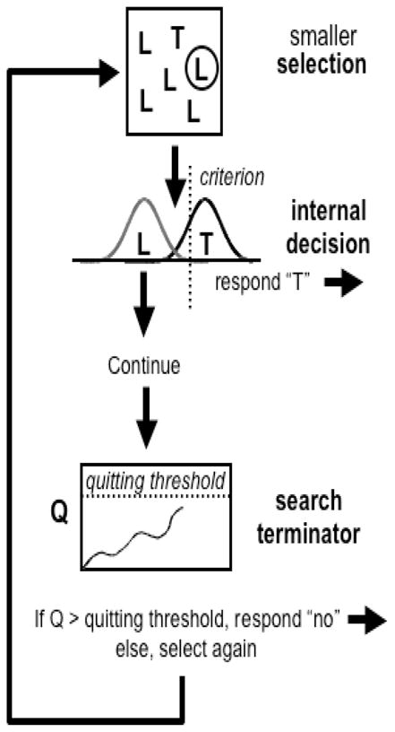
Schematic representation of the observed criterion shift in LP trials. With an increase in target absent trials participants are less likely to declare that a target is present, leading the decision criterion to become more conservative. With a more conservative criterion there will be fewer false alarms but also fewer hits (i.e. more miss errors). Note that there is little effect of sensitivity (as measured by d’) with a reduction in target prevalence.

In this paper, we ask whether we can improve performance by separating the visual display over two dimensions: space and time. In particular, we ask if it is possible to reduce the miss errors that characterize the LP Effect. It is well known that participants can use both spatial and temporal cues to aid visual search. Participants can allocate their visual attention to specific spatial areas, which leads to better detection of the target (e.g. Posner et al., 1980). Furthermore, participants can use temporal cues to sub-divide the display into groups, allowing attention to be applied to one temporal group over the other (e.g. Jiang, Chun & Marks, 2002). The present experiments investigate whether participants can make use of these visual cues to eliminate the Low Prevalence Effect. If part of the LP Effect occurs because the quitting threshold drops, causing participants respond too soon, then perhaps splitting the display across space and time (and providing segmenting visual cues) will encourage participants to more fully search each part of the display, improving target detection. In Experiment 1, we presented half the items on one side of the display first, followed by the other half, so that the two parts of the display were spatially, as well as temporally separate. In Experiment 2, the display was randomly presented across the whole computer display in two asynchronous groups, so that the display could be segregated into two temporal presentations. The former is analogous to a baggage-screener seeing half the bag at a time as it moves through the scanner. Finally, in Experiment 3, participants were given the option to correct perceived response errors. To preview the results, the data suggest that neither spatial nor temporal segmentation of the display eliminates the LP Effect.

Experiment 1: Splitting the display across space and time

Method

Participants

Twelve naive observers took part in Experiment 1. All participants met our general age range criterion of being between 18 and 55 years old (Mean age = 28.3, SD = 7.6), had normal or corrected to normal vision and were paid for their time. Informed consent was obtained from all observers.

Stimuli and Procedure

Experiment 1 was conducted on a Macintosh computer using Matlab Software with the PsychToolbox (Brainard, 1997; Pelli, 1997). All stimuli subtended 1.2° × 1.2° at a viewing distance of 57 cm and were presented on a uniform dark grey background. The distractor items were white L shapes and the target item (if present) was a white T shape. All stimuli were presented randomly in one of four orientations (0, 90, 180 or 270 degrees) with equal probability. Each L contained a small offset (approximately 0.1 degree) at the line junction to make search more difficult (see Figure 2). The overall size of the display was 20 deg × 20 deg. It was divided into an invisible 6 × 6 matrix for purposes of stimulus placement.

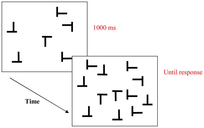
Figure 2.

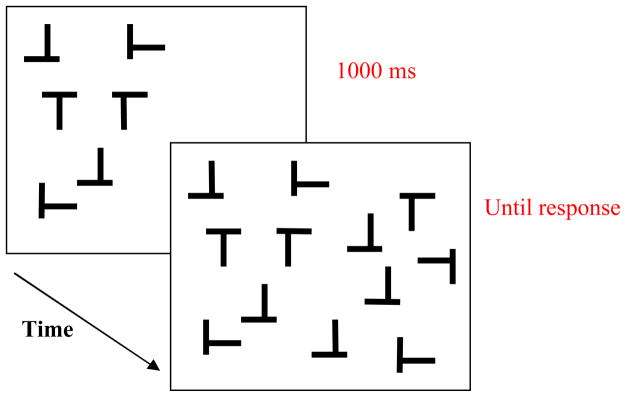
Example displays of the Half condition for Experiment 1 in which one side of the display appeared initially, followed by the other side of the display after 1000 msec. Participants were instructed to search for the target letter T.

There were two conditions – a Half condition and a Whole condition. In the ‘Half’ condition, half of the stimuli appeared for 1000 msec (‘the first set’) followed by the other half of the stimuli (‘the second set’). Six letters appeared initially followed by six more letters to produce a total set size of 12. Within this 1000 msec time frame participants should have ample time to search through the first set of items before the second set was added. Once the second set was presented, both sets remained on the screen until response. The target could appear in either the first or the second set and thus the first or second part of the display. The first set was presented on one side of the screen followed by the second set, presented on the other side of the screen, so that the presentations of stimuli were spatially separate (see Figure 2). For half the participants the first set appeared on the left hand side of the screen followed by the second set on the right hand side of the screen; for the other half of participants it was vice versa. Participants could only respond after the second part of the display appeared and all stimuli remained visible until response. Participants were instructed to press one key if the target was present and another key if the target was absent, and to respond as quickly but as accurately as possible. A white fixation dot was presented for 500 msec prior to each search display.

The Whole conditions were similar to the Half conditions but here all the stimuli appeared at the same time. There were two whole conditions: one condition where 6 items appeared anywhere on the screen (‘Whole - SS 6’) and one condition where 12 items appeared anywhere on the screen (‘Whole – SS 12’). These conditions were used to control for the difference in set size across the presentations in the Half condition.

Each condition was run in blocks of high and low prevalence. Each participant completed all four of the trial blocks: Half–HP, Half-LP, Whole-HP and Whole-LP The experiment took approximately 4 hours to complete spread over 2 or more days. The presentation of the Half and Whole conditions were scheduled so that half of the participants completed the Half conditions before the Whole conditions. The presentation order was reversed for the other half of the participants. Within each session the order of the HP and LP trials was also counterbalanced across participants. At High Prevalence (HP) the target appeared 50% of the time; at Low Prevalence (LP) the target only appeared 2% of the time. Each Half HP condition contained 80 trials (20 trials where the target was present in the first set, 20 trials where the target was present in the second set and 40 target absent). For the Half LP conditions there were 2000 trials (20 trials where the target was present in the first set, 20 trials where the target was present in the second set and 1960 target absent). Each Whole HP condition contained 160 trials (40 target present and 40 target absent per set size). The Whole LP conditions contained 2000 trials (20 target present and 980 target absent per set size). Feedback about accuracy was given to the observer on every trial. Breaks were enforced every 200 trials so that HP sessions were similar in duration to the longest sustained part of an LP session. Thus, differences between HP and LP were not due to observer fatigue – at least, not fatigue due to lack of a break. Trials automatically timed out after 10 seconds if participants did not respond.

Results and Discussion

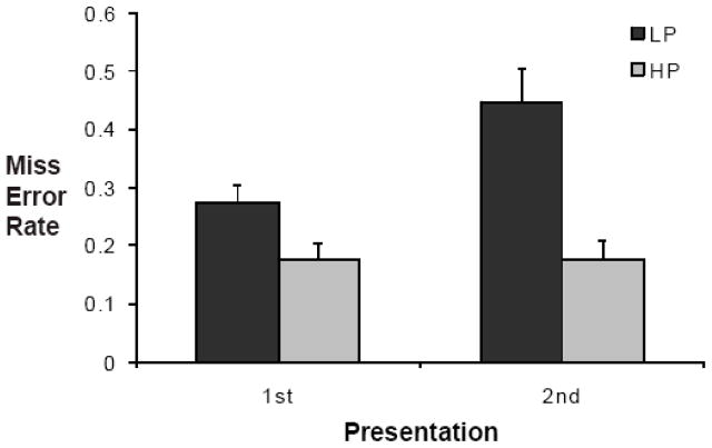
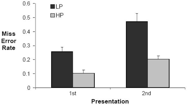
The critical result is shown in Figure 4. Splitting the display into two halves did not eliminate the prevalence effect.

Figure 4.

Miss error rates for the Half conditions for Experiment 1. In this experiment there was no option to correct the response. Error bars represent the standard error.

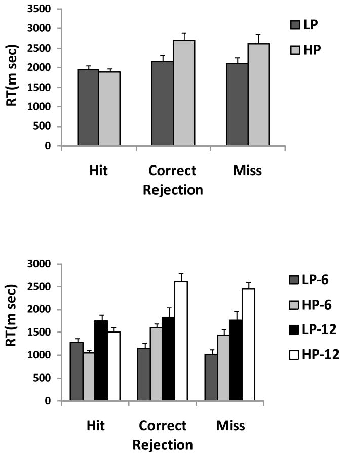
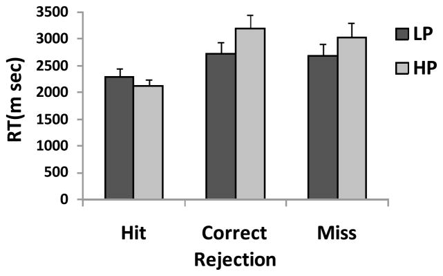
Trials with RTs less than 200 msec or greater than 5000 msec were removed as outliers (1.3% of the data, 0.02% of these trials were less than 200 msec). RTs are plotted in Figure 3. LP trials have faster RTs than HP trials, F(1,11) = 5.1, p < 0.05 and the target-present trials have faster RTs than target-absent trials, F(1,11) = 23.8, p < 0.01. The Prevalence × Target Presence interaction was also significant, F(1,11) = 51.1, p < 0.01. Most notably, RTs on correct target absent trials under LP conditions were faster than under HP conditions, t(11) = 4.0, p < 0.01, following the same pattern seen in previous prevalence studies. Unsurprisingly as participants had more time to prepare a response, RTs were faster when the target appeared in the first presentation than when it appeared in the second presentation (for HP: 1497 vs 2290 msec; for LP: 1560 vs 2397 msec, both ts > 10, ps < 0.01). We will return to the RTs in the General Discussion.

Figure 3.

(a) Overall RT in milliseconds for hit, correct rejection and miss responses for the Half condition of Experiment 1 and (b) RT in milliseconds for hit, correct rejection and miss responses for the Whole conditions of Experiment 1. Error bars represent the standard error.

Our primary interest is why people miss a greater proportion of targets in low prevalence search. Thus, we will focus on the observed miss error rates. With this task, false alarm errors were minimal (less than 2% in all conditions) and as such were not analysed further. In all experiments, miss errors were arcsine transformed before analysis to compensate for unequal variances present in binomial data (Hogg & Craig, 1995). The means shown in Figure 4 are back-transformed data. An ANOVA of the Half condition with factors of Prevalence (LP vs HP) and Presentation (target in the first half vs second half of the display) show that there was a main effect of Prevalence: participants missed a greater proportion of the targets in the LP condition than in the HP condition, F(1, 11) = 37.8, p < 0.01., but not of Presentation F(1, 11) = 3.2, p = 0.1. The Prevalence × Presentation interaction, however, was significant, F(1,11) = 8.8, p < 0.05: participants missed more targets in the second part of the display than the first at LP, t(11) = 2.4, p < 0.05, but not at HP, t(11) = 0.0, p = n.s..

Was the difference in LP error rates across presentation due to a simple speed-accuracy trade-off? For the “speed” aspect of this equation, we find the difference between LP and HP RTs for correct target absent trials. A larger difference indicates that an observer speeded up more dramatically at low prevalence. Does that difference correlate with the miss error rate? When the target appears in the first half, the answer is no (r-sq = 0.04, t(10) = 0.6, p = 0.53). However, when the target is in the second half, the correlation almost rises to statistical significance (r-sq = 0.31, t(10) = 2.1, p = 0.06).

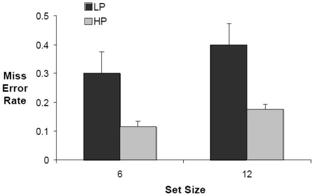
Our main goal was to determine if presenting twelve items in two successive appearances of six items is better than presenting twelve items all at once. Figure 5 shows the results for the standard presentation of 6 and 12 items (in the whole conditions). It is clear that the general pattern of results and the overall rates of errors are comparable in the 6 and 12 conditions and the first half /second half conditions of Figure 4. In an ANOVA on the 6 and 12 conditions, there were main effects of Prevalence: more miss errors at low prevalence than high prevalence, F(1,11) = 12.9, p < 0.01, and of Set Size: more miss errors at the larger set size than smaller set size, F(1, 11) = 14.9, p < 0.01.

Figure 5.

Miss error rates for the Whole conditions of Experiment 1. Here all the stimuli were presented at once. There were two set sizes (set size 6 and 12). Error bars represent the standard error.

To test for a benefit of splitting the display across space and time, we compared LP error rates between the split and equivalent single set size version of the task in order to determine if there was any improvement in the detection of LP targets when the display was separated. A paired t-test between the Whole set size 12 and the separated display showed no difference in miss errors between these conditions, t(11) = 1.1, p = 0.3. Splitting the display up across space and time did little to benefit LP search.

Experiment 2: Splitting the display across time

In Experiment 1, the displays are separated across space and time. Experiment 2 investigates if the same results are found when the separation occurs only in time.

Participants

Twelve naïve observers took part in Experiment 2. All participants were aged between 18 and 55. The average age for eleven of the participants is 32.8 years (SD 9.1 years). We are missing the age of one observer. All had normal or corrected to normal vision and were paid for their time. Informed consent was obtained from all observers.

Stimuli and Procedure

The stimuli and procedure for the Half conditions in Experiment 2 were similar to that of Experiment 1 except that the items in the first set could appear anywhere within the display area (i.e. they were not limited by side) and these were followed by the second set that could also appear anywhere on the screen (with the caveat that they could not occlude the first set, see Figure 6). There were no Whole conditions. The experiment took approximately 2 hours to complete and the order of HP and LP blocks was counterbalanced across participants.

Figure 6.

Example displays of the Half condition for Experiments 2 and 3, in which half the stimuli appeared initially. The stimuli could appear anywhere in the display and were not restricted to a side. After 1000 msec the other half of the stimuli were added.

Results and Discussion

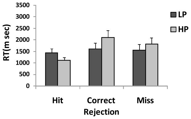
Data from Experiment 2 showed a similar pattern to that of Experiment 1. RTs below 200 msec and above 5000 msec were removed as outliers. This led to the removal of 5.1% of the data (0.02% of trials were less than 200 msec). RTs are plotted in Figure 7 and were faster when the target was present, F(1,11) = 40.9, p < 0.01. There was no main effect of prevalence on RTs, F(1,11) = 1.2, p = n.s., however, the Prevalence × Target Presence interaction was significant, F(1,11) = 25.9, p < 0.01. Again, RTs on correct target absent trials under LP conditions were faster than under HP conditions, t(11) = 3.4, p < 0.01, following the same pattern seen in previous prevalence studies. As in Experiment 1, RTs were faster, when the target appeared in the first presentation than when it appeared in the second presentation (for HP: 1690 vs 2605 msec; for LP 2049 vs 2681 msec, both ts > 5, ps < 0.01).

Figure 7.

Overall RT in milliseconds for hit, correct rejection and miss responses for the Experiment 2. Error bars represent the standard error.

Figure 8 shows the miss error data from Experiment 2. An ANOVA showed that, like Experiment 1, there was a main effect of Prevalence, F(1, 11) = 33.8, p < 0.01. Participants made more errors at LP than at HP. Participants also missed the target more if it appeared in the second part of the display compared to the first, F(1, 11) =25.8, p < 0.01. The Prevalence × Presentation interaction was not significant, F(1,11) = 0.4, p = n.s.. Planned comparisons showed that in both the LP and HP conditions participants made more errors when the target appeared in the second part of the display compared to the first (LP: t(11) = 4.4, p < 0.01 and HP: t(11) = 2.7, p < 0.05). As in Experiment 1, we subtracted mean LP RTs for correct target absent trials from HP as a measure of the change in quitting threshold between HP and LP. In Experiment 2, there were significant correlations between the miss errors and this measure for targets appearing in the first presentation (r-sq = 0.35, t(10) = 2.3, p < 0.05) and the second presentation (r-sq = 0.57, t(10) = 3.6, p < 0.01).

Figure 8.

Miss error rates for the Half conditions for Experiment 2. In this experiment there was no option to correct the response. Error bars represent the standard error.

A direct comparison of Experiments 1 and 2 shows there was no effect of presenting the stimuli spatially separated versus distributed across the whole screen – especially at Low Prevalence. Again, there was an overall effect of Prevalence, F(1,22) = 69.9, p < 0.01, an effect of Presentation, F(1, 22) = 20.1, p < 0.01, and a significant Prevalence × Presentation interaction, F(1, 22) = 5.3, p < 0.05. However, critically for this analysis, there was no overall main effect of Experiment, F(1, 22) = 0.4, p = n.s.. Nor were any of the interactions with the Experiment factor significant (e.g. spatially separate vs. distributed, all Fs < 2.6). The additional visual cue of spatial separation did little to improve target detection.

Clearly, splitting the display in half and displaying those halves sequentially does not reduce the LP Effect. It may, however, produce some insight into the effect of low prevalence. The miss errors are more likely to occur when the target is in the second half of the display than in the first. This could indicate a rising pressure to quit as the trial progresses. In the final experiment, we test whether these elevated second half errors are correctable motor / response errors of the sort reported by Fleck and Mitroff (2007).

Experiment 3: Self-correction response

In Experiment 3, participants were given the option to self-correct their mistakes by pressing the ‘escape’ key (akin to the methodology of Fleck & Mitroff, 2007).

Participants

Ten naive observers took part in Experiment 2. All participants were aged between 18 and 55 (Mean age = 21.0, SD = 1.4), had normal or corrected to normal vision and were paid for their time. Informed consent was obtained from all observers.

Stimuli and Procedure

The stimuli and procedure were similar to that of Experiment 2 except that in Experiment 3 there was no feedback and participants were given the option to change their response if they wished by pressing the ‘escape’ key. This had the consequence of reversing the response of the previous trial following the methodology of Fleck & Mitroff (2007). Both the Initial Errors and the Corrected Errors were recorded. Experiment 3 was conducted on a PC using Blitz Basic. All stimuli subtended 1.6° × 1.6° at a viewing distance of 57 cm and were presented on a uniform black background. Like Experiment 2, there were no Whole conditions. The experiment took approximately 2 hours to complete and the order of the HP and LP blocks were counterbalanced across participants.

Results and Discussion

RTs below 200 msec and above 5000 msec were removed as outliers. This led to the removal of 3.5% of the data (1.1% of the trials were less than 200 msec). RTs are plotted in Figure 9 and were faster when the target was present, F(1,9) = 20.6, p < 0.01. There was no main effect of prevalence on RTs, F(1,9) = 0.4, p = n.s., however, the Prevalence × Target Presence interaction was significant, F(1,9) = 20.4, p < 0.01. Again, RTs on correct target absent trials under LP conditions were faster than under HP conditions, t(9) = 2.5, p < 0.05, following the same pattern seen in previous prevalence studies. RTs were faster, when the target appeared in the first presentation than when it appeared in the second presentation (for HP: 689 vs 1381 msec; for LP 1009 vs 1688 msec, both ts > 11, ps < 0.01).

Figure 9.

Overall RT in milliseconds for hit, correct rejection and miss responses for the Experiment 3. Error bars represent the standard error.

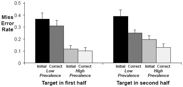
Figure 10 shows the miss error data from Experiment 3. Similar to Fleck and Mitroff’s (2007) findings, miss errors were significantly reduced after correction compared to initial errors, F(1, 9) = 29.4, p < 0.01, suggesting that at least some of these errors should be classified as motor / response errors. Correction resulted in reduced error rates in both the first and second presentations at LP and also in the 2^nd presentation at HP (all t(9) = > 3.3, p < 0.01). However, consistent with VanWert et al. (2009), the LP Effect was not eliminated by offering the self-correction option. Even after correction, LP error rates were significantly higher than HP error rates when the target appeared in either the first display, t(9) = 3.0, p < 0.02, or in the second display, t(9) = 3.2, p < 0.02. Thus, correctable motor errors did not account for the entire observed LP Effect in this experiment.

Figure 10.

Miss error rates for Experiment 3 showing both the Initial error rates and the Corrected (‘Correct’) error rates. Error bars represent the standard error.

In Experiment 3, the overall pattern of errors changed somewhat from Experiment 2. In Experiment 2, there were many more errors when the target appeared in the second half of the display. This was not true in Experiment 3 where there was no effect of Presentation on errors (1^st half vs 2^nd half, F(1, 9) = 1.2, p = n.s.). Nor was there a Prevalence × Presentation interaction, F(1, 9) = 1.9, p = n.s.. The effect of correction was greater in the second half than in the first, suggesting that the elevated errors in the second halves of Experiments 1 and 2 might have been due, at least in part, to motor / response mistakes.

As before, we subtract LP correct target absent RTs from HP correct target absent RTs as a measure of LP speeding. When we correlate this measure with miss error rates in Experiment 3, we find no significant relationship for the first or second presentation (1^st: r-sq = 0.06 and 2^nd: r-sq = 0.0, both ts < 1). Thus, with the ability to correct, there is no elevation of errors in the second half of the presentation and no evidence for a relationship between speeding of response and 2^nd half errors.

Interestingly, indications of a speed-accuracy trade-off can be found elsewhere in Experiment 3. When examining the correlations for the LP RTs to find the targets with their respective miss errors, although the correlation for the second presentation was not significant (r-sq = 0.3, t(8) = 1.7, p = 0.1), there was a significant correlation for the first presentation (r-sq = 0.6, t(8) = 3.2, p = 0.01). Miss errors were increased at shorter RTs when the target appeared in the first display. This may explain why miss errors were equated for the first and second presentations in Experiment 3 but not in Experiment 1 and 2 (where these correlations were not significant). A speed-accuracy trade-off in the first presentation may have raised the miss errors observed so that they were similar to those in the second presentation. We address this further in the General Discussion.

General Discussion

These three experiments support several conclusions. First and most practically, we failed to eliminate the LP effect by spatially and/or temporally dividing the display. A robust LP Effect was found in both display presentations. Thus, a strategy of forcing observers to look at one half of a stimulus (e.g. a bag in airport screening) before the other is unlikely to produce a benefit. It has been proposed that LP conditions make observers less likely to classify a target as a target, reducing the hit rate (Wolfe et al., 2007). In other tasks, this is accompanied by a decrease in the chance of classifying a distractor as a target, so the false alarm rate drops. However, this task produces very few false alarms so that effect is not seen here.

LP conditions also induce observers to quit search more quickly. In Experiments 1 and 2, this seems to produce especially elevated miss errors when the target is in the second set of items. This miss rate is significantly correlated with the amount of speeding in Experiment 2 and there is a similar trend in Experiment 1. In Experiment 3, when observers can correct their errors, the pattern of errors changed. The second half errors were no longer elevated relative to the first half and no longer correlated with the speeding of response. Nevertheless, regrettably, even in Experiment 3, splitting the display did not eliminate the LP effect. Before completely abandoning this approach, it is worth noting that this experiment used simple stimuli with small set sizes. It is possible that a benefit might be visible with a more difficult task (see Forlines & Balakrishnan, 2009).

One might think that, at the very least, performance on the first half of the displays should have been improved. After all, observers were being forced to spend a full second on the first half before the second half appeared. Yet an LP Effect still occurred. Previous work has reported a similar failure to cure any such trade-off by slowing the task. Wolfe et al. (2007) enforced “speed limits”, slowing observers in the LP condition to roughly the same RT as in HP conditions. This did not significantly reduce the LP Effect (see also Rich et al., 2008, who had participants wait 2 seconds after the onset of the display before they could make a response). In the present experiments, observers could not make a response during the full second that the first half of the display was present. Apparently, they did not use that extra time in profitable search. You can bring the eyes to the stimulus, but you can’t make them search.

It is also worth noting that, in the present experiments, large LP Effects occurred with a simple search for a T among Ls. This points to the robustness of the LP Effects. Moreover, the failure of the opportunity for correction to eliminate the LP effect in Experiment 3 adds another level of complexity. Recall that Fleck and Mitroff (2007) found that allowing correction eliminated the LP effect. Van Wert et al. (2009) in contrast, reported that correction did not eliminate the LP effect when they used a harder task that produced false alarms. They argued that simple tasks might produce motor/response errors but that the LP effect in more difficult tasks represented a different response to the pressure of low prevalence. In the present experiment, observers produced very few false alarms at HP (< 2% in each experiment) or LP (<1% in each experiment). Even in this simple task, correction did not eliminate the prevalence effect though it did significantly reduce it. It seems that the pressure of the LP condition produced some response errors that could be pulled back if observers were given the chance (suggesting at least a contribution of motor response errors to the LP Effect), but other LP miss errors represent other types of search failure. LP conditions can make observers quit too soon (Wolfe et al., 2005), shift their criterion (Wolfe et al, 2007), or push the wrong key (Fleck and Mitroff, 2007). Breaking up the task into two halves certainly slows the search. However, it fails to alleviate the pressure of searching for something very rare.

References

- Brainard DH. The Psychophysics Toolbox. Spatial Vision. 1997;10:443–446. [PubMed] [Google Scholar]
- Fenton JJ, Taplin SH, Carney PA, Abraham L, Sickles EA, D’Orsi C, et al. Influence of computer-aided detection on performance of screening mammography. New England Journal of Medicine. 2007;356(14):1399–1409. doi: 10.1056/NEJMoa066099. [DOI] [PMC free article] [PubMed] [Google Scholar]
- Fleck MS, Mitroff SR. Rare targets are rarely missed in correctable search. Psychological Science. 2007;18:943–947. doi: 10.1111/j.1467-9280.2007.02006.x. [DOI] [PubMed] [Google Scholar]
- Forlines C, Balakrishnan R. Improving visual search with image segmentation. Chi2009: Proceedings of the 27th annual Chi conference on human factors in computing systems; 2009. pp. 1093–1102. [Google Scholar]
- Jiang Y, Chun MM, Marks LE. Visual marking: Selective attention to asynchronous temporal groups. Journal of Experimental Psychology: Human Perception and Performance. 2002;28:717–750. [PubMed] [Google Scholar]
- Healy AF, Kubory M. Probability matching and the formation of conservative decision rules in a numerical analog of signal detection. Journal of Experimental Psychology: Human Learning and Memory. 1981;7:344–354. [Google Scholar]
- Hogg RV, Craig AT. Introduction to mathematical statistics. 5. Upper Saddle River, NJ: Prentice-Hall; 1995. [Google Scholar]
- Maddox WT. Toward a unified theory of decision criterion learning in perceptual categorization. Journal of Experimental Analysis of Behavior. 2002;78:567–595. doi: 10.1901/jeab.2002.78-567. [DOI] [PMC free article] [PubMed] [Google Scholar]
- Pelli DG. The VideoToolbox software for visual psychophysics: Transforming numbers into movies. Spatial Vision. 1997;10:437–442. [PubMed] [Google Scholar]
- Posner M, Snyder C, Davidson B. Attention and the detection of signals. Journal of Experimental Psychology: General. 1980;109:160–174. [PubMed] [Google Scholar]
- Rich AN, Kunar MA, Van Wert M, Hidalgo-Sotelo B, Horowitz T, Wolfe JM. Why do we miss rare targets? Exploring the boundaries of the low prevalence effect. Journal of Vision. 2008;8(15):1–17. doi: 10.1167/8.15.15. [DOI] [PMC free article] [PubMed] [Google Scholar]
- Treisman M. A theory of criterion setting: An alternative to the attention band and response ratio hypotheses in magnitude estimation and cross-modality matching. Journal of Experimental Psychology: General. 1984;113:443–463. doi: 10.1037//0096-3445.113.3.443. [DOI] [PubMed] [Google Scholar]
- Treisman A, Gelade G. A feature-integration theory of attention. Cognitive Psychology. 1980;12:97–136. doi: 10.1016/0010-0285(80)90005-5. [DOI] [PubMed] [Google Scholar]
- VanWert MJ, Wolfe JM, Horowitz TS. Even in correctable search, some types of rare targets are frequently missed. Attention, Perception & Psychophysics. 2009;71(3):541–553. doi: 10.3758/APP.71.3.541. [DOI] [PMC free article] [PubMed] [Google Scholar]
- Wolfe JM, Horowitz TS, Kenner NM. Rare items often missed in visual searches. Nature. 2005;435(7041):439–440. doi: 10.1038/435439a. [DOI] [PMC free article] [PubMed] [Google Scholar]
- Wolfe JM, Horowitz TS, Van Wert MJ, Kenner NM, Place SS, Kibbi N. Low target prevalence is a stubborn source of errors in visual search tasks. Journal of Experimental Psychology: General. 2007;136(4):623–638. doi: 10.1037/0096-3445.136.4.623. [DOI] [PMC free article] [PubMed] [Google Scholar]
- Wolfe JM, VanWert MJ. Varying target prevalence reveals two, dissociable decision criteria in visual search. Current Biology. 2009 doi: 10.1016/j.cub.2009.11.066. Resubmitted August 2009. [DOI] [PMC free article] [PubMed] [Google Scholar]