

Abstract
An approach for efficient and accurate finite element analysis of harmonically excited soft solids using high-order spectral finite elements is presented and evaluated. The Helmholtz-type equations used to model such systems suffer from additional numerical error known as pollution when excitation frequency becomes high relative to stiffness (i.e. high wave number), which is the case, for example, for soft tissues subject to ultrasound excitations. The use of high-order polynomial elements allows for a reduction in this pollution error, but requires additional consideration to counteract Runge's phenomenon and/or poor linear system conditioning, which has led to the use of spectral element approaches. This work examines in detail the computational benefits and practical applicability of high-order spectral elements for such problems. The spectral elements examined are tensor product elements (i.e. quad or brick elements) of high-order Lagrangian polynomials with non-uniformly distributed Gauss-Lobatto-Legendre nodal points. A shear plane wave example is presented to show the dependence of the accuracy and computational expense of high-order elements on wave number. Then, a convergence study for a viscoelastic acoustic-structure interaction finite element model of an actual ultrasound driven vibroacoustic experiment is shown. The number of degrees of freedom required for a given accuracy level was found to consistently decrease with increasing element order. However, the computationally optimal element order was found to strongly depend on the wave number.
Keywords: spectral elements, high-order, finite element method, Helmholtz, high wave number, soft tissue
1. Introduction
Understanding the response of soft solids under high frequency harmonic excitation has become of particular importance to medical science due to the advent and expanded uses of diagnostic techniques that rely on wave propagation phenomena to elucidate information about tissue properties. For example, two promising developing technologies for imaging and characterization of the mechanical properties of soft biological tissue are Magnetic Resonance Elastography (MRE) [1, 2] and Vibroacoustography (VA) [3]. In MRE, low frequency (tens to hundreds of Hz) monochromatic waves are induced in the tissue through direct mechanical coupling. The ensuing response is measured spatially using MR. Sinkus and coworkers [1, 2] have used this technique for estimating viscoelastic and elastic properties in breast tissue with the goal of differentiating benign and malignant tumors. In VA, high frequency (kHz range) harmonic radiation force is generated through two intersecting ultrasound beams, and the resulting acoustic emissions of the vibrated tissue are monitored. For imaging purposes, the ultrasound force is focused at various points throughout the tissue and the variation in acoustic emissions is plotted. Stimulation of tissue using the radiation force of ultrasound has gained wide attention for different applications due to its noninvasive character and controllable and broad range of excitation frequencies [4, 5, 6, 7, 8].
The finite element method (FEM) is the natural choice to model the propagation of waves in complex structures such as biological tissue because of the capabilities to simply account for complex geometries, material heterogeneity, and anisotropy, among other benefits. Furthermore, performing simulations in the frequency domain is typically preferable when a steady-state behavior is expected to avoid unnecessary and costly time integration. However, FEM has been found to have computational difficulties when dealing with the steady-state dynamic analysis of soft materials excited at high frequencies, such as tissues assessed with VA. More generally, these challenges exist when using FEM to solve any Helmholtz-type equations with high wave number (i.e. small wavelengths).
The works of [9, 10] have clearly shown the challenges that are faced when the FEM is used for solving the Helmholtz equation. These authors showed that for the weak-form Galerkin FEM an error bound estimate can be given as
| (1) |
where the H1 – seminorm is defined as
| (2) |
u is the exact solution to the boundary value problem (BVP), uh is the FEM solution to the BVP, p is the polynomial order of the element basis functions, h is the element size, k is the wave number, and C1 and C2 are constants that depend on p. The first term in Eq. (1) represents the best approximation error, while the unique second term was coined by Ihlenburg and Babuska as the numerical pollution, which is of the same order as the phase lag between the exact and finite element solutions. Notice that according to Eq. (1) the basis polynomial order has a significant effect on the error bound. Therefore, the use of low order (i.e. p = 1 or 2) elements to obtain accurate solutions to Helmholtz problems may become computationally impractical for large wave numbers.
In the last decade or so, there has been a large amount of work done on addressing the issue of numerical pollution in finite element solutions to the Helmholtz equation. For a review of the advantages and disadvantages of several finite element-based techniques on the solution of the Helmholtz equation see Reference [11]. For example, Oberai and Pinsky [12] developed a residual-based FEM in which residuals at element interiors and boundaries are added to the variational formulation to minimize numerical dispersion. Other methods that address the pollution effect through the variational formulation include the variational multiscale method [13] and the Galerkin least squares method [14]. Alternatively, techniques such as the generalized FEM [15], deal with the pollution effect by using enriched approximation spaces, while other approaches use a combination of stable variational forms and high-order polynomial schemes. One example of a high-order polynomial basis method is the least squares h-p-k framework proposed by Surana and Reddy [16]. Despite these efforts, obtaining numerical approximations to the Helmholtz equation with high wave number using FEM remains a substantial challenge. Furthermore, most of the research in the open literature related to these issues has dealt exclusively with applications in acoustics, while wave propagation in solids, an even more significant computational challenge, has been relatively unexplored.
The main goal of this work is to study the advantages and shortcomings of using simple high-order finite element schemes for the solution of the Helmholtz-type equations to model the harmonic response of elastic or viscoelastic soft solids (e.g. stiffnesses in the kPa range) excited to steady-state at relatively high frequencies (e.g. 10 – 100kHz). First, some key results from past analyses of the Helmholtz equation and the uses of high-order spectral element methods will be given. The mathematical problem of harmonic dynamic response of solids will be formulated. Then, a non-isoparametric spectral finite element formulation based on Gauss-Lobatto-Legendre (GLL) Lagrangian shape functions will be presented. Lastly, the feasibility of using spectral elements for the harmonic motion at high frequencies of solids and the resulting computational cost will be explored in the section on numerical results, followed by the concluding remarks.
2. Background
2.1. Helmholtz Equation with High Wave Number
For simplicity, the following scalar-valued Helmholtz BVP will be considered for the discussion in this section
| (3) |
where k is the wave number, u is the unknown scalar field (e.g. acoustic pressure), g is a forcing function, and Ω is the bounded domain with boundary Γ. Without loss of generality, we assume for this discussion that constant Dirichlet boundary conditions of are applied over the entire domain boundary. The associated variational statement of Eq. (3) is given as: find u ∈ U such that
| (4a) |
where
| (4b) |
| (4c) |
| (4d) |
w is the test function, H1(Ω) is the Sobolev space consisting of functions that are square-integrable up to their first derivatives, and is the space of functions in H1(Ω) that are zero on the boundary Γ.
It can be shown that for k2 greater than the first eigenvalue of the negative Laplacian operator (−▽2), the bilinear form in Eq. (4) is not positive definite. That is
| (5) |
Hence, the resulting coefficient matrices in finite element schemes will be, in general, non-positive definite for large wave numbers. Moreover, in the case of wave propagation through a dissipative medium (i.e. complex wave number), the resulting matrices are also non-symmetric. These simple facts complicate the solution of the FEM systems of equations using conventional iterative linear solvers.
The main difficulty that arises in the numerical approximation of Helmholtz equation is related to the pollution effect discussed for Eq. (1). If the wave number becomes relatively large, the numerical pollution will likely dominate the FEM error, and excessively small h (i.e. a very high number of degrees of freedom) will be required to obtain an accurate approximation to the solution. However, notice that high-order polynomial elements (i.e. high p) should substantially reduce the pollution effect. This is the main motivation for using GLL spectral elements in the FEM to model the high-frequency vibration of soft solids in this work.
2.2. Spectral Finite Elements
Spectral element methods (SEM) bridge the gap between single domain spectral methods (using Chebyshev or Legendre orthogonal polynomials) and classical low-order FEM [17]. As a result, SEM combine exponential convergence and near-negligible artificial dissipation and dispersion with the flexibility of FEM in resolving smooth localized features and representing complex geometries [18]. Thus, for a prescribed level of accuracy, and when compared to lower-order accuracy methods (such as FEM or finite differences), SEM require far fewer degrees of freedom to represent a solution structure associated with a specific level of complexity. Vos et al. [19] presented a particularly relevant analysis of SEM for the solution of the alternate form of the scalar-valued Helmholtz equation (which does not suffer from the particular limitations of the Helmholtz equation analyzed in the present work), and for their test cases found that the computationally optimal element order was in excess of the standard FEM orders for a predefined level of accuracy. Furthermore, the smallest-resolved scales of an SEM-generated solution are not spuriously contaminated by the artificial dispersion and/or dissipation inherent in low-order methods (see also the discussion of Eq. (1)). In this regard, SEM are a particularly appealing tool for the investigation of phenomena characterized by a large separation of scales. Examples include phenomena with a broad spectrum of scales, such as fluid turbulence [20], or phenomena with two highly disparate characteristic length scales, i.e. the adiabatic (non-dissipative) propagation of finer-scale waves through very large domains in fluid media [21]. Overall, the aforementioned advantages of SEM have rendered them increasingly popular in a number of disciplines, which include, among others, computational fluid dynamics [17], numerical weather prediction [22], ocean modeling [23], seismology [24], and electromagnetism [25]. In addition, as will be shown in Section 3, implementing spectral elements into existing finite element codes is simple and straightforward.
3. Formulation and Implementation
In order to focus this study solely on the wave number effects, the analysis presented herein was restricted to isotropic linear (visco)elastic materials, and the strong form of the BVP describing the response of such a solid to a harmonic excitation can be given as
| (6a) |
| (6b) |
| (6c) |
| (6d) |
| (6e) |
| (6f) |
and
| (6g) |
In Eq. (6), σ is the stress tensor, ω is frequency, ρ is density, u is the displacement vector, n is the unit vector normal to the boundary Γ of the domain Ω, Γτ is the part of the boundary where natural boundary conditions are specified, τ is the traction vector, û represents the essential boundary conditions, Γu is the part of the boundary where essential boundary conditions are specified, ∊ is the strain tensor, ∊d is the deviatoric component of the strain tensor, e is the volumetric strain, I is the second-order identity tensor, B is the bulk modulus, and G is the shear modulus. The variational form of the BVP can then be given as follows. Find u ∈ U such that
| (7a) |
| (7b) |
| (7c) |
and
| (7d) |
denotes the complex conjugate of v.
An important note is that Eq. (6) does not have an explicitly defined wave number in the same sense as the scalar-valued Eq. (3). Alternatively, one possibility for the wave propagation behavior of a solid to be analogously understood is by examining the propagation of shear and longitudinal plane waves [26]. By decomposing Eq. (6), the wave numbers for a shear wave component (i.e. deformation that is perpendicular to the propagation direction) and a longitudinal wave component (i.e. deformation that is parallel to the propagation direction) can be given, respectively, as
| (8a) |
and
| (8b) |
For the example of soft tissues, the response is typically considered to be nearly incompressible as the bulk modulus is orders of magnitude greater than the shear modulus. Therefore, the shear wave number will be considerably higher than the longitudinal wave number, and resolving this shear response will typically be the main source of computational expense for the FEM.
For the elastic case all entries of Eq. (6) are real-valued, whereas for rate-dependent behavior (i.e. viscoelasticity) Eq. (6) is complex-valued. Viscoelasticity can be incorporated into the harmonic response by assuming the shear and/or bulk moduli are complex-valued. For example, a complex shear modulus would be represented as
| (9) |
GS is the storage modulus, which is related to the elastic energy storage, and GL is the loss modulus, which is related to energy dissipation.
The discrete form of the variational problem in Eq. (7) is given as follows. Find uh ∈ Uh ⊂ U such that
| (10) |
For a three-dimensional parent element domain Ωp = (−1, 1) × (−1, 1) × (−1, 1) with spatial position vector ξ ∈ Ωp, the ith vector component the displacement trial solutions are approximated as
| (11) |
ξj is the jth nodal position vector for the interpolation and Nj(ξ) is the jth basis function (i.e. shape function). Using a Galerkin approach, the test functions, vh, are approximated using the same basis functions. In this work, the basis functions will be constructed using tensor products of Lagrangian interpolating polynomials with GLL nodal points (in contrast to the typical uniformly-spaced nodal points used, for instance, in the work by Surana and Reddy [16]).
Consider the one-dimensional (1D) Lagrangian representation of a shape function for q total nodal points given as
| (12) |
To obtain spectral interpolation, the ith GLL nodal point position, ξi, is defined to be the ith root of the polynomial , where is the first derivative of the qth–order Legendre polynomial. Some of the advantages of using GLL roots as the nodal points in the Lagrangian elements include improved conditioning of the coefficient matrix in the finite element scheme and alleviation of the pathological oscillations present in high-order polynomial interpolation known as the Runge's phenomenon (See [27], Section 2.5.3). Shape functions in any number of dimensions can then be constructed from the 1D functions shown in Eq. (12) using tensor products. For instance, in d – dimension space the shape functions are given as
| (13) |
.
In order to account for arbitrarily complex domains the common approach of mapping the shape functions from the parent element coordinates, ξ ∈ Ωp, to the domain (i.e. mapped) coordinates, x ∈ Ω, of the given meshed geometry is applied. As such, the coordinate mapping of the domain is given by
| (14) |
are the same Lagrangian shape functions defined in Eq. (12). Since the geometric complexity is typically far less than the complexity of the solution field for the problems considered and commonly available mesh generation packages do not have the capacity to produce elements of arbitrarily high order, nonisoparametric elements will be considered for this work with low-order (i.e. m = 1 or 2) geometric interpolation.
The algebraic system of equations corresponding to the variational problem in Eq. (7) can then be easily obtained by using approximations to the trial and test functions of the form in Eq. (11), performing a change of variables to the parent domain according to Eq. (14), and numerically integrating over the parent domain. These details can be found in elementary finite element books such as [28]. It is important to notice that spectral elements require the use of commensurable high-order integration schemes (see [17] for an extensive discussion on this topic).
4. Examples and Discussion
Two computational examples were considered to show the applicability of high-order polynomial spectral finite elements for the analysis of high frequency steady-state dynamic response of soft solids. More specifically, the examples explore the relative computational expense of various orders of spectral finite elements to accurately solve the Helmholtz-type BVP described by Eq. (6), and the dependence of the computational cost of these solutions with respect to the associated wave number. For the examples, the accuracy of the analyses were quantified using the relative L2 – error, which is given by
| (15) |
where ua is the known (i.e. analytical) displacement field and ∥·∥L2(Ω) is the typical L2 – norm. The L2 – error was chosen as it tends to be a more intuitive (due to the common use) metric than the H1 – error that is alternatively reported in some instances.
An additional important point is that due to the lack of positive definiteness and poor conditioning discussed, the solution of the linear systems arising from the discretized Helmholtz equation at high wave number is not a trivial task, and is particularly difficult for iterative methods. Therefore, to ensure consistency in the computational comparisons made, a sparse direct solver was used to solve the linear system of equations in all the results presented herein. A dual duo core processor (2.66 GHz) Linux workstation with 32 GB of RAM was used in all the examples.
4.1. Example 1: Shear Plane Wave
The first example consisted of a two-dimensional (2D) homogeneous 0:1m × 0:1m square domain, with an elastic shear plane wave of unit magnitude propagating at a 45° angle with respect to the domain boundary, as shown in Fig. 1. A shear plane wave was chosen because, as discussed previously, the shear wave components are the expected cause of most of the computational difficulties in potential soft tissue applications. The analytical solution for the displacement field is given by
| (16) |
A purely elastic case was considered since added viscosity would change the wave number in Eq. (16), k, from a real to a complex number, thereby adding an exponential decay term. The oscillatory nature of solutions to Helmholtz equation is what is expected to cause the computational difficulties, whereas an exponential decay is expected to have little effect or even a beneficial effect on the FEM solution capabilities.
Figure 1.

Schematic of the shear plane wave example for an arbitrary frequency
To analyze the capabilities of spectral elements for this problem, the analytical solution was applied as boundary conditions to the domain, and the FEM discussed in Section 3 was used to obtain approximate solutions to the BVP. The material properties were arbitrarily chosen and the frequency of vibration, ω, was varied to produce wave numbers in the range of those expected in biomedical imaging applications (i.e. VA). The solution capabilities for element polynomial orders of 3, 5, 7, 9, and 14 were analyzed for the various wave numbers. In addition to the wave number, k, the number of oscillations per domain length (i.e. normalized wave number), n, was used in the interpretation of the results.
Fig. 2 shows the relative L2 – error versus the number of degrees of freedom (DOF) for the finite element solutions with each polynomial order (i.e. p) for approximately 24, 54, and 100 domain oscillations. Particular attention should be paid to the clearly discernible regions in which the errors decrease roughly monotonically and have likely reached the asymptotic range (i.e. the range of DOFs where the finite element solution is quasi-optimal and no longer significantly affected by pollution [9]). In all cases there is a significant decrease in the number of DOFs required to achieve accurate solutions, as well as an increase in the rate of convergence with the increase in polynomial order. Furthermore, the reduction in the number of DOFs becomes even more significant as the number of oscillations in the domain increases, which is the expected response based on the pollution dependencies. The number of DOFs is in some sense a measure of the computational cost of the FEM, and therefore, by this measure there is a distinct improvement to the expense through the use of increasingly high-order spectral elements.
Figure 2.

Relative L2 – error versus degrees of freedom for each element type with (a) k = 1070 and n = 24, (b) k = 3384 and n = 54, and (c) k = 4443 and n = 100
The number of DOFs, however, does not fully define the computational expense of the FEM. The cost associated with assembling the linear systems of equations must also be taken into account. As the element order is increased, the number of operations required for accurate numerical integration over the elements also increases. This is of course particularly important for applications where assembly must be repeated for each frequency of interest, or otherwise. In addition, the cost to solve the assembled finite element linear systems is not only related to the number of DOFs (i.e. system size), but also to the sparsity of the system matrices. Therefore, the reduction in sparsity of the matrices as the polynomial order is increased will have a negative effect on the computational efficiency of the solution.
To investigate the contributions to computing cost, Fig. 3 shows the computing time to obtain finite element solutions with the given polynomial orders so that the relative L2 – error was just below 0.01%. Designation is also made in Fig. 3 indicating the portion of computing time required for system assembly and the portion of time required for the linear system solution. For all three wave number cases the lowest order polynomial (p = 3) element displayed the poorest performance, either requiring significantly more computing time than the higher-order elements, or in the case of the highest wave number, unable to obtain a sufficiently accurate solution without exceeding the workstation RAM. As expected, low-order elements suffer from excessively high solver computing cost due to the necessity to have significantly more DOFs than the other elements. Alternatively, the assembly cost of the 3rd-order elements is greater than the 5th-order elements, but lower than the 7th and 9th-order elements. This is due to the fact that far more DOFs are required for the 3rd-order elements to reach the accuracy level, however the cost of the higher-order numerical integration counteracts the reduction in number of DOFs for the 7th and 9th-order elements. For all cases considered (shown only in Figs. 2(c) and 3(c)), the assembly cost of the 14th-order elements was far in excess of the other elements, outweighing any computational benefit from the reduction in DOFs. Notice that the 5th-order element was optimal in terms of total computing time for the cases of 24 and 54 oscillations, while the 7th-order element was optimal for the case of 100 oscillations in the domain. This trend indicates the potential that the optimal polynomial order increases as the wave number increases.
Figure 3.

Computing time for each element type to reach a relative L2 – error just below 0.01% with (a) k = 1070 and n = 24, (b) k = 3384 and n = 54, and (c) k = 4443 and n = 100
4.2. Example 2: Simulated Vibroacoustic Experiment
To highlight the practical applicability of the spectral elements presented, the second example consisted of a convergence study for a model representing an experimental apparatus used to test the VA medical imaging method [29]. Furthermore, this example is intended to test the performance of spectral elements in this context with unstructured meshes.
The experiment considered consisted of a cylindrical gel tissue phantom with a spherical rubber inclusion (shown held by a clamp on the right of Fig. 4(a) and in the schematic in Fig. 4(b)) immersed in water and excited harmonically to steady-state at a frequency of 20kHz using a confocal ultrasound transducer (shown held by a clamp on the left of Fig. 4(a)) with the impingement point focused on the near portion of the rubber inclusion. In general, the harmonic excitation of a solid through the radiation force of ultrasound produces both small strains and displacements, and the deformation response can typically be modeled with linear elasticity or viscoelasticity [30]. In addition, the experimental procedure was designed to be axisymmetric with respect to the gel cylinder axis so as to allow for the use of axisymmetric finite elements and dramatically reduce the computational expense of the analyses. Fig. 5 shows an example of a mesh used for the analysis of the experiment. The ultrasound force was assumed to be represented by a harmonic traction applied to the top (according to Fig. 4(a)) surface of the rubber inclusion, while the clamp was assumed to have negligible effect on the vibration of the system and no displacement constraints were applied to the model. The constitutive parameters for the materials used are not documented at frequencies in the kHz range, and techniques are still in the developmental stages to use inverse methods to experimentally obtain estimates to these properties. Furthermore, as this work is not intended to validate the use of the given mathematical models, the constitutive properties of both the rubber and gel materials were simply assumed to be defined by a standard linear solid model [31], and the parameters were extrapolated from simple compression tests in the range of 100Hz (a frequency for reasonable accuracy with current direct mechanical testing devices). The density of both materials was approximately 1000kg/m3 and Table 1 shows the real components (i.e. storage), denoted by s, and the imaginary components (i.e. loss), denoted by l, of the shear and bulk moduli of the two materials, and the approximate resulting shear wave numbers, k. The water was assumed to behave as a basic linear acoustic medium in the controlled environment of the experiment, with a density of 1000kg/m3 and a bulk modulus of 2.2GPa.
Figure 4.

(a) VA experimental apparatus for the gel and rubber tissue phantom, and (b) a schematic of the tissue phantom (NTS)
Figure 5.
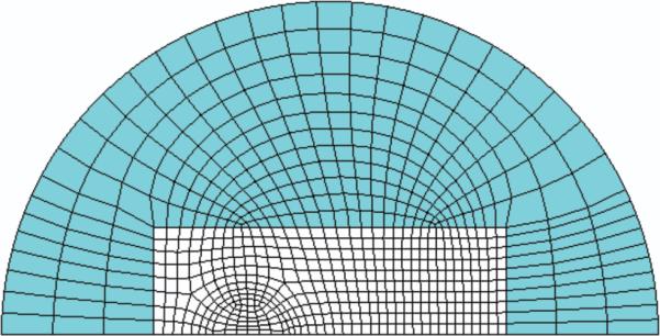
Representative axisymmetric finite element model of the VA experiment showing the coupled solid (white) and fluid (shaded) domains
Table 1.
Material properties for the model of the VA experiment
| Material | Gs (MPa) | Gl (MPa) | Bs (MPa) | Bl (MPa) | k (mm−1) |
|---|---|---|---|---|---|
| Rubber | 0.27 | 0.029 | 6.7 | 0.71 | (7.6 − 0.40i) |
| Gel | 0.13 | 0.034 | 3.2 | 0.84 | (11 − 1.4i) |
The geometry and method of excitation of the solid for this experiment will not create one specific waveform as in the first example, but rather a general (i.e. combination of modes) vibration response. However, there will continue to be a shear component of the waveform in the solid that is expected to govern the computational expense of the analysis (particularly for the softer gel material) with respect to both the solid and acoustic behavior. For the parameters given, the number of shear oscillations possible in the axial direction of the gel is approximately 130.
To perform a mesh convergence study for the simulation of the experiment with each element type, first an arbitrarily small element size was chosen (note: the mesh is necessarily unstructured to accommodate the given geometry, and therefore, element size is approximate) and an analysis was performed. Next, the mesh size was reduced by approximately 25%, an analysis was performed again, and the relative L2 – norm of the difference between the two consecutive analyses was calculated. The mesh size was reduced again and the process was repeated until the relative difference norm of two consecutive analyses was below 1%. Lastly, to compare the convergence process and computational cost of the element types, the error measure defined by Eq. (15) was calculated for each mesh size with the most refined (i.e. converged) mesh taken as the analytical solution field in the equation, and then compared to the number of DOFs.
Due to the relatively high frequency and low stiffness (resulting in the high shear wave number) for this example, traditional (i.e. low-order) elements were not able to reach convergence with the given workstation. Furthermore, rather than performing an exhaustive study of element types, as was the case for the first example, only the elements found as top performers in the first example for the given wave number range were considered. Therefore, Fig. 6 shows the convergence analysis for 7th and 9th-order elements. Clearly, both element orders were able to reach a satisfactory level of accuracy. In addition, both element types displayed monotonic convergence and appear to have reached the asymptotic error range, which supports the results of the first example that show a consistent similarity in error versus number of DOFs for the 7th and 9th-order elements. However, since the 9th-order elements have a significantly higher assembly cost (also shown in the first example) and the number of DOFs are comparable, the 7th-order elements are considerably less computationally expensive for the current problem.
Figure 6.
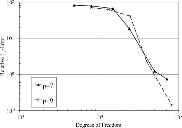
Relative L2 – error versus degrees of freedom for the mesh convergence study of the model of the VA experiment with each element type
5. Conclusions
A simple and practical approach of applying high-order spectral finite elements to alleviate the computational cost of the numerical solutions of the Helmholtz-type equations for the steady-state vibration of soft solids at high frequencies was presented. In general, high-order spectral elements were shown to be simple, in that the classical finite element formulation remains unchanged, yet effective, in that increasing element order counteracts the additional error (i.e. pollution effect) due to high wave number. Through a numerical study of a shear plane wave problem, the comparative computational expense of spectral elements with orders 3 through 14 was determined for approximately 24, 54, and 100 domain oscillations. The increase in element order was consistently found to provide a reduction in the number of DOFs required to obtain a desired level of accuracy. However, the increase in numerical integration cost and reduction in system sparsity with increasing order was shown to negatively affect the computational cost of high-order elements. With only moderately high wave number (i.e. 24 oscillations) element order around 5 was shown to be optimal for computing cost, whereas when the wave number increased orders of around 7 or 9 were shown to be more effective. A practical example was then presented representing a real experiment involving tissue phantoms and a medical imaging device. This second example showed the distinct capabilities provided by the use of 7th and 9th-order spectral elements to obtain a converged finite element model of the real system that would otherwise be unattainable through conventional (low-order) elements on a typical shared memory system.
Acknowledgements
W. Aquino and M. Aguilo would like to acknowledge the support provided by The National Institute of Biomedical Imaging and Bioengineering, Award No. EB2002167-17
Footnotes
Publisher's Disclaimer: This is a PDF file of an unedited manuscript that has been accepted for publication. As a service to our customers we are providing this early version of the manuscript. The manuscript will undergo copyediting, typesetting, and review of the resulting proof before it is published in its final citable form. Please note that during the production process errors may be discovered which could affect the content, and all legal disclaimers that apply to the journal pertain.
References
- [1].Sinkus R, Lorenzen J, Schrader D, Lorenzen M, Dargatz M, Holz D. High-resolution tensor mr elastography for breast tumour detection. Physics in Medicine and Biology. 2000;45:1649–1664. doi: 10.1088/0031-9155/45/6/317. [DOI] [PubMed] [Google Scholar]
- [2].Xydeas T, Siegmann K, Sinkus R, Krainick-Strobel U, Miller S, Claussen CD. Magnetic resonance elastography of the breast - correlation of signal intensity data with viscoelastic properties. Investigative Radiology. 2005;40:412–420. doi: 10.1097/01.rli.0000166940.72971.4a. [DOI] [PubMed] [Google Scholar]
- [3].Fatemi M, Greenleaf JF. Ultrasound-stimulated vibro-acoustic spectrography. Science. 1998;280:82–85. doi: 10.1126/science.280.5360.82. [DOI] [PubMed] [Google Scholar]
- [4].Fatemi M, Manduca A, Greenleaf JF. Imaging elastic properties of biological tissues by low-frequency harmonic vibration. Proceedings of the Ieee. 2003;91:1503–1519. [Google Scholar]
- [5].Fatemi M, Greenleaf JF. Probing the dynamics of tissue at low frequencies with the radiation force of ultrasound. Physics in Medicine and Biology. 2000;45:1449–1464. doi: 10.1088/0031-9155/45/6/304. [DOI] [PubMed] [Google Scholar]
- [6].Nightingale K, Bentley R, Trahey G. Observations of tissue response to acoustic radiation force: Opportunities for imaging. Ultrasonic Imaging. 2002;24:129–138. doi: 10.1177/016173460202400301. [DOI] [PubMed] [Google Scholar]
- [7].Alizad A, Wold LE, Greenleaf JF, Fatemi M. Imaging mass lesions by vibro-acoustography: Modeling and experiments. Ieee Transactions on Medical Imaging. 2004;23:1087–1093. doi: 10.1109/TMI.2004.828674. [DOI] [PubMed] [Google Scholar]
- [8].Alizad A, Whaley DH, Greenleaf JF, Fatemi M. Potential applications of vibro-acoustography in breast imaging. Technology in Cancer Research and Treatment. 2005;4:151–157. doi: 10.1177/153303460500400204. [DOI] [PubMed] [Google Scholar]
- [9].Ihlenburg F, Babuska I. Finite-element solution of the helmholtz-equation with high wave-number .1. the h-version of the fem. Computers and Mathematics with Applications. 1995;30:9–37. [Google Scholar]
- [10].Ihlenburg F, Babuska I. Finite element solution of the helmholtz equation with high wave number .2. the h-p version of the fem. Siam Journal on Numerical Analysis. 1997;34:315–358. [Google Scholar]
- [11].Oberai AA, Pinsky PM. A numerical comparison of finite element methods for the helmholtz equation. Journal of Computational Acoustics. 2000;8:211–221. [Google Scholar]
- [12].Oberai AA, Pinsky PM. A residual-based finite element method for the helmholtz equation. International Journal for Numerical Methods in Engineering. 2000;49:399–419. [Google Scholar]
- [13].Oberai AA, Pinsky PM. A multiscale finite element method for the helmholtz equation. Computer Methods in Applied Mechanics and Engineering. 1998;154:281–297. [Google Scholar]
- [14].Thompson LL, Pinsky PM. A galerkin least-squares finite-element method for the 2-dimensional helmholtz-equation. International Journal for Numerical Methods in Engineering. 1995;38:371–397. [Google Scholar]
- [15].Strouboulis T, Babuska I, Hidajat R. The generalized finite element method for helmholtz equation: Theory, computation, and open problems. Computer Methods in Applied Mechanics and Engineering. 2006;195:4711–4731. [Google Scholar]
- [16].Surana KS, Reddy JN. Galerkin and least-squares finite element processes for 2-d helmholtz equation in h, p, k framework. International Journal for Computational Methods in Engineering Science and Mechanics. 2007;8:1550–2295. [Google Scholar]
- [17].Deville MO, Fischer PF, Mund EH. High Order Methods for Incompressible Fluid Flow. Cambridge University Press; Cambridge: 2002. [Google Scholar]
- [18].Boyd JP. Chebyshev and Fourier Spectral Methods. 2nd edition Dover, Mineola; New York: 2001. [Google Scholar]
- [19].Vos PEJ, Sherwin SJ, Kirby RM. From h to p efficiently: Implementing finite and spectral/hp element methods to achieve optimal performance for low- and high-order discretisations. Journal of Computational Physics. 2010;229:5161–5181. [Google Scholar]
- [20].Ozgokmen TM, Iliescu T, Fischer PF. Large eddy simulation of stratified mixing in a three-dimensional lock-exchange system. Ocean Modelling. 2009;26:134–155. [Google Scholar]
- [21].Engsig-Karup AP, Hesthaven JS, Bingham HB, Madsen PA. Nodal dg-fem solution of high-order boussinesq-type equations. Journal of Engineering Mathematics. 2006;56:351–370. [Google Scholar]
- [22].Giraldo FX, Rosmond TE. A scalable spectral element eulerian atmospheric model (see-am) for nwp: Dynamical core tests. Monthly Weather Review. 2004;132:133–153. [Google Scholar]
- [23].Iskandarani M, Haidvogel DB, Levin JC. A three-dimensional spectral element model for the solution of the hydrostatic primitive equations. Journal of Computational Physics. 2003;186:397–425. [Google Scholar]
- [24].Komatitsch D, Tromp J. Introduction to the spectral element method for three-dimensional seismic wave propagation. Geophysical Journal International. 1999;139:806–822. [Google Scholar]
- [25].Hesthaven JS, Warburton T. High-order accurate methods for time-domain electromagnetics. Cmes-Computer Modeling in Engineering and Sciences. 2004;5:395–407. [Google Scholar]
- [26].Graff KF. Wave Motion in Elastic Solids. Dover Publications, Inc.; New York: 1975. [Google Scholar]
- [27].Solin P. Partial Differential Equations and the Finite Element Method. John Wiley and Sons, Inc.; Hoboken, New Jersey: 2006. [Google Scholar]
- [28].Cook RD, Malkus DS, Plesha ME, Witt RJ. Concepts and Applications of Finite Element Analysis. 4th edition Wiley; 2001. [Google Scholar]
- [29].Urban MW, Kinnick RR, Greenleaf JF. Measuring the phase of vibration of spheres in a viscoelastic medium as an image contrast modality. Journal of the Acoustical Society of America. 2005;118:3465–3472. doi: 10.1121/1.2130947. [DOI] [PubMed] [Google Scholar]
- [30].Brigham JC, Aquino W, Mitri FG, Greenleaf JF, Fatemi M. Inverse estimation of viscoelastic material properties for solids immersed in fluids using vibroacoustic techniques. Journal of Applied Physics. 2007;101:23509-1–14. [Google Scholar]
- [31].Findley WN, Lai JS, Onaran K. Creep and Relaxation of Nonlinear Viscoelastic Materials. Dover; 1989. [Google Scholar]