Dynamic frame selection for in vivo ultrasound temperature estimation during radiofrequency ablation

Abstract

Minimally invasive therapies such as radiofrequency ablation have been developed to treat cancers of the liver, prostate and kidney without invasive surgery. Prior work has demonstrated that ultrasound echo shifts due to temperature changes can be utilized to track the temperature distribution in real time. In this paper, a motion compensation algorithm is evaluated to reduce the impact of cardiac and respiratory motion on ultrasound-based temperature tracking methods. The algorithm dynamically selects the next suitable frame given a start frame (selected during the exhale or expiration phase where extraneous motion is reduced), enabling optimization of the computational time in addition to reducing displacement noise artifacts incurred with the estimation of smaller frame-to-frame displacements at the full frame rate. A region of interest that does not undergo ablation is selected in the first frame and the algorithm searches through subsequent frames to find a similarly located region of interest in subsequent frames, with a high value of the mean normalized cross-correlation coefficient value. In conjunction with dynamic frame selection, two different two-dimensional displacement estimation algorithms namely a block matching and multilevel cross-correlation are compared. The multi-level cross-correlation method incorporates tracking of the lateral tissue expansion in addition to the axial deformation to improve the estimation performance. Our results demonstrate the ability of the proposed motion compensation using dynamic frame selection in conjunction with the two-dimensional multilevel cross-correlation to track the temperature distribution.

Introduction

Minimally invasive therapies have gained increasing attention in the last decade as an alternative to standard surgical therapy (Hill and ter Haar 1995, Murphy and Gill 2001, Chin and Pautler 2002, Goldberg and Ahmed 2002, Ogan and Cadeddu 2002, Tunuguntla and Evans 2002). They are being investigated for the treatment of many diseases such as primary hepatocellular carcinoma (HCC) (Goldberg 2001, Haemmerich et al 2001, Goldberg and Ahmed 2002), lower urinary tract symptoms due to benign prostatic hyperplasia (Goldberg et al 1998, Beerlage et al 2000, Tunuguntla and Evans 2002) and small renal-cell carcinoma (RCC) (Gervais et al 2000, Murphy and Gill 2001, Chin and Pautler 2002, Ogan and Cadeddu 2002). Temperatures greater than 42 °C are considered potentially lethal, depending on the duration of application (Rosner et al 1996), and temperatures greater than 60 °C are associated with uniform tissue necrosis. Benefits over surgical resection include the anticipated reduction in morbidity and mortality, lower cost, suitability for real-time image guidance, ability to perform ablative procedures on outpatients and the potential applicability to a wider spectrum of patients, including nonsurgical candidates.

The trend toward minimally invasive options in the management of renal tumors has also prompted interest in ablation techniques as possible alternatives to radical or partial nephrectomy (Savage and Gill 2000, Johnson and Nakada 2001, Murphy and Gill 2001). Laparoscopic renal cryoablation, RF, microwave and HIFU ablative therapies are some of the modalities used for renal tumors (Savage and Gill 2000, Johnson and Nakada 2001, Murphy and Gill 2001). RF ablation employs needle electrodes placed percutaneously and directly through open surgery into renal lesions. In the United States, only RF and cryoablation are approved by the U.S. Food and Drug Administration (FDA) for treating RCC (Goldberg et al 2000, Mirza et al 2001, Murphy and Gill 2001, Chin and Pautler 2002, Ogan and Cadeddu 2002).

Currently the positioning of the RF ablation electrode into the tumor site is done under ultrasound guidance. However, Gazelle et al report that the ablated region can appear to be hyper-echoic, hypo-echoic or have the same echogenicity as the ablation site prior to treatment (Gazelle et al 2000). This has led to the examination of a range of ultrasound parameters to determine their efficacy in providing real-time temperature maps during RF ablation. These approaches include tracking tissue acoustic properties (Ueno et al 1990, Maass-Moreno et al 1996, Seip et al 1996, Simon et al 1998, Sun and Ying 1999, Varghese et al 2002), attenuation (Ueno et al 1990, Worthington and Sherar 2001, Clarke et al 2003, Techavipoo et al 2004), backscatter changes (Straube and Arthur 1994, Arthur et al 2005), tracking frequency shifts of the center frequency and its harmonics (Palussiere et al 2003), and tracking timeshifts in the ultrasound echo signal introduced due to the speed of sound changes (Nasoni 1981), thermal expansion without (Seip and Ebbini 1995) and with the speed of sound changes with temperature (Simon et al 1998, Varghese et al 2002, Varghese and Daniels 2004, Techavipoo et al 2005, Daniels et al 2007, Anand and Kaczkowski 2008, Daniels 2008, Daniels et al 2008). Tracking the shift in the ultrasound echo signal due to thermal expansion and speed of sound changes is the only method that has been demonstrated to track temperature changes in the range from 40 °C to 100 °C generally observed during RF ablation procedures (Varghese et al 2002). It should also be noted that RF ablation has been monitored utilizing MRI for the liver (Seror et al 2006).

The focus of this paper is on imaging the temperature distribution produced during RF ablation procedures utilizing the shift in the ultrasound echo signal due to thermal expansion and speed of sound changes. This type of ultrasound-based method relies on the ability to accurately track small frame-to-frame displacements due to the movement of tissue scatterers associated with the temperature increase. These displacements are then accumulated over the duration of the ablation procedure, and the gradient of the displacement related to the temperature change utilizing a calibration curve (Varghese and Daniels 2004). Previous works by Daniels et al (2007, 2008) have demonstrated that this method of ultrasound-based temperature imaging of RF ablation is feasible using both realistic finite element analysis (FEA)/ultrasound simulations and tissue-mimicking phantom experiments.

However, in each of the prior experiments (Daniels et al 2007, 2008), there were no associated external motion artifacts that could lead to errors in the displacement estimation. Clinically, there are two primary types of motion (cardiac and respiratory) that would affect the temperature map. Respiratory motion constitutes the largest source of error in the displacement estimates (Chandrasekhar et al 2006). This is due to the fact that scatterers that contribute to the ultrasound speckle signature that are in the ultrasound scan plane at the beginning of the respiratory cycle may not be in the same scan plane a few frames later due to the elevational motion causing speckle tracking methods such as one-dimensional (1D) and 2D cross-correlation to fail to track these displacements (Chandrasekhar et al 2006). Cardiac motion on the other hand does not result in significant elevational motion and therefore is considered a secondary effect when compared to respiratory motion in our analysis (Chandrasekhar et al 2006).

Since motion due to the cardiac and respiratory cycles can cause significant errors in ultrasound-based temperature maps, a method needs to be developed to compensate for these types of motion artifacts (Chandrasekhar et al 2006). Several different types of motion compensation have been successfully used with ultrasound to date such as manually translating the B-mode images (Mokhtari-Dizaji et al 2006) or using an ultrasound transducer to track the motion of the diaphragm throughout the respiratory cycle to provide motion compensation for catheter navigation through blood vessels (Timinger et al 2005). Ultrasound-based methods of motion compensation have also found that mutual information was more computationally intensive and sensitive to noise than the cross-correlation coefficient method (Xu and Hamilton 2006).

This paper provides a description of an in vivo RF ablation experiment on porcine kidneys and the tracking of resulting displacements and temperature changes. A novel method is proposed to track displacements utilizing dynamic frame selection and only tracking displacements between frames with a high mean normalized cross-correlation coefficient. A comparison of the efficacy of two cross-correlation algorithms, 2D CC and a novel 2D multilevel cross-correlation algorithm developed by Shi and Varghese (2007) in determining local displacements and temperature maps, is also made.

Materials and Method

In vivo RF ablation under ultrasound guidance was performed on porcine kidneys for duration of 8 min using a Radionics (now Valley Lab, Boulder, CO) Cool-Tip RF system (Radionics, Burlington, MA) and the Ultrasonix 500RP clinical ultrasound system (Ultrasonix Medical Corporation, Vancouver, BC, Canada). The Cool-Tip RF system electrode circulates chilled water internally which cools the tissue immediately surrounding the electrode and reduces the effects of tissue charring around the electrode (Valleylab 2007). The Radionics system also contains a feedback mechanism that monitors the tissue temperature around the electrode with a thermocouple and adjusts the radiofrequency energy to minimize tissue charring. Due to the circulation of the chilled water, the Radionics system does not provide real-time temperature estimates.

Two pigs (mean weight = 40 kg) were used in this study. The study was conducted under a protocol approved by the Research Animal Care and Use Committee of the University of Wisconsin-Madison. Anesthesia was induced using intramuscular tiletamine hydrochloride and zolazepam hydrochloride (Telazol; Fort Dodge, IA), atropine (Phoenix Pharmaceutical, St Joseph, MO) and xylazine hydrochloride (Xyla-Ject; Phoenix Pharmaceutical, St Joseph, MO). Animals were intubated and anesthesia maintained with inhaled isoflurane (Halocarbon Laboratories, River Edge, NJ). The pigs were placed in a supine position and prepared in the midline and draped. Through a midline incision, one kidney was dissected free, and the lower pole exposed. An identical procedure was performed on the contralateral side for the other kidney. Approximately 1–2 cm of respiratory induced motion was observed in the kidneys during the ablation procedure. Depending on the location of the tumor, either open surgery or the less invasive percutaneous ablation is performed. The open surgical method was examined in these experiments due to the method allowing us to accurately position the ultrasound probe over the RF ablation needle.

RF ablation was performed on the lower pole of the kidney with the needle advanced under ultrasound guidance. The ultrasound transducer was placed on the kidney and adjusted to ensure that the RF ablation needle was visible in the ultrasound scan plane as shown in figure 1. An acoustically transparent gelatin pad was placed between the transducer and the kidney to ensure good acoustic coupling. In addition, the gelatin pad ensured that no damage occurred to the transducer due to heat transfer from the kidney during the ablation procedure. The kidney was positioned in order to ensure good contact between the gelatin pad and the kidney for the duration of the ablation procedure. The ablation procedure was performed on both the right and left kidneys in each animal, with two ultrasound RF echo data sets collected per animal.

Figure 1.

Schematic diagram indicating the placement of the RF electrode and ultrasound transducer, into a kidney.

Following treatment, the kidneys were allowed to cool to body temperature and the visible lesion evaluated and the kidney replaced in situ. The pigs were allowed to survive for 48 h to better evaluate cell death and then euthanized as per the University of Wisconsin-Madison’s animal care guidelines. Forty-eight hours allowed coagulative necrosis to be clearly identified. The kidneys were harvested and fixed in a 10% formalin solution. The kidney was then sliced along the ultrasound scan plane to obtain pathological visualization of the treated region.

RF echo data acquisition

Ultrasound radiofrequency echo data were acquired at a frame rate of 2 frames per second using the Ultrasonix 500RP system equipped with a research interface after beam forming. This frame rate was selected as a compromise to enable the collection of data at a sufficient frame rate for temperature imaging coupled with the storage of the data on the system to ensure real-time data acquisition. A 1D linear array ultrasound transducer with a 6.6 MHz center frequency and 40 mm imaging width was used. The transducer was held in a fixture attached to the table on which the animal was placed. The ultrasound transducer has an approximate 60% bandwidth and the echo signals were digitized using a 40 MHz sampling frequency. The research interface on the ultrasound system recorded radiofrequency echo signal frames every 0.5 s as the porcine kidneys underwent an 8 min RF ablation procedure. The transducer provided echo signals over an area of 5 cm (width) by 3–5 cm depth (depending on the thickness of the kidney). The Cool-Tip RF probe keeps the maximum temperature in the tissue at or less than 99 °C by monitoring the tissues’ temperature with an embedded thermocouple.

Dynamic frame selection

Dynamic frame selection in this paper was utilized as a motion compensation algorithm both to minimize extraneous motion artifacts and to optimize computational costs by reducing the number of radiofrequency data frames processed. In previous papers (Daniels et al 2007, 2008), the authors reported on methods where displacement estimates were accumulated at set intervals, e.g. the displacement between frames 0 and 6 was accumulated, then the displacement between frames 6 and 12, and so on. This strategy can lead to errors in accumulating the displacement if objects within the ultrasound scan plane are not in the same location during frame 0, 6 and 12. Movement of tissue within the ultrasound scan plane due to elevational motion from respiration has to be accounted for displacement estimation especially under in vivo imaging conditions. If the imaged tissue is not in the same location, echo signals from frames (for e.g. 0 and 6) will be highly decorrelated due to the presence of completely different scattering in each frame (Techavipoo et al 2005).

One of the solutions to mitigate this problem would be to acquire data at higher frame rates, faster than the rate at which scatterers move out of the ultrasound scan plane due to respiratory or cardiac motion. Hence, by accumulating the displacement every few frames the effects of elevational motion should be minimized since the same structures would exist in each RF echo frame. However, if the displacement between frames is accumulated at high frame rates when the displacement between frames is small, accumulation of the displacements also lead to accumulation of noise artifacts associated with the displacement estimate. These noise artifacts accumulate at a faster rate for higher frame rates as opposed to frame rates that provide adequate tracking of larger displacements albeit at a lower frame rate.

The method proposed in this paper attempts to address both these issues associated with errors in displacement estimates due to elevational motion and the accumulation of frame-to-frame displacements at higher frame rates. By appropriately choosing a start frame and dynamically choosing the next frame for processing in order to accumulate the displacement, the errors due to the above-mentioned challenges are minimized. A small region of interest (ROI) is chosen on the start frame in a region that does not undergo ablation. The mean normalized cross-correlation coefficient in this ROI between the start frame and all other frames throughout the respiratory cycle is then calculated after skipping the first few frames immediately following the start frame. For example, the cross-correlation coefficient will be calculated between frames 0 and frames 20–120 if the frame rate is 30 fps and the respiratory cycle is approximately 3 s.

Once all of the mean normalized cross-correlation coefficients for the ROI are calculated, the frame-to-frame displacement is calculated between the start frame and the frame that had the highest mean normalized cross-correlation coefficient. The second frame then becomes the start frame and is utilized to estimate the next matching frame for displacement estimation. This procedure is then repeated using the frame with the highest mean normalized cross-correlation coefficient as the next start frame and so on. This allows the frame-to-frame displacement to be calculated while minimizing the impact of external motion due to respiratory and cardiac sources. In addition, the resulting frame-to-frame displacement is not prone to errors due to small frame-to-frame local displacements due to the larger separation between frames. In addition, since the technique is dynamic it will adjust based on the frame chosen even if the respiratory cycle duration of the patient changes during the procedure.

Displacement estimation

Once the dynamic frame selection algorithm has been used to identify the radiofrequency frames that are highly correlated, an estimate of the local displacement between consecutive frames is calculated. Both actual (due to thermal expansion) and virtual (due to sound speed variations) shifts in the echo signal contribute to this displacement. A 2D multi-level cross-correlation and a 2D block matching method are then utilized to track these local displacements. Displacement estimates are obtained by estimating the location of the sub-sample peak of the cross-correlation function of the pre- and post-deformation echo signals. The 2D block matching method is based on a predictive search algorithm that utilizes the prior displacement estimate along the axial direction to predict the current displacement estimate. The 2D block matching method also checks for consistency between displacement estimates before moving from one search row to the next.

The 2D multi-level cross-correlation method was developed to compute local displacement fields and strains in discontinuous media (Shi and Varghese 2007). Coarse displacement estimates are initially obtained using sub-sampled B-mode data using a multilevel pyramid algorithm. The coarse displacement estimates are then utilized to guide the high resolution estimation on the lowest level of the pyramid containing the radiofrequency echo signal data. This method combines advantages provided by the robustness of B-mode envelope tracking and the precision obtained using RF motion tracking to obtain high resolution displacement and strain estimates. The design of this method utilizing the multi-level pyramid algorithm also incorporates lateral motion compensation between frames (for motion within the imaging plane) since this search algorithm maximizes the correlation coefficient by appropriately positioning the kernel in the post-deformation radiofrequency data frame.

Temperature estimation

After the displacement is estimated between frames, the gradient of the cumulative displacement was computed and the displacement gradient versus temperature calibration curve (Techavipoo et al 2005) was used to convert the gradient value to a temperature estimate (Varghese et al 2002). The displacement gradient versus temperature calibration curve was calculated based on experimental ex vivo measurements of the thermal expansion and the speed of sound changes with temperature of tissue. These parameters are required a priori and have to be determined for each tissue type undergoing ablation. The change in temperature to the gradient of the displacement are related from the expression G= (c₀/c)(δ + 1) − 1, where δd represents the normalized tissue expansion given by $\delta d=\frac{d_0-d}{d_0}$, c denotes the speed of sound of tissue at the elevated temperature, c₀ is the speed of sound at 37 °C, d₀ is the initial distance between two points in tissue and d is the distance between two the points in tissue at the elevated temperature. This creates a single-valued curve that relates the displacement gradient (G) to temperature (Techavipoo et al 2005). The curve is valid for a temperature range of 37–100 °C. A lookup table is utilized to transform the gradient of the displacement to a temperature estimate. The same parameters were used to obtain the displacement gradient for both the 2D block matching and 2D multi-level cross-correlation algorithms.

Results

Figure 2(a) depicts a B-mode image of a porcine kidney ablation procedure after 30 s of ablation. The dark region at the top of figure 2(a) is due to the acoustically transparent gelatin pad. Note the line of scattering from approximately 4–6 cm down and 2.75 cm across. This increase in the scattering represents reverberations from the tip of the RF ablation needle, which is placed approximately 3 cm below and 2.75 cm across and within the scanning plane. The hyper-echoic region across the width of the figure at a depth ranging from 4.5 cm to 5 cm represents the kidney (above) and soft tissue (below) interface.

Figure 2.

B-mode image after 30 s of ablation (a), along with the displacement map during a porcine kidney ablation procedure using (b) 2D block matching and (c) multi-level 2D cross-correlation after 30 s of ablation. The corresponding temperature maps after 30 s of ablation using the two algorithms are shown in (d) and (e).

Figures 2(b) and (c) present displacement maps computed using 2D block matching (figure 2(b)) and the multi-level 2D cross-correlation (figure 2(c)) method, respectively. Note that the general pattern of the displacement observed is similar in both figures 2(b) and (c). However, in figure 2(b), the maximum displacement is 0.3 mm and the minimum displacement is −0.4 mm. This is slightly different than that in figure 2(c), where the maximum displacement is 0.35 mm and the minimum displacement is −0.2 mm.

Figures 2(d) and (e) present temperature maps based on the displacement maps in figures 2(b) and (c), respectively. The thermal expansion curves obtained for kidney specimens are very similar to the expansion curves observed with liver specimens (Varghese and Daniels 2004). Note that while figure 2(d) suggests a maximum temperature of 100 °C, the maximum temperature in figure 2(e) is only 75 °C. This is due to the fact that displacement estimates in figure 2(b) have larger gradients along an A-line than those found in figure 2(c). The exact temperature increase versus time has not been measured for the Radionics RF ablation system. However, it is known that the Radionics RF ablation system does not reach a maximum temperature of 100 °C for at least 60 s (Valleylab 2007).

The B-mode image after 4 min of ablation is presented in figure 3(a). Note the hyper-echoic area in the center of the image, which is also the center of the ablated area, due to gas bubbles forming from the out-gassing of the water vapor which generally occurs as the temperature in the kidney is approximately 100 °C. It should also be noted that the hyper-echoic region is centered on the location of the RF ablation electrode in figure 2(a). In addition, note that the hyper-echoic line that forms the boundary between the kidney and gelatin interface has moved toward the surface of the transducer due to thermal expansion and the speed of sound changes. For instance at a width of 2.5 cm, the interface has moved from a depth of 0.5 cm after 30 s of ablation to a depth of 0.25 cm after 4 min of ablation. In a similar fashion, the hyperechoic line that forms the kidney and soft tissue interface has moved away from the transducer and has moved from a depth of 4.5 cm to 5 cm or lies outside the ultrasound scan plane between 2 and 3 cm along the x-axis.

Figure 3.

B-mode image after 4 min of ablation (a), along with the displacement map during a porcine kidney ablation procedure using (b) 2D block matching and (c) multi-level 2D cross-correlation. The corresponding temperature maps after 4 min of ablation using the two algorithms are shown in (d) and (e).

Notice also the presence of streak artifacts in the displacement estimate after 4 min of ablation (figure 3(b)). These streak artifacts are due to 2D block matching using a predictive method for displacement estimation. The predictive method works by predicting a displacement estimate at the position x along an A-line from the displacement estimate at the position x − 1 along the same A-line. Thus, if 2D block matching severely over or underestimates the displacement estimated along an A-line, it can cause all further displacement estimates along that A-line to become skewed. This is why the displacement estimates appear to be continuous at the top of the displacement map in figure 3(b) but not at the bottom. The displacement estimate obtained using multi-level 2D cross-correlation after 4 min of ablation as shown in figure 3(c) does not include the streak artifacts shown in figure 3(b).

Temperature maps after 4 min of ablation are presented for the 2D block matching and multi-level 2D cross-correlation in figures 3(d) and (e), respectively. Note that both temperature maps suggest a maximum temperature of 100 °C. The temperature map in figure 3(d) is significantly noisier than the temperature map in figure 3(e). This is due to the significantly lower level of noise in figure 3(c) as compared to figure 3(b). In addition, the area that corresponds to an estimated temperature of 100 °C in figure 3(e) matches with the hyper-echoic region in figure 3(a).

Finally, figure 4(a) presents a B-mode image of the porcine kidney tissue after 8 min of ablation, the maximum duration of the RF ablation procedure. The hyper-echoic region in the center of the figure 4(a) has also increased in dimension with respect to figure 3(a), due to the continued ablation of the region. The displacement map with 2D block matching is presented in figure 4(b), and the multi-level 2D cross-correlation displacement map is presented in figure 4(c). Similar to the results presented in figures 3(b), the results in 4(b) indicate multiple streak artifacts along A-lines due to the incorrect estimation of displacements along that A-line. This is demonstrated in figure 4(b), where the streak artifacts are more prevalent than in the previous figure 3(b). In the figure that utilizes multi-level 2D cross-correlation (figure 4(c)), the streak artifacts are not visualized after 8 min of ablation. Hence, multi-level 2D cross-correlation is able to accurately track displacements after 8 min of ablation, while 2D block matching suffers from streak artifacts due to incorrect displacement estimation.

Figure 4.

B-mode image after 8 min of ablation (a), along with the displacement map during a porcine kidney ablation procedure using (b) 2D block matching and (c) multi-level 2D cross-correlation. The corresponding temperature maps after 8 min of ablation using the two algorithms are shown in (d) and (e).

The increased presence of streak artifacts in figure 4(b) compared to figure 3(b) contributes to a temperature map in figure 4(d) that is significantly noisier than that shown in figure 3(d). Although the central ablated region suggests a value of 100 °C, as does much of the area outside the hyper-echoic region in figure 4(a), it is difficult to determine the area being ablated in figure 4(d). Due to the fact that figure 4(c) does not suffer from the same type of streak artifacts, the ablated region is easily visualized in figure 4(d). Note that the size of the ablated region has increased as compared to figure 3(d). This is similar to the increase in the size of the hyper-echoic region in figure 4(a) as compared to figure 3(a).

A graph of the mean normalized cross-correlation coefficient versus time for the porcine kidney ablation procedure is presented in figure 5. The mean normalized cross-correlation coefficient was calculated by finding the mean cross-correlation coefficient between each pair of start and end frames over the ROI that was used to estimate the displacement and temperature maps. Figure 5 shows that the mean normalized cross-correlation coefficient never drops below 0.4. Hence, by using dynamic frame selection, frames that are uncorrelated with the start frame are not used to track the frame-to-frame displacements, with the overall average cross-correlation coefficient over 0.66 for all pairs of start and end frames.

Figure 5.

Plot of the mean normalized cross-correlation coefficient versus time for the porcine kidney ablation shown in figures 2–4.

Figure 6 presents results obtained for a second in vivo porcine kidney ablation procedure. In figure 6, each row represents different ablation durations namely 30 s (row I), 4 min (row II), 6 min (row III) and 8 min (row IV), respectively. In each row the corresponding B-mode image (a), displacement map (b) and temperature map (c) obtained using only the 2D multi-level cross-correlation method are presented. Block matching results are not presented in the rest of this paper, due to the increased streak noise artifacts with this method.

Figure 6.

B-mode (a), displacement (b) and temperature (c) map obtained using the multi-level 2D cross-correlation after (I) 30 s, (II) 4 min, (III) 6 min and (IV) 8 min during an RF ablation procedure on a in vivo porcine kidney.

In figure 6(a), row I, note that the kidney-acoustic gel interface is visible at the top of the image and the kidney-soft tissue interface is visible along the left side and bottom of the B-mode image at a depth of 3 cm for a width of 1 cm and a depth of 4.25 cm for a width of 5 cm. Note that the maximum estimated temperature after 30 s of ablation in figure 6(c), row I (~70 °C) is similar in magnitude to the maximum temperature after 30 s of ablation in figure 2(c) (~75 °C). The B-mode image and displacement and temperature maps after 4 min of ablation are presented in row II. Note that the kidney-acoustic gel boundary in figure 6(a), row II, has moved toward the transducer, and the kidney-soft tissue boundary at the bottom of the image has moved away from the transducer as compared to figure 6(a), row I, from a depth of 0.25 cm along the center of the image to a depth of 0.1 cm. In addition, the kidney-soft tissue interface on the left of the image has moved toward the right as compared to figure 6(a) from a width of 0.5 cm to a width of 1 cm. This is due to external motion of the kidney relative to the transducer. Due to this shift there is a hypo-echoic region on the left of the image where there is no longer good contact between the acoustic gel pad and the soft tissue to the left of the kidney.

In figure 6(b), row II, the magnitude of the maximum and minimum displacement has increased when compared to figure 6(b), row I, due to thermal expansion. Note that the displacement is negative (toward the transducer) at the top of the displacement map and positive (away from the transducer) at the bottom of the displacement map. These results are consistent with the FEA simulation results reported in Daniels et al (2008), where the displacements were negative above the RF ablation needle and positive posterior to the RF ablation needle. The temperature map in figure 6(b), row II, is similar to the temperature map in figure 3(e) in that both temperature maps suggest a maximum temperature of 100 °C after 4 min of ablation. In addition, the high temperature region 2 cm deep and 3 cm across corresponds to the location of the RF ablation needle. Hence, after 4 min of ablation the multi-level 2D cross-correlation is able to track the location of the ablated region for different in vivo kidney ablation experiments.

In figure 6, row III presents the corresponding B-mode image, displacement and temperature map after 6 min of ablation. In figure 6(b), row III, note that the magnitude of the maximum and minimum displacements has increased as compared to figure 6(b), row II as expected. In addition, the overall shape of the displacement maps is similar in both images. In figure 6(c), row III, the size of the region estimated at 100 °C has increased when compared to figure 6(c), row II. This is also as expected since the size of the ablated region should increase during the ablation procedure. The final row in figure 6, row IV, presents the corresponding B-mode, displacement and temperature maps after 8 min of ablation. There is no significant difference between the B-mode image presented in row IV and that found in row III.

The overall average cross-correlation coefficient between all pairs of start and end frames for the ROI used to calculate the displacement and temperature maps in figure 6 was around 0.71. This is slightly higher but not significantly different than the average cross-correlation coefficient of 0.66 shown in figure 5.

A region of interest (ROI) was selected near the center of the ablated region as depicted in figure 7(a). From this ROI, a time versus estimated temperature graph was calculated and is shown in figure 7(b). Note the fairly steady increase in estimated temperature over time until the temperature estimate is approximately 100 °C at three and a half minutes. The temperature estimated remains near 100 °C for the duration of the ablation procedure.

Figure 7.

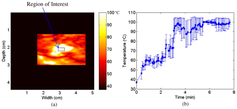
A region of interest (ROI) outlined on a temperature map in (a) along with the estimated temperature versus time graph with error bars (b) obtained for the ROI over the duration of the ablation procedure.

Pathology results for the porcine kidney ablation procedure depicted in figure 6 are shown in figure 8. The kidney was sliced into cross-sections in order to determine the size of the ablated region. The two slices shown in figure 8 are representative slices at the center of the kidney. Note that the ablated area corresponds to the darker area in the superior right region of each cross-section. The RF ablation needle track is visible on each slice below the blue lines. The scale at the bottom of the photograph provides dimensions of the ablated region.

Figure 8.

Pathology results for the porcine kidney shown in figure 6. The images presented represent sliced cross-sections of the kidney tissue following ablation. The scale provided at the bottom is utilized to measure the thermal lesion dimensions.

The blue lines on the image correspond to the length from the RF needle track to the distal edge of the kidney. For the kidney cross-section on the left, this distance is 1.8 cm, and for the kidney cross-section on the right, this distance is 1.9 cm. In figures 6(b) and (c) in rows II–IV, the edge of the kidney is at ~1 cm from the left of the image and both the locations of the maximum magnitude for the displacement and the maximum temperature are located at ~2.8 cm. The location of the RF ablation needle in the kidney is ~1.8 cm from the distal edge of the kidney. Hence, the pathology results (~1.8 cm from the distal edge of the kidney) correspond well to the location of the RF needle in figure 6 (~1.8 cm from the distal edge of the kidney).

Discussion and conclusion

Generation of temperature maps during an RF ablation procedure, necessitate tracking and estimation of frame-to-frame displacements. Clinically, there are two major sources of extraneous motion, respiratory and cardiac, that can introduce errors into the frame-to-frame displacement estimation. Of these two types of motion, respiratory motion introduces by far larger errors than cardiac motion. This is due to the fact that respiratory motion introduces elevational motion in addition to axial and lateral deformations. Cardiac motion on the other hand introduces primarily axial and lateral motion artifacts. Elevational motion due to respiration is a significant concern since scatterers along the elevational ultrasound scan plane become completely uncorrelated to scatterers in a different ultrasound scan plane. Hence, frame-to-frame displacements between scan planes (out-of-plane) are not tracked accurately with 2D displacement estimation methods. Motion in the axial and lateral direction can be tracked because the scatterers are moving within the same ultrasound scan plane.

A motion compensation algorithm was developed to dynamically select the next frame given a start frame. The algorithm was evaluated using radiofrequency data acquired from in vivo RF ablation of porcine kidneys. An ROI that does not undergo ablation is selected in the first frame and the algorithm searches through the subsequent frames to find the ROI in frames with the highest mean normalized cross-correlation coefficient with the start frame. This new frame becomes the post-compression frame and the displacement between these two frames is then calculated. The post-compression frame then becomes the new start frame and the process starts over. This allows the frame-to-frame displacement to be calculated while minimizing the effect of external motion due to respiratory and cardiac cycles.

Selection of the frames to be processed in this manner ensures that significant out-of-plane (elevational) motion would not exist between these frames. The mean normalized cross-correlation coefficient between frames will be low with larger elevational motion (during inspiration) and that frame would not be selected as the frame to be processed for displacement accumulation. The start frame is generally selected during expiration (where extraneous motion is reduced); this method would allow the subsequent frame to be selected during expiration during the next respiratory cycle even if the length of the respiratory cycle varies during the ablation procedure.

In addition, the ability of two different 2D displacement estimation methods to track frame-to-frame deformations was compared. Both methods track displacements without significant errors after 30 s of ablation (figure 2). However, the 2D block matching temperature map estimates higher temperatures (100 °C) than the multi-level 2D method (70 °C). The multi-level 2D cross-correlation results obtained were similar to the experimental results using the RITA 1500 RF ablation electrode previously used (Daniels et al 2007, 2008). After 8 min of ablation, the 2D block matching algorithm develops significant streak artifacts in its displacement map due to displacement tracking errors. These streak artifacts were due to the fact that since 2D block matching uses a predictive search algorithm, once a displacement error is made all subsequent displacement estimates along that A-line will suffer from the same error. These errors in the displacement in turn lead to errors in the temperature map seen in figure 4(d). The multi-level 2D cross-correlation algorithm results in figure 4(c), on the other hand, do not contain streak artifacts since the algorithm incorporates additional lateral motion compensation and improved localization of the data segment for signal processing. The temperature map in figure 4(e) calculated from the multi-level 2D cross-correlation displacement map corresponds well to the hyper-echoic region observed in figure 4(a). These results were corroborated with additional temperature maps obtained on independent in vivo ablation procedures in figure 6, demonstrating the improved performance with the 2D multi-level cross-correlation algorithm.

The overall mean cross-correlation coefficient values obtained were 0.66 and 0.71, respectively. In addition, an estimated temperature versus time graph was also calculated for an ROI near the center of the ablated region for the second in vivo kidney ablation. The graph demonstrates that the multi-level 2D cross-correlation algorithm is able to track the temperature change from 37 °C to 100 °C for the ROI. The graph also demonstrates that the estimated temperature remains at 100 °C for the duration of the ablation procedure.

For the in vivo RF ablation experiment in figure 6, pathological cross-sectional slices of the ablated kidney were available and are presented in figure 8. The cross-section of the kidney was utilized to compare the location of the RF ablation needle track in the displacement and temperature maps to the location of the RF ablation needle track on the cross-section. For this experiment, it was found that the location of the RF ablation needle track laterally was similar on the cross-sectional slices as on the displacement maps. The depth of RF ablation needles was unable to be determined due to the difficulty in determining the end depth of the RF ablation needle track.

The results presented in figures 2–7 demonstrate the ability of the multi-level 2D cross-correlation method to track the region undergoing in vivo RF ablation in the porcine kidney for up to 8 min. This result is significant for several reasons. First, this experiment demonstrates that displacements can be tracked in vivo in porcine kidney tissue when motion due to respiration and cardiac activity is present. Although displacement and temperatures have been successfully tracked in vivo (with increased noise artifacts) for an entire ablation procedure (Varghese et al 2002), these results indicate the successful utilization of motion compensation using both dynamic frame selection and lateral motion tracking within the scanning plane using the 2D multi-level cross-correlation method to accurately register and accumulate the displacement estimates over the entire ablation duration. In addition, some of the previous in vivo experimental results reported by other groups have successfully tracked the temperature for only the first 2 min of the ablation procedure (Varghese et al 2002) or for only limited temperature increases (Liu and Ebbini 2010). Hence, these results represent a significant advance in the ability to track displacements under in vivo conditions and temperature over the entire duration of a clinical ablation procedure.

The results presented in this paper also compare well to those obtained using the promising PRF method of MR thermometry for both RF ablation of the liver (Seror et al 2006) and HIFU ablation of the prostate (Rieke et al 2004, Pauly et al 2006, Rieke et al 2007). MR thermometry has demonstrated the ability to track temperatures greater than 60 °C over the duration of a HIFU ablation procedure (Pauly et al 2006) as well as in the prostate which can undergo large amounts of motion during treatment (Rieke et al 2007). Ultrasound-based temperature imaging does have several advantages over MR thermometry however. MRI machines are very expensive to buy and maintain. Therefore, there are only a limited number of them available in hospitals. With the increase in the projected number of RCC-related procedures in the United States over the next decade, other imaging modalities that perform temperature imaging need to be examined. Secondly, MRI-compatible RF devices are still being tested and are not widely used or available clinically. Seror et al (2006) recently reported that PRF-based temperature imaging during RF ablation of HCC is feasible with a ±4 °C uncertainty. However, to accomplish this home-made copper RF electrodes were needed to reduce the noise in MRI temperature images, as current clinical RF ablation systems introduced severe noise artifacts.

It should be noted that a major limitation of this study was the frame rate of the Ultrasonix system (2 frames s⁻¹). This was a limitation of the system due to the research interface that was being utilized. In addition, this limitation led to the invasive nature of the experimental setup in order to ensure that the respiratory and cardiac motion of the kidneys could be controlled. However, despite this limitation we were able to track displacements and temperature over an 8 min ablation procedure with limited respiratory and cardiac motion due to the experimental setup. Given that high end systems have much higher frame rates (>30 frames s⁻¹ for high end systems), this method should be able to be extended to clinical cases where greater out-of-plane motion occurs due to respiration. An example of this is the out-of plane motion that occurs during breast elastography. In breast elastography, breast tissue is manually compressed up to 20% (Hall et al 2003) against the chest wall, thereby inducing large out-of-plane motions, and has been successfully tracked by a high frame rate system.

There are several areas for future research utilizing this method of ultrasound-based temperature estimation. For instance, besides higher frame rates, another way to improve the data acquisition would be to gate the data acquisition with the high frame rates at the start of the expiration and acquire data only for the expiration duration from 30% to 70% of the breathing cycle. This is similar to respiratory-gated radiation therapy, where the treatment is mainly delivered during expiration since the tumor (or kidney) motion is more stable during expiration (30% to 70%) than inspiration (70% to 0% to 30%) (Wu et al 2010). Daniels et al also found that time steps of at least 6 s between frames with cross-correlation methods can be utilized for temperature imaging (Daniels et al 2008). Therefore, this would allow for at least one if not two breaths between the start frame and the next frame that is dynamically selected. This would enable acquisition of highly correlated data sets during each expiratory phase of the respiratory cycle enabling accurate tracking and accumulation of the displacement and temperature estimates.

Another area of future research is to examine how this method of ultrasound-based temperature imaging works with percutaneous RF ablation. This is a necessary step due to the fact that depending on the location of the tumor, either percutaneous or open surgical RF ablation is utilized. It should be noted that the overlying tissues in percutaneous ablation should not limit the ability of the algorithm to determine temperature accurately, since displacement, and therefore temperature tracking, is performed locally in the kidney using small overlapped windows of A-lines.

Invasive temperature measurements also need to be taken in order to corroborate the results of the temperature estimation algorithm. This could be done utilizing fiber optic temperature probes inserted into the kidney in the ultrasound scan plane. A similar experiment was carried out by Daniels et al (2007) on a tissue-mimicking phantom. In this experiment, the temperature was accurately tracked to ±5 °C over a 40 °C temperature range for three independent fiber optic temperature probes with a cross-correlation algorithm. It should be noted however that an issue with this type of measurement is that you rely on data collected from only a few points and that the fiber optic temperature probes would have to be aligned with the ultrasound scan plane to provide accurate results. Considering that difficulty was encountered when doing this with a phantom where complete control over the setup was possible (Daniels et al 2007), this is not a trivial experimental task when respiratory motion is involved. One possible way to approach the placement of the fiber optic temperature probes would be to place them in the ultrasound scan plane during expiration and then gate the acquisition of the ultrasound frames during expiration to minimize respiratory motion as discussed above. This would allow for a high probability of the fiber optic temperature probes lying in the scan plane when the dynamic frame selection method is utilized.

Overall, although there is much research to be done prior to implementing ultrasound-based temperature imaging for a clinician, these experimental results demonstrate that the location of the ablated region can be successfully imaged and tracked utilizing the dynamic frame selection algorithm to reduce elevational motion in conjunction with multilevel 2D cross-correlation algorithm to obtain temperature mapping during an RF ablation procedure.

References

- Anand A, Kaczkowski PJ. Noninvasive measurement of local thermal diffusivity using backscattered ultrasound and focused ultrasound heating. Ultrasound Med Biol. 2008;34:1449–64. doi: 10.1016/j.ultrasmedbio.2008.02.004. [DOI] [PMC free article] [PubMed] [Google Scholar]
- Arthur RM, et al. Temperature dependence of ultrasonic backscattered energy in motion-compensated images. IEEE Trans Ultrason Ferroelectr Freq Control. 2005;52:1644–52. doi: 10.1109/tuffc.2005.1561620. [DOI] [PubMed] [Google Scholar]
- Beerlage HP, et al. Current status of minimally invasive treatment options for localized prostate carcinoma. Eur Urol. 2000;37:2–13. doi: 10.1159/000020091. [DOI] [PubMed] [Google Scholar]
- Chandrasekhar R, et al. Elastographic image quality versus tissue motion in vivo. Ultrasound Med Biol. 2006;32:847–55. doi: 10.1016/j.ultrasmedbio.2006.02.1407. [DOI] [PubMed] [Google Scholar]
- Chin JL, Pautler SE. New technologies for ablation of small renal tumors: current status. Can J Urol. 2002;9:1576–82. [PubMed] [Google Scholar]
- Clarke RL, et al. The changes in acoustic attenuation due to in vitro heating. Ultrasound Med Biol. 2003;29:127–35. doi: 10.1016/s0301-5629(02)00693-2. [DOI] [PubMed] [Google Scholar]
- Daniels MJ. PhD Thesis. University of Wisconsin-Madison; 2008. Temperature estimation with ultrasound. [Google Scholar]
- Daniels MJ, et al. Ultrasound simulation of real-time temperature estimation during radiofrequency ablation using finite element models. Ultrasonics. 2008;48:40–55. doi: 10.1016/j.ultras.2007.10.005. [DOI] [PMC free article] [PubMed] [Google Scholar]
- Daniels MJ, et al. Non-invasive ultrasound-based temperature imaging for monitoring radiofrequency heating—phantom results. Phys Med Biol. 2007;52:4827–43. doi: 10.1088/0031-9155/52/16/008. [DOI] [PubMed] [Google Scholar]
- Gazelle GS, et al. Tumor ablation with radio-frequency energy. Radiology. 2000;217:633–46. doi: 10.1148/radiology.217.3.r00dc26633. [DOI] [PubMed] [Google Scholar]
- Gervais DA, et al. Radio-frequency ablation of renal cell carcinoma: early clinical experience. Radiology. 2000;217:665–72. doi: 10.1148/radiology.217.3.r00dc39665. [DOI] [PubMed] [Google Scholar]
- Goldberg SN. Radiofrequency tumor ablation: principles and techniques. Eur J Ultrasound. 2001;13:129–47. doi: 10.1016/s0929-8266(01)00126-4. [DOI] [PubMed] [Google Scholar]
- Goldberg SN, Ahmed M. Minimally invasive image-guided therapies for hepatocellular carcinoma. J Clin Gastroenterol. 2002;35 (Suppl 2):S115–29. doi: 10.1097/00004836-200211002-00008. [DOI] [PubMed] [Google Scholar]
- Goldberg SN, et al. Thermal ablation therapy for focal malignancy: a unified approach to underlying principles, techniques, and diagnostic imaging guidance. Am J Roentgenol. 2000;174:323–31. doi: 10.2214/ajr.174.2.1740323. [DOI] [PubMed] [Google Scholar]
- Goldberg SN, et al. Benign prostatic hyperplasia: US-guided transrectal urethral enlargement with radio frequency-initial results in a canine model. Radiology. 1998;208:491–8. doi: 10.1148/radiology.208.2.9680581. [DOI] [PubMed] [Google Scholar]
- Haemmerich D, et al. Hepatic bipolar radio-frequency ablation between separated multiprong electrodes. IEEE Trans Biomed Eng. 2001;48:1145–52. doi: 10.1109/10.951517. [DOI] [PubMed] [Google Scholar]
- Hall TJ, et al. In vivo real-time freehand palpation imaging. Ultrasound Med Biol. 2003;29:427–35. doi: 10.1016/s0301-5629(02)00733-0. [DOI] [PubMed] [Google Scholar]
- Hill CR, ter Haar GR. Review article: high intensity focused ultrasound—potential for cancer treatment. Br J Radiol. 1995;68:1296–303. doi: 10.1259/0007-1285-68-816-1296. [DOI] [PubMed] [Google Scholar]
- Johnson DB, Nakada SY. Cryosurgery and needle ablation of renal lesions. J Endourol. 2001;15:361–8. doi: 10.1089/089277901300189358. discussion 375–66. [DOI] [PubMed] [Google Scholar]
- Liu D, Ebbini E. Real-time 2D temperature imaging using ultrasound. IEEE Trans Biomed Eng. 2010;57:12–6. doi: 10.1109/TBME.2009.2035103. [DOI] [PMC free article] [PubMed] [Google Scholar]
- Maass-Moreno R, et al. Noninvasive temperature estimation in tissue via ultrasound echo-shifts: part II. In vitro study. J Acoust Soc Am. 1996;100(4 Pt 1):2522–30. doi: 10.1121/1.417360. [DOI] [PubMed] [Google Scholar]
- Mirza AN, et al. Radiofrequency ablation of solid tumors. Cancer J. 2001;7:95–102. [PubMed] [Google Scholar]
- Mokhtari-Dizaji M, et al. Differentiation of mild and severe stenosis with motion estimation in ultrasound images. Ultrasound Med Biol. 2006;32:1493–8. doi: 10.1016/j.ultrasmedbio.2006.05.023. [DOI] [PubMed] [Google Scholar]
- Murphy DP, Gill IS. Energy-based renal tumor ablation: a review. Semin Urol Oncol. 2001;19:133–40. [PubMed] [Google Scholar]
- Nasoni RL. Temperature corrected speed of sound for use in soft tissue imaging. Med Phys. 1981;8:513–5. doi: 10.1118/1.595001. [DOI] [PubMed] [Google Scholar]
- Ogan K, Cadeddu JA. Minimally invasive management of the small renal tumor: review of laparoscopic partial nephrectomy and ablative techniques. J Endourol. 2002;16:635–43. doi: 10.1089/089277902761402961. [DOI] [PubMed] [Google Scholar]
- Palussiere J, et al. Feasibility of MR-guided focused ultrasound with real-time temperature mapping and continuous sonication for ablation of VX2 carcinoma in rabbit thigh. Magn Reson Med. 2003;49:89–98. doi: 10.1002/mrm.10328. [DOI] [PubMed] [Google Scholar]
- Pauly K, et al. Magnetic resonance-guided high-intensity ultrasound ablation of the prostate. Top Magn Reson Imaging. 2006;17:195–207. doi: 10.1097/RMR.0b013e31803774dd. [DOI] [PubMed] [Google Scholar]
- Rieke V, et al. Referenceless MR thermometry for monitoring thermal ablation in the prostate. IEEE Trans Med Imaging. 2007;26:813–21. doi: 10.1109/TMI.2007.892647. [DOI] [PMC free article] [PubMed] [Google Scholar]
- Rieke V, et al. Referenceless PRF shift thermometry. Magn Reson Med. 2004;51:1223–31. doi: 10.1002/mrm.20090. [DOI] [PubMed] [Google Scholar]
- Rosner GL, et al. Estimation of cell survival in tumours heated to nonuniform temperature distributions. Int J Hyperthermia. 1996;12:303–4. doi: 10.3109/02656739609022518. [DOI] [PubMed] [Google Scholar]
- Savage SJ, Gill IS. Renal tumor ablation: energy-based technologies. World J Urol. 2000;18:283–8. doi: 10.1007/s003450000134. [DOI] [PubMed] [Google Scholar]
- Seip R, Ebbini ES. Noninvasive estimation of tissue temperature response to heating fields using diagnostic ultrasound. IEEE Trans Biomed Eng. 1995;42:828–39. doi: 10.1109/10.398644. [DOI] [PubMed] [Google Scholar]
- Seip R, et al. Non-invasive spatio-temporal temperature estimation using diagnostic ultrasound. IEEE Trans Ultrason Ferroelectr Freq Control. 1996;43:1068–78. [Google Scholar]
- Seror O, et al. Quantitative magnetic resonance temperature mapping for real-time monitoring of radiofrequency ablation of the liver: an ex vivo study. Eur Radiol. 2006;16:2265–74. doi: 10.1007/s00330-006-0210-9. [DOI] [PubMed] [Google Scholar]
- Shi H, Varghese T. Two-dimensional multi-level strain estimation for discontinuous tissue. Phys Med Biol. 2007;52:389–401. doi: 10.1088/0031-9155/52/2/006. [DOI] [PubMed] [Google Scholar]
- Simon C, et al. Two-dimensional temperature estimation using diagnostic ultrasound. IEEE Trans Ultrason Ferroelectr Freq Control. 1998;45:1088–99. doi: 10.1109/58.710592. [DOI] [PubMed] [Google Scholar]
- Straube WL, Arthur RM. Theoretical estimation of the temperature dependence of backscattered ultrasonic power for noninvasive thermometry. Ultrasound Med Biol. 1994;20:915–22. doi: 10.1016/0301-5629(94)90051-5. [DOI] [PubMed] [Google Scholar]
- Sun Z, Ying H. A multi-gate time-of-flight technique for estimation of temperature distribution in heated tissue: theory and computer simulation. Ultrasonics. 1999;37:107–22. doi: 10.1016/s0041-624x(98)00055-9. [DOI] [PubMed] [Google Scholar]
- Techavipoo U, et al. Ultrasonic noninvasive temperature estimation using echoshift gradient maps: simulation results. Ultrason Imaging. 2005;27:166–80. doi: 10.1177/016173460502700303. [DOI] [PubMed] [Google Scholar]
- Techavipoo U, et al. Temperature dependence of ultrasonic propagation speed and attenuation in excised canine liver tissue measured using transmitted and reflected pulses. J Acoust Soc Am. 2004;115:2859–65. doi: 10.1121/1.1738453. [DOI] [PubMed] [Google Scholar]
- Timinger H, et al. Motion compensated coronary interventional navigation by means of diaphragm tracking and elastic motion models. Phys Med Biol. 2005;50:491–503. doi: 10.1088/0031-9155/50/3/007. [DOI] [PubMed] [Google Scholar]
- Tunuguntla HS, Evans CP. Minimally invasive therapies for benign prostatic hyperplasia. World J Urol. 2002;20:197–206. doi: 10.1007/s00345-002-0283-2. [DOI] [PubMed] [Google Scholar]
- Ueno S, et al. Ultrasound thermometry in hyperthermia. IEEE 1990 Ultrasonics Symp. Proc; Honolulu, HI, USA. Kawasaki: Matsushita Research Institute Tokyo; 1990. [Google Scholar]
- Valleylab. Cool-Tip RF Ablation System Product Manual. Boulder, CO: ValleyLab; 2007. Cool-tip RF tissue ablation system. [Google Scholar]
- Varghese T, Daniels MJ. Real-time calibration of temperature estimates during radiofrequency ablation. Ultrason Imaging. 2004;26:185–200. doi: 10.1177/016173460402600305. [DOI] [PubMed] [Google Scholar]
- Varghese T, et al. Ultrasound monitoring of temperature change during radiofrequency ablation: preliminary in-vivo results. Ultrasound Med Biol. 2002;28:321–9. doi: 10.1016/s0301-5629(01)00519-1. [DOI] [PubMed] [Google Scholar]
- Worthington A, Sherar M. Changes in ultrasound properties of porcine kidney tissue during heating. Ultrasound Med Biol. 2001;27:673–82. doi: 10.1016/s0301-5629(01)00354-4. [DOI] [PubMed] [Google Scholar]
- Wu C, et al. A study on the influence of breathing phases in intensity-modulated radiotherapy of lung tumours using four-dimensional CT. Br J Radiol. 2010;83:252–6. doi: 10.1259/bjr/33094251. [DOI] [PMC free article] [PubMed] [Google Scholar]
- Xu Q, Hamilton R. A novel respiratory detection method based on automated analysis of ultrasound diaphragm video. Med Phys. 2006;33:916–21. doi: 10.1118/1.2178451. [DOI] [PubMed] [Google Scholar]