Network clustering: probing biological heterogeneity by sparse graphical models

Abstract

Motivation: Networks and pathways are important in describing the collective biological function of molecular players such as genes or proteins. In many areas of biology, for example in cancer studies, available data may harbour undiscovered subtypes which differ in terms of network phenotype. That is, samples may be heterogeneous with respect to underlying molecular networks. This motivates a need for unsupervised methods capable of discovering such subtypes and elucidating the corresponding network structures.

Results: We exploit recent results in sparse graphical model learning to put forward a ‘network clustering’ approach in which data are partitioned into subsets that show evidence of underlying, subset-level network structure. This allows us to simultaneously learn subset-specific networks and corresponding subset membership under challenging small-sample conditions. We illustrate this approach on synthetic and proteomic data.

Availability: go.warwick.ac.uk/sachmukherjee/networkclustering

Contact: s.n.mukherjee@warwick.ac.uk

Supplementary information: Supplementary data are available at Bioinformatics online.

1 INTRODUCTION

Networks and pathways are important in understanding the collective biological function of molecular components such as genes or proteins. The importance of network-based thinking in current biology has motivated a rich body of work in bioinformatics on modelling approaches for biological networks, including networks involved in gene regulation and protein signalling (including Friedman, 2004; Husmeier, 2003; Mukherjee and Speed, 2008; Sachs et al., 2005; Schäfer and Strimmer, 2005; Segal et al., 2003; Yip and Gerstein, 2009; Yu et al., 2004; Zhu et al., 2007).

Most studies have focused on the case in which biochemical data are treated as homogeneous with respect to an underlying biological network structure. That is, the assumption is made that a single network model is broadly appropriate for a given set of data. This is a reasonable approach in many cases where it is clear that biological samples share overall phenotype, or where data can be filtered into roughly homogeneous groups using appropriate markers. However, in many scenarios available data may contain subtypes which differ in terms of underlying network structure. A topical example comes from cancer biology. Molecular studies have revealed a number of subtypes of cancer (Perou et al., 2000; Sørlie et al., 2001) that have been found to differ markedly in terms of both biology and response to treatment. The genomic aberrations harboured by such subtypes may in turn be manifested in terms of differences in gene regulatory or protein signalling networks. In settings where subtypes have already been characterized, this observation may simply motivate stratification by subtype in advance of network modelling or supervised network-based approaches (e.g. Chuang et al., 2007). However, when such biological heterogeneity has not been characterized a priori this is not possible. Moreover, if there are hitherto unknown subtypes which differ at the level of network structure, discovering the subtypes and elucidating their corresponding networks itself becomes an important biological goal.

This article develops an unsupervised analysis called network clustering, which seeks to partition data that is heterogeneous in the sense described above into subsets showing evidence of shared underlying network structure. This is an approach which we believe has broad utility. For example, in the study of human diseases it is becoming clear that traditional diagnostic classifications may, in many cases, understate underlying molecular heterogeneity, often with therapeutic consequences. Indeed, in the cancer arena, the task of discovering cancer subtypes and developing treatment regimes that are subtype specific is emerging as one of crucial importance. Of course, biological subtypes may differ dramatically at the level of mean response, say in terms of gene or protein expression. In such cases, existing clustering methods are well suited to probing heterogeneity (and have successfully done so in many studies) and indeed a small number of key biomarkers may be sufficient to discover and discriminate subtypes. But when differences are truly at the network or pathway level, conventional clustering approaches are likely to prove inadequate, for reasons we discuss below.

However, the network clustering problem stated here is a challenging one. Network inference—from a single, homogeneous dataset—itself remains a non-trivial task and the subject of much ongoing work. The learning of network structure within an unsupervised framework is doubly challenging, because multiple rounds of network inference are likely to be needed, often at small sample sizes, in the same way that a standard clustering method typically involves multiple rounds of estimation on data subsets (or ‘soft’ equivalents thereof). We discuss below how we address these concerns by using undirected graphical models and exploiting recent work on ℓ₁-penalized inference.

The manner in which molecular players vary in concert, i.e. their covariance, is central to the statistical description of the networks they constitute. From a statistical perspective, a focus on networks rather than individual genes/proteins corresponds to a shift from a mean- to a covariance-centred point of view. Yet, widely used clustering methods either do not consider cluster-specific covariance (e.g. K-means, hierarchical clustering) or do so via estimators which are inapplicable or ill behaved under the conditions of dimensionality and sample size typical of molecular applications (conventional, full-covariance Gaussian mixture models). We emphasize that this is not a general weakness of these powerful and widely used methods, but an important limitation in the network context of interest here.

The remainder of this article is organized as follows. We first introduce notation and core ideas in the learning of undirected graphical models and go on to describe the network clustering approach. We then present empirical results on fully synthetic data, synthetic data combined with phospho-proteomic data pertaining to cell signalling, and proteomic data obtained from cancer cell lines that are part of the NCI60 panel. We close with a discussion of some of the finer points and shortcomings of our work and point to some directions for future research.

2 METHODS

2.1 Notation

Let X = [X₁ … X_N], X_i ∈ ℝ^p represent a data matrix, comprising N data vectors each containing measurements on p molecular players.

Clustering is a form of unsupervised learning in which observations are partitioned into groups, called clusters, within which data points are related in some sense. Let k ∈ {1,…, K} index clusters, and C : {1,…, N} ↦ {1,…, K} be a cluster assignment function such that C(i) is the cluster to which the i-th data point is assigned.

2.2 Gaussian Markov Random Fields

Graphical models (Jordan, 2004; Koller and Friedman, 2009; Lauritzen, 1996) are a class of statistical models in which a graph, comprising vertices and linking edges, is used to describe probabilistic relationships between random variables.

Markov Random Fields (MRFs) (Dempster, 1972; Rue and Held, 2005; Speed and Kiiveri, 1986) are graphical models which use an undirected graph G whose vertices are identified with variables under study. Each variable in such a model is conditionally independent of all the others given its neighbours in the graph.

In the case in which the data are jointly Gaussian (i.e. all variables taken together have a multivariate Gaussian probability distribution), model structure is closely related to the covariance matrix Σ of the Gaussian. In particular, zero entries in the inverse covariance or precision matrix Γ (= Σ⁻¹) correspond to missing edges in the graph G. That is, Γ_ij = 0 ⇔ (i, j) ∉ E(G), where E(G) denotes the edge set of the graph G.

2.3 Sparse Gaussian MRFs

The structure of a Gaussian MRF may be learned by estimating the pattern of zeros in the inverse covariance matrix. The asymptotic properties of standard covariance estimators assure recovery of such structure in the large sample limit. However, at small-to-moderate sample sizes the estimation problem is known be challenging. This is especially true in the sample size/dimensionality regimes typical of multivariate data in molecular biology.

While small-sample estimation of covariance structure is hard, under an assumption of sparsity, i.e. that there are relatively few edges in the graph G, effective learning can still be possible. In the last few years, a number of authors (including Banerjee et al., 2008; Friedman et al., 2008; Meinshausen and Bühlmann, 2006; Ravikumar et al., 2010) have shown how ℓ₁-penalized approaches can be used to learn sparse MRFs under challenging conditions. Bayesian (Dobra et al., 2004; Jones et al., 2005) and shrinkage (Schäfer and Strimmer, 2005) approaches have also been proposed in the literature.

The computational efficiency and emphasis on sparsity of ℓ₁-penalized approaches make them attractive in the present setting. Here, we follow in particular the approach of Friedman et al. (2008) and Banerjee et al. (2008). If Γ is the precision matrix specifying a Gaussian MRF, an ℓ₁ penalty is employed to give the following penalized log-likelihood (as a function of precision matrix Γ):

(1)

where, S is the sample covariance matrix and ρ a parameter that controls the overall sparsity of the solution.

The desired estimate is given by . Then, the learning problem amounts to optimizing ℒ over (positive definite) matrices Γ. This is a non-trivial optimization problem. Recently, Banerjee et al. (2008) introduced efficient optimization procedures for this purpose. Briefly, their approach involves deriving a dual and then exploiting work due to Nesterov (2005) on non-smooth optimization to develop an efficient algorithm. We use this algorithm here and refer the interested reader to the references for full technical details.

The ℓ₁ penalty in Equation (1) resembles a matrix analogue to the Lasso which is widely used to learn sparse, high-dimensional regression models (Tibshirani, 1996). Just as in the Lasso, the penalty term encourages sparse solutions which have some regression coefficients that are exactly zero; here the penalty on the inverse covariance Γ encourages solutions which are sparse in the sense of having zero entries in Γ and therefore relatively few edges in the corresponding graphical model. In the ‘large p, small n’ regime that is typical of molecular biology applications, sparsity can be statistically useful in reducing variance. In many cases, sparsity may also be a biologically valid assumption; for example, protein phosphorylation networks typically have on the order of p edges (see e.g. Tan et al., 2009).

2.4 ℓ₁-penalized network clustering

We aim to (i) discover, in an unsupervised manner, subsets of the data which share underlying network structure and (ii) characterize such subset-level network structure. Our proposal is simple: we capture subset-level network structure using ℓ₁-penalized Gaussian MRFs and carry out clustering or subset identification by an iterative scheme. Our algorithm is as follows:

1. Initialize: set t = 0, s = s_max. Randomly partition data {X_i} into K clusters subject to min_k|{i : C(i) = k}|≥n_min, where C(i) ∈ {1…K} denotes the cluster assignment for the i-th data point, n_min is a parameter controlling smallest permitted cluster size and s_max is a positive constant giving an upper bound on model score (here, set to 10¹⁰).

2. Estimate: estimate cluster-specific parameters and store current model log-likelihood in s:

   

   where S_k denotes the sample covariance matrix for cluster k.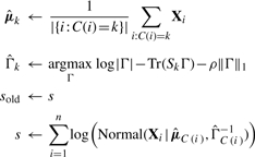
3. Re-assign: re-assign data points to clusters using a temporary cluster assignment function C_tmp (assignment becomes permanent if algorithm is not stopped in 4), and store smallest cluster size in m:

   
4. Iterate or terminate: stop if reach maximum number of iterations T, cluster size becomes too small or relative change in log-likelihood model score is below a threshold τ:

   

In all experiments below, we set T = 100, n_min = 4 and τ = 10⁻⁸. The penalty parameter ρ is set at the start of the procedure following Banerjee et al. (2008) [see also Meinshausen and Bühlmann (2006) for further details],

(2)

where is the sample variance for variable i and t_N−2(α), α ∈ [0, 1] is the quantile function of the Student's t-distribution with N − 2 degrees of freedom. Lower α gives sparser solutions (and a more biased estimate); we use a conservative choice of α = 0.1 in all experiments below. Optimization is carried out using the Banerjee/Nesterov procedure. The worst-case time complexity of our algorithm is 𝒪(TKp^4.5/ϵ) where ϵ > 0 is desired accuracy for the Nesterov optimization procedure (Banerjee et al., 2008).

This overall approach can be thought of as analogous to a standard iterative clustering, but with sparse graphical models used to define clusters. In all our experiments, we used the best result (i.e. the highest overall model score s) over 100 random initializations.

3 RESULTS

We show results on synthetic data, mixed data in which phospho-proteomic data were combined with synthetic data and on proteomic data obtained from cancer cell lines that are part of the NCI-60 panel. We are interested in examining the ability of ℓ₁-penalized network clustering to carry out two related tasks. First, to discover data subsets defined by network structure, i.e. to cluster with respect to underlying covariance structure. Second, to recover such subset-specific network structure. We assess the performance on both tasks below.

3.1 Synthetic data

Our simulation strategy was as follows. For each of two clusters, we generated data having known sparse inverse covariance structure. We then withheld cluster labels and analysed the data in an unsupervised manner to generate the results shown here. Sparse covariance structures were specified following a procedure described in Banerjee et al. (2008). A specified number of non-zero entries were randomly, symmetrically placed to create a precision matrix (corresponding to a graphical model with a specified number of edges) and then data were generated from the corresponding Gaussian model. The number of non-zero entries was set to equal the number of variables p. In the experiments below, we set p = 10 and used per-cluster sample sizes of n = 20, 30, 40, 50. To mimic the case in which biological subtypes differ subtly in terms of network structure, the cluster-specific network structures shared 6 out of 10 edges and each variable was set to have unit within-cluster variance. We are interested in the challenging case in which clusters differ at the network level, but are similar at the level of mean response, we therefore set the cluster means to differ by a small amount (0.75 in all experiments below).

3.1.1 Clustering

Figure 1 shows results for 100 simulated datasets, comparing ℓ₁-penalized network clustering with (i) K-means; (ii) a recently introduced, message-passing-based algorithm called affinity propagation (Frey and Dueck, 2007); (iii) diagonal-covariance Gaussian mixture model (GMM) using expectation–maximisation (EM); (iv) full-covariance GMM using EM; and (v) network clustering using an alternative network learning method due to Schäfer and Strimmer (2005) [this is rooted in shrinkage estimation; algorithm was as above with shrinkage estimation as described in Schäfer and Strimmer (2005) used in place of ℓ₁-penalized estimation]. We used the function kmeans within the MATLAB statistics toolbox (with K = 2 and 1000 random initialisations). Affinity propagation was used with default settings (pair-wise similarities equal to negative Euclidean distance and scalar self-similarity set to median similarity). EM was performed using the gmmb_em function within the MATLAB GMMBAYES toolbox (Paalanen et al., 2006) (with K = 2, 100 random initializations and maximum number of iterations set to T = 1000; other stopping criteria were the same as network clustering, namely n_min = 4 and τ = 10⁻⁸). All computations were carried out in MATLAB R2009a.

Fig. 1.

Simulated data, clustering results. Boxplots over the Rand index with respect to true cluster membership (higher scores indicate better agreement with the true clustering; a score of unity indicates perfect agreement) are shown for sample sizes of (a) n = 20, (b) n = 30, (c) n = 40 and (d) n = 50 per cluster. Data were generated for two clusters from known sparse network models (for details see text), with 100 iterations carried out at each sample size. Results shown for K-means (KM), affinity propagation (AP), diagonal-covariance Gaussian mixture model [GMM (diag)], full-covariance GMM [GMM (full)], network clustering using shrinkage-based network learning (NC:shrink) and ℓ₁-penalized network clustering (NC:L₁). (For n = 20 the full-covariance GMM could not be used as small-sample effects meant that it did not yield valid covariance matrices.)

We show boxplots over the Rand index with respect to the true cluster labels (the Rand index is a standard measure of similarity between clusterings; 1 indicates perfect agreement and 0 complete disagreement). The proposed ℓ₁-penalized network clustering shows consistent gains relative to the other approaches. At all but the smallest sample size, it is able to closely approximate the correct clustering, with high Rand indices, even when other methods do not perform well. The shrinkage-based network clustering approach also performs well, but is less effective than ℓ₁-penalization at all but the largest sample size. In contrast, K-means, affinity propagation and diagonal-covariance GMMs do not perform well, even in the largest sample case. This reflects the fact that these methods are not able to describe the cluster-level covariance structure that is crucial in this setting. A full-covariance GMM provides gains over the aforementioned three methods, but is both less effective and more variable than network clustering. This is due to the fact that conventional full covariance estimators can be ill-behaved at small sample sizes (indeed, in the n = 20 case a conventional full-covariance GMM did not yield valid covariance matrices and therefore could not be employed).

3.1.2 Network reconstruction

Figure 2 compares true, cluster-specific sparsity patterns (i.e. network structures) with those inferred by network clustering. We show results for network clustering (both ℓ₁-penalized and shrinkage-based) and from a GMM. Following the suggestion of a referee, we also show results obtained from the application of ℓ₁-penalized network learning to data from the clusters obtained by a GMM and K-means. We are motivated by settings in which underlying biological heterogeneity at the network level has remained unrecognized. Then, the default approach is to carry out network inference on the entire, heterogeneous dataset, without clustering. Results are shown also for this case; to allow a fair comparison, we use the same ℓ₁-penalized network inference method as is used for network clustering.

Fig. 2.

Simulated data, network reconstruction. Distance between true and inferred networks, in terms of the number of edge differences or ‘Structural Hamming Distance (SHD; smaller values indicate closer approximation to true network) for simulated data at sample sizes of n = 20, 30, 40, 50 per cluster. Results shown for: ℓ₁-penalized network inference applied to complete data, without clustering (‘All Data & L₁’); K-means clustering followed by ℓ₁-penalized network inference applied to the clusters discovered (‘KM & L₁’); clustering using a (full covariance) Gaussian mixture model followed by ℓ₁-penalized network inference [‘GMM (full) & L₁’]; full covariance GMM [‘GMM (full)’]; network clustering using ℓ₁-penalized network inference (‘NC:L₁’); and network clustering using shrinkage-based network inference (‘NC:shrink’). Mean SHD over 100 iterations are shown, and error bars indicate SEM.

We quantified the ability of network clustering to recover cluster-level structure by computing the SHD between true and estimated cluster-specific graphs. The SHD is equal to the number of edges that must be changed (added or deleted) to recover the true graph; lower scores indicate a closer match to the true structure. Figure 2 shows SHD, as a function of sample size, for the various approaches described above. At all sample sizes, network clustering provides reductions in SHD relative to the other approaches. Shrinkage network clustering performs well in this regard at larger sample sizes, while ℓ₁ network clustering does better at the smallest sample size. In contrast, inference without clustering is unable to recover network structure, and displays no improvements with sample size, despite the use of state-of-the-art sparse ℓ₁-penalized network inference. The GMM is outperformed by network clustering methods at all sample sizes, yet provides gains over network inference without clustering at all but the smallest sample size. (In all cases, we generated graphs from inverse covariance matrices by thresholding to induce p edges; our main conclusions were robust to the precise threshold used.)

3.2 Phospho-proteomic and synthetic data

We applied network clustering to a proteomic dataset from Sachs et al. (2005) pertaining to cell signalling. We used the Sachs et al. dataset to generate network heterogeneity in the following way. First, we subsampled n = 40 data points (without replacement) from the complete data (baseline data only, total of 853 samples, p = 11 phospho-proteins). Then, we merged these subsampled data with data generated using a known network structure (as described above; as above within-cluster marginal variances were unity). This gave a single, heterogeneous dataset with a total sample size of N = 80. To challenge the analysis and reflect the case in which biological subtypes differ with respect to underlying signalling networks but not in terms of mean phospho-protein abundance, we set the cluster means to differ by a small amount relative to the unit marginal variance (0.75, as above).

3.2.1 Clustering

Figure 3 shows clustering results obtained from the Sachs et al. phospho-proteomic data. As before, we compare ℓ₁-penalized network clustering with K-means, affinity propagation, diagonal-covariance and full-covariance GMMs and shrinkage-based network clustering (settings as described above). We show boxplots over the Rand index with respect to the true cluster labels over 100 datasets generated by subsampling as described above.

Fig. 3.

Phospho-proteomic and synthetic data, clustering results. Boxplots over the Rand index with respect to true cluster membership (score of unity indicates perfect agreement with the true clustering). Data with a known, gold-standard cluster assignment were created using phospho-proteomic data from Sachs et al. (2005) as described in text. Boxplots are over 100 subsampling iterations; per-cluster sample size was n = 40; algorithms used were K-means (KM), affinity propagation (AP), diagonal-covariance Gaussian mixture model [GMM (diag)], full-covariance GMM [GMM (full)], network clustering using shrinkage-based network inference (NC:shrink) and ℓ₁-penalized network clustering (NC:L₁).

3.2.2 Network reconstruction

Figure 4a shows SHD (computed as described above) between estimated and correct graphs¹ (these were induced from corresponding inverse covariance matrices by thresholding to return p edges; the result did not depend on precise threshold) over 100 iterations of subsampling. Network clustering provides reductions in SHD (i.e. more accurate network reconstruction) relative to the other methods used. Figure 4b–d compares the correct inverse covariance for the proteomic data² to estimates of it. Network clustering is able to recover the overall inverse covariance pattern or network structure. In contrast, applying ℓ₁-penalized network learning directly to the small-sample, heterogeneous data, without clustering, we find that the correct structure is obscured.

Fig. 4.

Phospho-proteomic and synthetic data, network reconstruction. (a) SHD between correct and inferred networks. Results shown for ℓ₁-penalized network inference applied to complete data, without clustering (‘All Data & L₁’); K-means clustering followed by ℓ₁-penalized network inference applied to the clusters discovered (‘KM & L₁’); clustering using a (full covariance) Gaussian mixture model followed by ℓ₁-penalized network inference [GMM (full) & L₁’]; clustering and network inference using a GMM [‘GMM (full)’]; network clustering using ℓ₁-penalized network inference (‘NC:L₁’); and network clustering using shrinkage-based network inference (‘NC:shrink’). Mean SHD over 100 subsampling iterations were shown, and error bars indicate SDs; (b) Correct sparsity pattern. Correct, large-sample sparsity pattern for proteomic data of Sachs et al. (2005); (c) NC:l₁. Inverse covariance recovered from small-sample, heterogenous data by ℓ₁-penalized network clustering and (d) All data (no clustering)-l₁. Inverse covariance from ℓ₁-penalized network inference applied directly to the complete, heterogenous data (see text for full details; per-cluster sample size n = 40; red and blue indicate negative and positive values, respectively).

3.3 Cancer proteomic data

We applied our network clustering method to proteomic data obtained from cell lines belonging to the National Cancer Institute's NCI-60 panel (Shankavaram et al., 2007). Specifically, we used proteomic data from the 10 melanoma cell lines and 8 renal cell lines within the panel. This gave a combined dataset with two subsets corresponding to cancer type, and a total of N = 18 samples. We used data for p = 147 proteins which did not show strong differential expression between the cancer types (raw P-values under a Welch two-sample t-test all exceed 0.001; total number of proteins in original dataset was 162; in addition to the P-value threshold, 7 proteins with erroneous zero values were discarded). These proteins cover a broad range of signalling pathways (see Supplementary Table S1). These data represent a high-dimensional setting in which cancer type labels are known (but withheld from the algorithms), thereby allowing objective assessment of clustering accuracy with respect to the labels.

Table 1 shows clustering results obtained from these data. Methods and settings are as described above. Despite the high dimensionality and low sample size of the data, ℓ₁-penalized network clustering is able to make a good approximation to the subtype labels. Indeed, over 100 iterations, the single highest model score s gave the correct clustering. Supplementary Figures S1 and S2 show the estimated inverse covariances for the two cancer types. We note that while ℓ₁-penalized network clustering provides gains relative to the other methods, the shrinkage-based approach does not. This is likely due to the small sample size, and echoes simulation results above. We note that a conventional full-covariance GMM approach was not applicable here as, due to the high dimensionality with respect to sample size, it does not yield valid (symmetric and positive definite) covariance matrices.

Table 1.

Clustering results for proteomic data from cancer cell lines

KM	AP	GMM (diag)	NC:sh	NC:ℓ1
0.58 ± 0	0.69*	0.62 ± 0.11	0.55 ± 0.08	0.80 ± 0.14

Mean Rand indices ±SD for K-means (KM), affinity propagation (AP), diagonal-covariance Gaussian mixture model [GMM (diag)], shrinkage-based network clustering (NC:shrink) and ℓ₁-penalized network clustering (NC:ℓ₁); results shown over 100 iterations, each with 100 random initializations (*except for AP which is a deterministic algorithm). Small sample proteomic data, obtained from melanoma and renal cell lines from the NCI60 panel, were clustered as described in Main Text (p = 147 proteins, full list in Supplementary Table S1; total sample size N = 18). Rand indices were calculated with respect to labels indicating the known cancer type (melanoma or renal) of each sample.

4 DISCUSSION AND FUTURE WORK

In this article, we addressed the question of probing molecular heterogeneity in settings where (hitherto uncharacterized) biological subtypes differ with respect to network structure. We did so by introducing a network clustering approach which takes advantage of the recent developments in efficient, ℓ₁-penalized learning of undirected graphical models. The approach proposed permits both the discovery of biological subtypes which differ at the network level and inference about underlying network structures.

The ideas presented here are closely related to a number of classical multivariate methods. We can think of network clustering as an unsupervised quadratic discriminant analysis with cluster-conditional models having sparse inverse covariances. Unfavourable conditions of dimensionality and sample size are exacerbated in clustering-type analyses because the limiting factor becomes not just the overall sample size (which may already be small), but rather the size of the smallest cluster (or, from a mixture model point of view, the smallest mixing coefficient). For this reason, some form of sparsity, regularization or shrinkage is crucial if full-covariance models are to be used for network clustering. From this point of view, the approach taken here, of emphasizing sparsity by the use of ℓ₁-penalization, is just one of several possible choices, but in the biological setting, where sparsity is arguably a reasonable assumption, an attractive one. An alternative approach to the ‘hard’ assignments used here would be a EM algorithm; this would yield in effect a mixture model formulation with sparse covariance structure. We also note that since the approach presented here builds on a well-understood, probability model-based clustering framework, many existing diagnostic procedures (e.g. for statistical significance, determining number of clusters, etc.) are readily applicable.

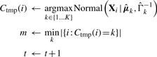
The network clustering problem is challenging, but one that we believe will become increasingly important as emphasis shifts from individual genes/proteins to networks, motivating covariance- rather than mean-centred formulations. In this article, we sought to formulate and address this problem in a tractable way and therefore focused on the simplest case of two clusters. However, the approaches introduced here apply also to the general K-cluster case. Figure 5 shows network clustering applied to simulated data from K = 3, 4 clusters [simulation regime as above, with all clusters sharing 6 out of 10 edges and cluster-specific means differing by a small amount (0.75, as above) from a zero mean cluster].

Fig. 5.

Simulated data, clustering results for K = 3, 4 clusters. Boxplots over the Rand index with respect to true cluster membership are shown for data consisting of (a) K = 3 clusters and (b) K = 4 clusters, with per cluster sample size of n = 50. Data were generated from known sparse network models (for details see text), with 25 iterations carried out at each sample size. Results shown for K-means (KM), affinity propagation (AP), diagonal-covariance Gaussian mixture model [GMM (diag)], full-covariance GMM [GMM (full)], network clustering using shrinkage-based network inference (NC:shrink) and ℓ₁-penalized network clustering (NC:L₁).

We based our approach on continuous, undirected graphical models, exploiting recent results in computationally efficient, optimization-based learning for these models. Directed graphical models, including Bayesian networks (BNs) and their variants, have been popular in the study of biological networks (including Husmeier, 2003; Mukherjee and Speed, 2008; Sachs et al., 2005; Segal et al., 2003; Yu et al., 2004). However, structural inference for BNs remains challenging and for networks of even moderate size, is typically computationally intensive. Since in the network clustering setting, efficient inference is essential to render the overall analysis tractable, we chose to eschew BNs here. (For example, for the cancer proteomic data, a single round of ℓ₁-penalized network inference for p = 147 variables required 7 s on a standard desktop computer; BN-based network inference for p = 147 variables would require minutes to many hours depending on the precise approach employed.) However, BNs are in many ways well suited to the study of gene regulatory and cell signalling networks and have been well developed for these applications in recent years. For this reason, we think that a promising line of research will be in developing BN-based network clustering approaches which extend the work presented here towards directed models.

REFERENCES

- Banerjee O., et al. Model selection through sparse maximum likelihood estimation for multivariate Gaussian or binary data. J. Mach. Learn. Res. 2008;9:485–516. [Google Scholar]
- Chuang H.Y., et al. Network-based classification of breast cancer metastasis. Mol. Syst. Biol. 2007;3 doi: 10.1038/msb4100180. Article 140. [DOI] [PMC free article] [PubMed] [Google Scholar]
- Dempster A.P. Covariance selection. Biometrics. 1972;28:157–175. [Google Scholar]
- Dobra A., et al. Sparse graphical models for exploring gene expression data. J. Multivar. Anal. 2004;90:196–212. [Google Scholar]
- Frey B.J., Dueck D. Clustering by passing messages between data points. Science. 2007;315:972–976. doi: 10.1126/science.1136800. [DOI] [PubMed] [Google Scholar]
- Friedman N. Inferring cellular networks using probabilistic graphical models. Science. 2004;303:799–805. doi: 10.1126/science.1094068. [DOI] [PubMed] [Google Scholar]
- Friedman J., et al. Sparse inverse covariance estimation with the graphical lasso. Biostatistics. 2008;9:432–441. doi: 10.1093/biostatistics/kxm045. [DOI] [PMC free article] [PubMed] [Google Scholar]
- Husmeier D. Reverse engineering of genetic networks with Bayesian networks. Biochem. Soc. Trans. 2003;31:1516–1518. doi: 10.1042/bst0311516. [DOI] [PubMed] [Google Scholar]
- Jones B., et al. Experiments in stochastic computation for high-dimensional graphical models. Stat. Sci. 2005;20:388–400. [Google Scholar]
- Jordan M.I. Graphical models. Stat. Sci. 2004;19:140–155. [Google Scholar]
- Koller D., Friedman N. Probabilistic Graphical Models: Principles and Techniques. Cambridge, MA: The MIT Press; 2009. [Google Scholar]
- Lauritzen S.L. Graphical Models. New York: Oxford University Press; 1996. [Google Scholar]
- Meinshausen N., Bühlmann P. High-dimensional graphs and variable selection with the Lasso. Ann. Stat. 2006;34:1436–1462. [Google Scholar]
- Mukherjee S., Speed T.P. Network inference using informative priors. Proc. Natl Acad. Sci. USA. 2008;105:14313–14318. doi: 10.1073/pnas.0802272105. [DOI] [PMC free article] [PubMed] [Google Scholar]
- Nesterov Y. Smooth minimization of non-smooth functions. Math. Prog. 2005;103:127–152. [Google Scholar]
- Paalanen P., et al. Feature representation and discrimination based on Gaussian mixture model probability densities–practices and algorithms. Pattern Recogn. 2006;39:1346–1358. [Google Scholar]
- Perou C., et al. Molecular portraits of human breast tumours. Nature. 2000;406:747–752. doi: 10.1038/35021093. [DOI] [PubMed] [Google Scholar]
- Ravikumar P., et al. High-dimensional Ising model selection using ℓ1-regularized logistic regression. Ann. Stat. 2010;38:1287–1319. [Google Scholar]
- Rue H., Held L. Gaussian Markov Random Fields: Theory and Applications. Boca Raton, FL, USA: Chapman & Hall/CRC; 2005. [Google Scholar]
- Sachs K., et al. Causal protein-signaling networks derived from multiparameter single-cell data. Science. 2005;308:523–529. doi: 10.1126/science.1105809. [DOI] [PubMed] [Google Scholar]
- Schäfer J., Strimmer K. A shrinkage approach to large-scale covariance matrix estimation and implications for functional genomics. Stat. Appl. Genet. Mol. Biol. 2005;4 doi: 10.2202/1544-6115.1175. Article 32. [DOI] [PubMed] [Google Scholar]
- Segal E., et al. Module networks: identifying regulatory modules and their condition-specific regulators from gene expression data. Nat. Genet. 2003;34:166–176. doi: 10.1038/ng1165. [DOI] [PubMed] [Google Scholar]
- Shankavaram U., et al. Transcript and protein expression profiles of the NCI-60 cancer cell panel: an integromic microarray study. Mol. Cancer Ther. 2007;6:820–832. doi: 10.1158/1535-7163.MCT-06-0650. [DOI] [PubMed] [Google Scholar]
- Sørlie T., et al. Gene expression patterns of breast carcinomas distinguish tumor subclasses with clinical implications. Proc. Natl Acad. Sci. USA. 2001;98:10869–10874. doi: 10.1073/pnas.191367098. [DOI] [PMC free article] [PubMed] [Google Scholar]
- Speed T.P., Kiiveri H.T. Gaussian Markov distributions over finite graphs. Ann. Stat. 1986;14:138–150. [Google Scholar]
- Tan C., et al. Comparative analysis reveals conserved protein phosphorylation networks implicated in multiple diseases. Sci. Signal. 2009;2:ra39. doi: 10.1126/scisignal.2000316. [DOI] [PubMed] [Google Scholar]
- Tibshirani R. Regression shrinkage and selection via the lasso. J. Roy. Stat. Soc. Ser. B. 1996;58:267–288. [Google Scholar]
- Yip K., Gerstein M. Training set expansion: an approach to improving the reconstruction of biological networks from limited and uneven reliable interactions. Bioinformatics. 2009;25:243–250. doi: 10.1093/bioinformatics/btn602. [DOI] [PMC free article] [PubMed] [Google Scholar]
- Yu J., et al. Advances to Bayesian network inference for generating causal networks from observational biological data. Bioinformatics. 2004;20:3594–3603. doi: 10.1093/bioinformatics/bth448. [DOI] [PubMed] [Google Scholar]
- Zhu X., et al. Getting connected: analysis and principles of biological networks. Genes Dev. 2007;21:1010–1024. doi: 10.1101/gad.1528707. [DOI] [PubMed] [Google Scholar]
Associated Data
This section collects any data citations, data availability statements, or supplementary materials included in this article.