Multiplexed shotgun genotyping for rapid and efficient genetic mapping

Abstract

We present a new approach to genotyping based on multiplexed shotgun sequencing that can identify recombination breakpoints in a large number of individuals simultaneously at a resolution sufficient for most mapping purposes, such as quantitative trait locus (QTL) mapping and mapping of induced mutations. We first describe a simple library construction protocol that uses just 10 ng of genomic DNA per individual and makes the approach accessible to any laboratory with standard molecular biology equipment. Sequencing this library results in a large number of sequence reads widely distributed across the genomes of multiplexed bar-coded individuals. We develop a Hidden Markov Model to estimate ancestry at all genomic locations in all individuals using these data. We demonstrate the utility of the approach by mapping a dominant marker allele in D. simulans to within 105 kb of its true position using 96 F1-backcross individuals genotyped in a single lane on an Illumina Genome Analyzer. We further demonstrate the utility of our method by genetically mapping more than 400 previously unassembled D. simulans contigs to linkage groups and by evaluating the quality of targeted introgression lines. At this level of multiplexing and divergence between strains, our method allows estimation of recombination breakpoints to a median of 38-kb intervals. Our analysis suggests that higher levels of multiplexing and/or use of strains with lower levels of divergence are practicable.

Reductions in the cost of high-throughput sequencing have allowed rapid advances in genotyping that promise unparalleled resolution in studies of the genetic architecture of complex traits (Ding and Jin 2009; Edenberg and Liu 2009; Ragoussis 2009). For example, SNP-based methods (e.g., RT–PCR, Sequenom MassARRAY, Illumina GoldenGate) can provide efficient genotyping of a relatively small number of markers in a large number of individuals. In contrast, array-based genotyping methods (e.g., Affymetrix, Agilent, etc.) can provide genotypes for a much larger number of markers (e.g., Coop et al. 2008; Mancera et al. 2008), though genotyping a large number of samples can be prohibitively expensive for many investigators. In fact, an awkward gap in methods persists for studies that require cost-effective typing of hundreds to thousands of markers in hundreds to thousands of individuals. Multiplexed genotyping at this intermediate scale would facilitate the construction of genetic maps, the mapping of induced mutations, and the mapping of quantitative trait loci (QTLs) both in model organisms and in non-model systems. This “genotyping gap” has led to the recent refinement of methods for bulk-segregant analysis (Lai et al. 2007; Baird et al. 2008; Ehrenreich et al. 2010; Wenger et al. 2010) that can provide accurate information on QTL location, but at the expense of individual-genotype information that may be desired, for example, to estimate allele effect sizes and epistasis.

Many genotyping methods involve a two-step process: First, informative SNPs are identified and, second, genotypes for these SNPs are scored in multiple individuals using any of a variety of technologies. Two recently published approaches used next-generation sequencing to combine marker discovery and genotyping in a single step (Baird et al. 2008; Huang et al. 2009). Both methods can generate a large number of genome-wide markers and can accommodate multiplexing of individuals. However, the restriction-site associated DNA (RAD) approach of Baird et al. (2008) is labor intensive, involving restriction enzyme digestion, mechanical shearing of DNA and repair, two independent ligations of adaptors, and two gel-purification steps. The “whole-genome resequencing” (WGR) approach of Huang et al.(2009) is simpler than RAD, but still involves DNA shearing and repair prior to adaptor ligation. Shearing and repair, a key feature of RAD, WGR, and other approaches based on the standard Illumina-library preparation protocols is expensive, labor intensive, and typically requires a large quantity of starting genomic DNA (i.e., up to 1 μg) (Baird et al. 2008). This requirement makes such approaches difficult to apply to nonclonal species that have small body sizes, such as Drosophila and other insects.

Here we propose an approach that we call “multiplexed shotgun genotyping” (MSG), which is similar in spirit to RAD and WGR, but combines the best aspects of both. Like RAD, our method is based on restriction enzyme (RE) digestion of genomic DNA. However, while RAD generally uses a rare-cutter RE, followed by shearing into smaller fragments, we use a more frequent cutter that allows us to ligate adapters to a large number of small genomic fragments in a single step and reduce the number of gel-purification steps from two to just one. In addition, the orientation of fragments is random with respect to the direction of sequencing, increasing their potential for revealing informative sequence differences. Since our method does not require shearing and repair of DNA prior to adapter ligation, this highly simplifies the library preparation protocol and allows us to start with very small amounts of genomic DNA from each individual (i.e., 10 ng).

Sequencing this library results in a large number of sequences widely distributed across the genome. We also developed a statistical framework to assign ancestry to chromosomal segments and detect recombination breakpoints based on a Hidden Markov Model. As an alternative to making hard assignments of chromosomal segments to one parent or the other (e.g., Xie et al. 2010), we use “soft” ancestry assignments in the form of a probability distribution on the ancestry, as proposed and implemented in a variety of similar contexts (e.g., Falush et al. 2003). This approach is highly suited to data in which the coverage, and thus the precision with which breakpoints can be localized, varies among individuals in a multiplexed genotyping experiment. We demonstrate efficient multiplexing of 96 individuals in a single library and our results indicate that even higher levels of multiplexing are practical.

Results

Multiplexed shotgun sequencing (MSG)

We developed a simple method to generate a large number of sequence reads widely scattered across the genome and to assign ancestry to chromosomal segments based on this information. Our approach starts from the premise that the strains under study display shared synteny across the genome with an existing genome sequence, and that the sequences of the study strains and the existing genome are sufficiently similar so that most short reads can be mapped to the genome with high accuracy. The availability of reference genome sequences obviates the need to pre-ascertain SNPs or to score a particular set of SNPs with a high degree of certainty. This is because a genome sequence provides abundant physical linkage information that can be exploited to impute ancestry at most locations in the genome. Thus, there is no requirement to score all individuals at the same loci. Instead, each individual can be scored at a different constellation of loci, and ancestry at all loci for all individuals can be imputed based on known physical linkage relationships.

To evaluate the efficiency and accuracy of our approach, we prepared a multiplexed shotgun library of 96 progeny (48 males and 48 females) from an F1-backcross experiment. Specifically, D. simulans w⁵⁰¹ was crossed to D. sechellia w¹. These closely related species can be crossed to generate fertile F1 females and sterile F1 males (Lachaise et al. 1986). The F1 females were subsequently backcrossed to males of the D. sechellia w¹ parental strain. The genomes of the two parental species are ∼2% divergent at the nucleotide level (Kliman et al. 2000). A total of 10 ng of genomic DNA from each individual was digested with the restriction enzyme MseI and 96 custom-designed adapters, each carrying a unique 6-bp barcode, were ligated to the restriction fragments (Fig. 1). The ligation reactions were combined, fragments were size-selected, and standard Illumina flow-cell adaptors were added using PCR with custom-designed primers. Sequencing this library produced ∼22 million 101-bp reads in a single lane of an Illumina Genome Analyzer.

Figure 1.

The experimental and bioinformatic pipeline for MSG. (1) Genomic DNA is fragmented with a restriction enzyme (RE) that leaves “sticky ends.” (2) Individual bar-coded adaptors are ligated to these restriction fragments. (3) Samples are pooled and, (4) the ligation products are size selected, PCR-amplified, and (5) sequenced on an Illumina Genome Analyzer. (6) Reads from the sequencing run are parsed based by barcode. (7) Each read is mapped to each of two parental genomes (indicated as red and blue, respectively). (8) Ancestry of chromosomal segments (blue: homozygous for parent 1; red: homozygous for parent 2; no color: heterozygous) is estimated using a Hidden Markov Model (HMM). (9) Genotypes and recombination breakpoints are used in downstream analyses, such as QTL mapping.

Sequences were parsed into 96 groups—representing the 96 backcross progeny—based on the barcode present at the beginning of each read. Using the Burrows-Wheeler Alignment tool (Li and Durbin 2009) with default settings, 52% and 69% of the reads mapped uniquely (i.e., to one genomic location with high confidence) to the D. simulans and D. sechellia parental reference genomes, respectively, and 29% of the reads mapped uniquely with no suboptimal matches to both genomes. For each sequence read, we considered only the first nucleotide difference distinguishing parental strains as “informative.” Supplemental Figure S1 shows the distribution of reads and informative markers among individuals. The median number of informative markers per individual was 15,070, corresponding to a marker density of ∼1 per 7 kb.

We developed a Hidden Markov Model (HMM) to assign ancestry to chromosomal segments in experiments that produce a large number of informative sequence reads across the genome of each individual (see Methods). An example of an HMM ancestry fit for a representative individual is shown in Figure 2. Blue and red vertical ticks along the top and bottom of each panel in Figure 2 represent individual informative SNP markers matching one parent or the other. We use the HMM to compute a posterior probability that a genomic region is either homozygous for parent one, homozygous for parent two, or heterozygous (Fig. 2). Supplemental Figure S1.3 shows the ancestry plot for the individual with the fewest informative reads out of the 96 multiplexed individuals. Since sequence reads for any particular individual are sparsely distributed across the genome, few individuals are typed at many of the same loci. We therefore used the HMM results to impute ancestry for all individuals at all genomic locations that were typed in at least one individual. Applying this procedure, we assigned ancestry at 125,214 genomic locations, effectively increasing our marker density to ∼1/kilobase.

Figure 2.

Genome-wide ancestry assignment for a representative individual. (A) The ancestry states are shown for all major chromosome arms for a representative (male) individual progeny from a (D. sechellia/D. simulans) F1 X D. sechellia backcross experiment. The posterior probability that a region is homozygous for D. simulans (red) or for D. sechellia (blue) ancestry is plotted along the y axis. A high probability of heterozygous ancestry is indicated as a solid black line across the center of the plot. (B–D) Closer examination of three breakpoints illustrates typical variation in breakpoint resolution. Gold shading represents the 95% confidence bounds on the position of crossovers and the coordinates for each of these bounds are shown at the bottom.

Localizing recombination breakpoints

Switches in the estimated ancestry state within a chromosome represent regions containing a recombination breakpoint (Fig. 2). We estimated the precision of recombination breakpoint estimation by calculating the genomic interval (in kilobases) over which the posterior probability in favor of a given ancestry state switched from >95% to <5%. Figure 3A plots the distribution of the 373 inferred breakpoint intervals in our experiment and shows that 50% of breakpoints can be localized to within 38 kb. The four breakpoints in Figure 3A that resolved to >200 kb belong to the least-covered individual (Supplemental Fig. S1). This individual had an informative marker density of ∼1/220 kb, which is threefold lower than the next-best covered individual. In addition to the density of informative markers, the resolution with which recombination breakpoints can be defined also depends on the sequencing error rate, ɛ, and uncertainty in the parental genomes, γ, which together determine the genotyping error rate (see Methods). Based on a separate experiment, in which we mapped parental reads generated with the same library preparation protocol to the parental genomes, we estimated the overall genotyping error rate to be ∼1%. The contribution of sequencing error (ɛ) to this is estimated from individual base qualities (see Methods). The remaining genotyping error is difficult to estimate; however, we found that varying γ between 0.5% and 2% in the HMM had little effect on the precision with which breakpoints could be resolved (Supplemental Material S2).

Figure 3.

Resolution of recombination breakpoints. (A) A histogram of 373 inferred recombination breakpoint intervals (coordinates where posterior probability of a given ancestry switches from ≥95% to ≤5%) for our backcross experiment. The red asterisks indicate the median breakpoint resolution in our experiment (96-plex, 2% divergence). (B,C) Box and whisker plots of the medians of 100 subsamples of the data to examine effects of (B) increased multiplexing and (C) decreased divergence between the strains being crossed.

The resolution with which breakpoints can be mapped also depends on the level of multiplexing in the experiment and on the level of divergence between the parental strains. We estimated the effects of multiplexing and divergence between the strains by subsampling our data. Figure 3B shows that increasing the number of individuals genotyped in a single sequencing lane from 96 to 384 would allow 50% of breakpoints to be resolved to ≤92 kb. Figure 3C shows that, at 96-plex, decreasing the level of divergence between parental strains from 2% to 0.5% would allow 50% of breakpoints to be resolved to ≤136 kb.

Utility in mapping a dominant phenotypic marker

To determine the utility of MSG for mapping studies, we previously engineered the D. simulans strain used in our F1-backcross experiment to carry a piggyBac transgene that drives Enhanced Yellow Fluorescent Protein (EYFP) from a Pax6 promoter, resulting in the dominant phenotype of fluorescent eyes. This transgene is located at position 7,139,931 bp on the D. simulans X chromosome (DL Stern, unpubl.). Of the 96 backcross progeny genotyped, 53 expressed EYFP in the eyes and 43 did not. QTL analysis using our method of genotyping and ancestry assignment revealed a single significant QTL peak on the X chromosome with a maximum LOD score at position 7,131,433 and a one-LOD support interval of 7,110,246–7,151,130 (Fig. 4). The maximum LOD is just 8498 bp from the marker's true location and, based on a more detailed analysis of inferred haplotypes (Fig. 4, inset), we could define a minimum interval of 104,069 bp containing the dominant marker.

Figure 4.

QTL map of the location of a dominant marker segregating in the reported backcross experiment. The inset illustrates below the estimated ancestries for all individuals between genomic locations 5.5 Mb and 8.5 Mb on the X chromosome and, above, the LOD profile. Individual ancestry estimates are sorted into individuals without EYFP above and with EYFP below. Regions with posterior probabilities close to 1 of homozygous D. simulans are coded blue, and homozygous D. sechellia are coded red. Posterior probabilities between 0 and 1 are coded with colors intermediate between blue and red.

Mapping unassembled contigs of the D. simulans genome assembly

One common result of genome projects is the assembly of many sequences into contigs that cannot be assembled into larger scaffolds or placed on chromosomes (Pop and Salzberg 2008). This is true even when genomes are “assembled” by alignment to a known genome sequence. For example, the D. simulans genome project involved placement of most contigs onto chromosomes by comparisons with the D. melanogaster genome (Clark et al. 2007). Nonetheless, the six assembled major chromosomal arm scaffolds of the D. simulans genome assembly comprise just 101 Mb of the ∼120-Mb euchromatic genome and 9999 unassembled contigs contain an additional ∼26 Mbp. Nine-hundred and two (∼10%) of these unassembled contigs of the D. simulans genome assembly are ≥5 kb, and together these comprise ∼50% of the DNA content of the unassembled genome. We reasoned that it should be possible to use our method to assign some of these larger unassembled contigs to genetic map locations.

Using our backcross data, we were able to assign ancestry to 1029 (∼10%) of the unassembled D. simulans contigs in at least six backcross progeny. We identified a unique mapping location in the genome with a maximum LOD score ≥2 for 404 of these unassembled contigs (Supplemental Material S3). Two hundred and ninety-six of these had already been assigned to one of six major chromosomal arms based on homology searches by the original genome project (Clark et al. 2007). We confirmed most of these assignments, but found reasonably strong evidence for incorrect assignment for 16 of these contigs. We are also able to assign 108 previously unassigned contigs to linkage groups. In total, we were able to assign 8 Mb (∼30%) of the unassembled genome to linkage groups using mapping data resulting from a single lane of Illumina Genome Analyzer.

Utility in evaluating introgression lines

Introgression mapping is a powerful method for identifying the genomic regions encoding phenotypic differences between strains or between species (Iakoubova et al. 2001). One widespread difficulty experienced in introgression experiments is ensuring that a genomic region has been introgressed cleanly from one strain into another without inadvertently introgressing other regions that may alter the phenotype under consideration. In addition, defining introgression breakpoints is time consuming and, therefore, breakpoint ends are rarely estimated with much precision. Our method provides a rapid and economical method for detecting and delimiting introgressed regions. For example, in Figure 5, we show the results of three experiments in which specific chromosome regions were targeted for introgression through selection of a dominant marker (indicated with a yellow arrow in Fig. 5). Targeted introgression of a dominant marker at position 9.4 Mb on 3R resulted in introgression of the surrounding region of 3R plus inadvertent introgression of a region of chromosome X in one case (Fig. 5A) and the telomere of chromosome 2L in another case (Fig. 5B). These small introgressions may have escaped detection if a more traditional panel of markers had been screened. Figure 5C demonstrates a clean introgression of a region on 2L through targeted introgression of a marker at position 5.9 Mb on 2L.

Figure 5.

Three representative individuals from an experiment involving targeted introgression of D. simulans genomic regions into a D. sechellia genomic background. The color scheme is the same as in Figure 2. Individuals in A and B carry an introgression of a genomic region on 3R that was targeted with a dominant marker located at 9,390,800 bp on chromosome 3R (DL Stern, unpubl.), but also carry regions with D. simulans ancestry on the X and the tip of 2L, respectively (arrows). (C) Introgression of a region on 2L that was targeted with a dominant marker located at 5,926,416 bp on chromosome 2L (DL Stern, unpubl.) with no residual regions of D. simulans ancestry.

Discussion

RAD (Baird et al. 2008), WGR (Huang et al. 2009), and the approach outlined here, MSG, help fill an awkward gap between current methods that allow efficient screening of many loci in a small number of samples and other methods that provide efficient screening of a small number of markers in a large number of individuals. Our approach provides three significant advantages over existing methods. First, it involves a highly simplified protocol for library preparation that requires ∼2 d of lab work to process 96 individuals or more. The technique is inexpensive because it requires only standard molecular laboratory equipment, uses only one set of bar-coded adapters, and does not require shearing and repair of genomic DNA nor the use of exotic enzymes or other reagents. Second, because our method does not depend on manual shearing, small amounts of DNA isolated from single individuals can be processed, which makes our approach ideal for application to small and nonclonal species, such as insects. Third, like Xie et al. (2010), our method implements an HMM algorithm to assign ancestry states to chromosomal segments. This has the advantage of providing a formal statistical framework for estimating ancestry, thus avoiding window-based approaches (e.g., Huang et al. 2009), and allows imputation of ancestry at genomic positions with missing data. An advantage of our HMM framework is that we work with the posterior probability distribution on ancestry states (“soft” rather than “hard” ancestry assignments). Thus, our method correctly propagates the uncertainties in individual ancestry assignments that necessarily arise around recombination breakpoints, a property that is particularly useful when dealing with highly multiplexed data where coverage is low and varies considerably among individuals. Our HMM can, of course, be applied to any other sources of genotyping data, including the results of RAD and WGR experiments.

We have applied our approach with a high degree of multiplexing that provided accurate and precise mapping of a dominant marker in the D. simulans genome by simultaneous genotyping of 96 backcrossed progeny. By subsampling from our experiment with 96 individuals, we found that higher levels of multiplexing, at least up to 384 individuals, are likely to provide sufficient resolution for most mapping studies. We have also demonstrated the utility of our approach in identifying misassembled regions of the genome and in assigning genetic map positions to misassembled and unassembled contigs. Mapping experiments like these are a potentially useful tool for verifying and improving de novo genome assemblies.

Since our method is based on restriction enzyme digestion, it cannot catalog all polymorphisms that distinguish two parental genomes. However, barring very dramatic improvements in sequencing throughput, the same limitation applies to multiplexed WGR, since coverage per individual is expected to be low in highly multiplexed samples. Like WGR, our approach will suffer when the level of divergence between the parental strains is low, because more coverage is needed per individual to recover a desired density of informative markers. Nonetheless, by subsampling our 96-plex data (101-bp reads), even divergence as low as 0.5% between parental strains allowed resolution of half of the recombination breakpoints to within 136 kb. This is sufficient resolution for QTL studies involving genotyping of hundreds of individuals (Mackay 2001). Clearly, there will always be a trade-off between marker density, read length, and the degree of multiplexing. Continued reductions in the cost of sequencing and increases in the length of sequence reads, and reducing the biased representation of reads across individuals, will provide further improvements in the performance of the method.

Drosophila species have small genomes relative to many eukaryotes; is our method applicable to much larger genomes? To address this question, we carried out an MSG experiment on simulated human–chimpanzee F1-backcross individuals, generated by creating 96 “recombinant F1-backcross individuals” using the human and chimpanzee reference genomes (Supplemental Material S4). These two species have ∼20-fold larger genomes than Drosophila but exhibit comparable levels of divergence (i.e., 1%) to the D. simulans and D. sechellia strains used in our backcross experiment. Using the same distribution of the number of reads per individual observed in our Drosophila cross data, we detected all 96 simulated recombination breakpoints, and all true breakpoints fell within the estimated breakpoint intervals. The resolution of these recombination breakpoints (Supplemental Fig. S4.1) is lower than observed in our Drosophila cross (the most appropriate comparison is Fig. 3C, 1% divergence). This is expected given that the same number of reads is being applied to a ∼20-fold larger genome, and we see a strong relationship between the number of reads and breakpoint resolution in our simulated data (Supplemental Fig. S4.3). We conclude that, given forthcoming advances in sequencing technology (e.g., Illumina's “HiSeq” technology, http://www.illumina.com/systems/hiseq_2000.ilmn), genome size per se is unlikely to limit the applicability of our approach.

Approaches like ours work best when crosses involve parental strains with genomes that have been fully sequenced and properly assembled. However, it should be noted that our approach requires a genome assembly for only one of the two parental species to establish the order of markers across the genome. In fact, preliminary data from our labs suggests that our approach works well with just one reasonably well-assembled genome, Drosophila yakuba (Clark et al. 2007), and a partial de novo assembly of a second genome, D. santomea (unpublished data). In principal, it should be possible to start with two partially assembled genomes and then infer marker order from genetic linkage data. To some extent we have already demonstrated this by genetically mapping unassembled contigs of the D. simulans genome. In recent years, many genome projects have been “completed”, with assemblies resulting in a large number of scaffolds and contigs. We suggest that, for at least some of these organisms, our approach could allow placement of many of these contigs along a genetic map. In addition, genetic linkage data for contigs produced by a first-pass assembly of short reads may facilitate de novo assembly of large eukaryotic genomes.

Our approach may be particularly useful in mapping mutations induced in genetic screens (Wang et al. 2010). In recent years, EMS-induced mutagenesis screens have become less common, in part because identifying the relevant mutation has, traditionally, been time-consuming (Chen et al. 1998; Martin et al. 2001). Our approach provides an extremely rapid and convenient means of mapping such mutations to small genomic intervals. Whole-genome sequencing alone may not result in direct identification of causal mutations, because most mutagenesis protocols result in production of multiple mutations per chromosome. However, combining whole-genome sequencing with a genetic mapping approach like MSG should allow rapid, direct identification of induced, causal mutations.

Methods

Fly lines and crosses

We generated recombinant hybrid progeny of D. simulans (strains: w⁵⁰¹ and w^Su1) and D. sechellia (strains: w¹ and 14021-0248.28) by backcrossing F1 females to males from either of the parental species (Supplemental Fig. S5). In one of these crosses (D. simulans w⁵⁰¹ X D. sechellia w¹), the D. simulans strain was constructed by injecting strain w⁵⁰¹ with a modified version of pBAC[3xP3-EYFP] (Horn and Wimmer 2000) and we mapped the position of the insertion to X: 7139931 of the D. simulans reference genome (DL Stern, unpubl.). Female F1 (D. simulans w⁵⁰¹ X D. sechellia w¹) were backcrossed to males of D. sechellia (D. sechellia w¹). We scored the presence or absence of this dominant phenotypic marker in eyes of adult flies and collected 53 EYFP+ and 43 EYFP− F1-backcross progeny flies for genotyping. Strain D. simulans w^Su1 carries an allele of white induced with EMS in strain 14021-0251.006, which was originally collected in Nueva, California (DL Stern, unpubl.). For analyses of targeted introgressions, we crossed one of two strains of D. simulans w^Su1 carrying EYFP markers at positions 3R:9390800 and on 2L:5926416, respectively, to D. sechellia 14021-0248.28 (DL Stern, unpubl.). Female progeny were backcrossed to male D. sechellia 14021-0248.28 for three generations and were selected each generation for the presence of the EYFP marker.

Bar-coded adapter design

The design of library linkers followed the standard Illumina adapter design for single read libraries (http://www.illumina.com) with several modifications. Three bases were removed from the 3′ end of the FC2 oligonucleotide and replaced with a 6-base bar code (ACACTCTTTCCCTACACGACGCTCTTCCGANNNNNN, where n = a barcode base). The barcode is designed to give 5 degrees of freedom (varying bases 2–6 allows 1024 distinct barcodes, see Supplemental Material S6). The first position of the barcode comprises a unique identifying base that makes all barcodes at least two steps away from the nearest barcode. In practice, we excluded barcodes with mononucleotide runs >2, leaving 962 barcodes (available on request). The phosphorylated FC1 oligonucleotide is designed to partially complement the above FC2 oligonucleotide, but also includes a 5′ TA (p-TAnnnnnnTCGGAAGAGCTCGTATGCCGTCTTCTGCTTG, where p = phosphate and nnnnnn = the reverse complement of the FC2 barcode). When annealed, the adapter has a 5′ TA overhang designed to complement the “sticky ends” produced by any restriction enzyme that leaves compatible ends. In this application, we used MseI, which recognizes the motif “TTAA” and is expected to cut about once every 125 bp in the Drosophila genome (assuming 40% GC content). Adapters were prepared by combining 1 nmol of each of a pair of oligonucleotides in 100 μL of reassociation buffer (10 mM Tris at pH 8, 50 mM NaCl, 1 mM EDTA), briefly heating the mixture to 95°C, and then allowing them to anneal overnight at room temperature, resulting in a 10-μM final concentration of annealed adapters.

Genomic DNA extraction

We modified the Puregene genomic DNA isolation kit for single Drosophila (Qiagen). Single flies were placed in individual wells of a 96-well round bottom polystyrene plate (Costar, #3788), with 100 μL of lysis buffer. We added a 5/32 inch stainless-steel ball (part# GBSS 156-5000-01, OPS Diagnostics) to each well, sealed the plate with PCR tape (Thermoscientific), and homogenized the flies for 7 min in a Talboys High Throughput homogenizer (Troemer). The plate was then spun at 800g for 8 min to precipitate fly cuticle. Eighty microliters of the homogenate from each well were transferred to a 0.2-mL 96-well PCR plate (Fisher, catalog # 14230237) and the solution was incubated at 65°C for 15 min. A total of 2 μg of RNaseA in a volume of 4 μL was added to each sample. The sealed plate was inverted 25 times and incubated at 37°C for 3 h. We then added 26.4 μL of the Puregene protein precipitation solution to each sample, and the plate was sealed with PCR tape. After mixing the sealed plate by gentle vortexing for 45 sec, the samples were centrifuged at 3200g for 35 min. Genomic DNA was precipitated by adding 80 μL of the resulting supernatant to 80 μL of isopropanol in a fresh 0.2-mL 96-well PCR plate. The sealed plate was mixed by inversion and incubated at −20°C for 15 min. The DNA was precipitated by centrifugation at 3200g for 35 min. We washed the DNA pellets with 80 μL of 70% EtOH, resuspended dried pellets in 20 μL of DNA hydration solution, and incubated at 65°C for 30 min. DNA was quantified using a Qubit flourimeter (Invitrogen). Alternatively, we quantified DNA in 96-well format using a Typhoon 9400 biomolecular imager (GE healthcare) with a modified version of a protocol described in the Amersham Biosciences Fluorescent Imaging Protocol Handbook (Amersham Biosciences).

Production of the bar-coded library

Using the calculated concentrations of DNA from the quantification step, we diluted genomic DNA to 1–10 ng/μL and transferred 10 ng of each sample to a clean 0.2-mL PCR plate. We digested genomic DNA in a volume of 20 μL with 3.3 U of MseI (New England Biolabs) for 3 h at 37°C, followed by heat inactivation at 65°C for 20 min. To attach bar-coded adapters, we added 5 nmol of unique bar-coded adapters into individual wells, along with a ligation solution containing 1 U of T4 DNA ligase (New England Biolabs) in a total volume of 50 μL. The sealed plate was mixed by gentle vortexing, spun briefly, and incubated at 16°C for 1 h. We next pooled the contents of each ligation reaction into a single tube, and the ligated products were concentrated by isopropanol precipitation (10% 3M NaOAc at pH 5.2, 1 μL glycogen, and 1 vol of 100% isopropanol). The library was resuspended in 100 μL of 1X Tris-EDTA (pH 8.0), extracted with Tris-EDTA (pH 8) saturated phenolchloroform, and once again with chloroform. We removed ligated linker-dimers using AMPure beads (Agencourt) at a bead-mixture:volume ratio of 1.5 and size-separated the library on a 2% GTG agarose gel (NuSieve). We then stained the gel with SYBR green (Invitrogen) and cut out a gel slice between 250 and 300 bp on a long-wavelength transilluminator. We extracted DNA from the gel slice using a Qiagen gel extraction kit and resuspended the library in 30 μL of elution buffer. To increasethe precision of the size selection, we added 2 μL of GeneRuler 50 bp DNA Ladder (Fermentas) directly to the resuspended library prior to electrophoresis to correct for the effects of salt and other factors on band migration in the gel.

Similar to the standard Illumina library protocol, we attached the FC2 flow cell sequence to ligation products with 15 cycles of PCR (Phusion high-fidelity, Finnzymes) using HPLC-purified primers (IDT) that are slight modifications of the standard Illumina primers: FC2_PCR, 5′-AATGATACGGCGACCACCGAGATCTACACTCTTTCCCTACACGACGCTCTTCCGA-3′; FC1_PCR, 5′-CAAGCAGAAGACGGCATACGAGCTCTTCCGA-3′. The 3′ end of these primers is modified with phosphorothioate, preventing degradation of the primer by error-correcting polymerases (Quail et al. 2008). The amplified library was flourometrically quantified on a Qubit flourimeter (Invitrogen) and sequenced on an Illumina Genome Analyzer (Princeton Microarray Facility, http://www.genomics.princeton.edu/microarray/) using the standard Illumina protocols. We used a sequencing primer that is a truncated version of the standard Illumina sequencing primer: 5′-ACACTCTTTCCCTACACGACGCTCTTCCGA-3′. A linker-dimer band was typically present following PCR and was removed using AMPure beads, as described above.

Parsing, mapping reads, and assigning ancestry

Our library sequencing protocol typically produced 10–20 million reads per lane of an Illumina Genome Analyzer flow cell. Sequences for backcrossed individuals from the F1-backcross experiment have been deposited in the Sequence Read Archive SRA025671; SRS118670. The sequences were first parsed by barcode and each read was assigned to an individual. Considerable variance in the number of reads per individual is observed (Supplemental Fig. S1, coefficient of variation: 0.89). We performed two additional experiments (Supplemental Fig. S7) that show that barcode identity and the starting quality of genomic DNA are both likely to contribute to this variation. This said, the coefficient of variation in the number of informative markers per individual (0.67) is considerably lower than the number of reads. While this variation does not pose a problem for the analyses outlined here, we are currently working on ways to mitigate this bias in order to improve the efficiency of the method under higher levels of multiplexing and lower levels of divergence between the crossed strains.

For all reads assigned to an individual, we used BWA (the Burrows-Wheeler Alignment tool) (Li and Durbin 2009) to map each read to both parental genomes, which produces two “sam” format (http://samtools.sourceforge.net) files for each individual. The resulting sam files were then filtered and only those reads that mapped uniquely (with no suboptimal matches) to both parental genomes were retained. Unlike traditional genotyping methods that rely on a well-established panel of SNPs, the use of whole genome shotgun sequencing of cross progeny is associated with uncertainty in the states of parental genomes. In addition, the processes of sequencing and mapping sequence reads to reference genomes—our analog to genotyping—are also subject to error. Since it would be advantageous to model these sources of error explicitly, we formulated a Hidden Markov Model (HMM) (Rabiner 1989) to estimate underlying genome-wide ancestry and the positions of recombination breakpoints (i.e., changes in ancestry of adjacent chromosome segments, see Supplemental Fig. S8). The emission probabilities in the model are parameterized by two error parameters (γ and ɛ) that serve to model uncertainty in parental genome sequence, as well as sequencing and mapping error. The assignment of ancestry to genomic segments has the advantage that it circumvents the need to type all markers in all individuals. In addition, as an alternative to making “hard” assignments to one parent or the other, our approach allows us to compute a posterior probability distribution on the ancestry of chromosomal segments. Such “soft” approaches have been previously applied in a variety of similar contexts (e.g., Falush et al. 2003) and are particularly well suited to our multiplexed sequence data, in which genome coverage varies considerably among individuals.

Let {AA, AB, BB} represent the three possible ancestry states at a locus in diploid progeny of a cross between parental strains A and B. Priors on these ancestry states depend on the crossing design and whether a chromosome is sex-linked (and potentially hemizygous in one sex). In the case of our F1 parent backcross experiment, if A represents D. simulans and B represents D. sechellia, then the priors are set to {0, 0.5, 0.5} for autosomes and the X chromosome in females and {0.5, 0, 0.5} for the X chromosome in males. The HMM for individual i features a sequence of latent variables Z_im ∈ {AA, AB, BB} representing the unknown ancestry state at locus m (see Supplemental Fig. S6). The transition probabilities (r_m,m+1) between states Z_im and Z_i(m+1) were set such that the average number of crossover events detected is on the order of one per chromosome (Ashburner 1989). The read data at locus m are contained in a count vector X_im, such that X_imj is the number of reads from individual i that mapped to locus m and that have allele j ∈ {A,C,G,T}. We modeled these counts as being multinomially distributed with cell probabilities depending on the genotype G_im of individual i at locus m, while allowing for errors. In general, the ancestry state Z_im contains information about G_im, but does not determine it unambiguously. Therefore, we computed the emission probabilities by averaging over the uncertainty in the genotype,

where Γ is a set containing the 10 possible diploid genotypes. We defined the two ancestry states by specifying “allele frequency distributions” at each locus, such that P_kmj is the probability of sampling allele j at locus m from ancestry background k ∈ {A,B}. The genotype probabilities in the mixture (Eqn. 1) are then given by

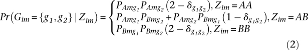in which δ_jj′ is an indicator variable that takes the value of 1 if j = j′ and the value of 0 otherwise. One can think of P as an expression of our confidence in the parental genome reference sequences to which reads were mapped. In the special case of homozygous inbred parental lines whose genome sequence may be considered known without error, ancestry uniquely determines genotype (the “allele frequency distributions” have probability 1 for one allele and 0 elsewhere) with the result that only one genotype contributes to the mixture (Eq. 1).

The values P can be defined at any level of detail, including specifying the individual parental genome reference (k) or specific positions within those sequences (m). In practice, we define P using just one parameter, γ, which reflects an average genome-wide uncertainty in both parental reference sequences. For example, if a given nucleotide state j exists at position m of parental reference genome k and is “C”, we define . We set γ_k = 0.01 for both parental genomes, and have found that our results are not affected much by varying γ by twofold (Supplemental Material S2).

Conditional on the diploid genotype, we model the read data as being generated by repeated sampling with replacement from these two alleles with sequence errors occurring with probability ɛ_im:

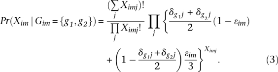We found that multiple reads mapping to individual sites in heterozygous regions were often invariant, suggesting that only one of the two parental alleles at this site is represented in the reads. This is not unexpected given the low level of coverage, on average, at particular loci. In practice, we therefore randomly sample one read at each marker locus. Future versions of the code will consider all reads at a locus, which will be appropriate for higher coverage data. The sequencing error, ɛ_im is estimated for each marker locus as 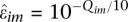, where Q _im corresponds to the Phred quality value of the base-call in the randomly sampled read.

We focused on the marginal posterior probability of ancestry at locus m, Pr(Z_im | X_i), which can be computed from equations 1–3 using standard algorithms for HMMs (Rabiner 1989). In the preceding description, the index m varies over those loci at which read data are available for individual i. After fitting the HMM for all individuals, we used linear interpolation to extend the model fit so that, in each individual, a posterior probability of ancestry is available at every position to which reads map in at least one individual. We measured the evidence for linkage between markers m and m′ with a version of the standard LOD statistic modified to use soft ancestry calls. The LOD statistic for markers m and m′ is a log likelihood ratio statistic testing the hypothesis that the recombination fraction r_mm′ is zero:

where n is the number of individuals. We compute this statistic using soft ancestry calls by using the posterior probability of ancestry at markers m and m′ to estimate the recombination fraction r_mm:

Software implementing the above analyses is available at http://genomics.princeton.edu/AndolfattoLab/MSG.html.

Parental genomes

Because we estimated ancestry using an HMM that incorporates uncertainty due to incomplete knowledge of the parental genomes (reflected in the parameter P), we did not require perfect knowledge of the parental genomes. In fact, our approach worked reasonably well when we used the reference genomes in lieu of the true parental genomes in the case of D. simulans and D. sechellia. Nonetheless, to reduce uncertainty in the parental genomes, we collected 20 million 95-bp reads from D. simulans w⁵⁰¹ (SRS139966.1), 21 million 95-bp reads from D. sechellia w¹(SRS139969.2), 6 million 70-bp reads from D. simulans w^su1, and 1 million 70-bp reads from D. sechellia strain 14021-0248.28. We prepared multiplexed libraries for these parental strains as described above, to maximize the degree of overlap among reads from parental strains and backcross progeny. These reads were mapped to the genome reference strains using BWA (as above) and the resulting pileup (SAMtools, http://samtools.sourceforge.net) was used to generate a consensus sequence for each of the parental strains. Applying our mapping approach to D. simulans and D. sechellia backcross progeny, we identified six regions of the D. simulans genome with anomalous segregation patterns (Supplemental Material S9). These regions were masked in subsequent analyses.

References

- Ashburner M 1989. Drosophila: A Laboratory Handbook. Cold Spring Harbor Laboratory Press, Cold Spring Harbor, NY [Google Scholar]
- Baird NA, Etter PD, Atwood TS, Currey MC, Shiver AL, Lewis ZA, Selker EU, Cresko WA, Johnson EA 2008. Rapid SNP discovery and genetic mapping using sequenced RAD markers. PLoS ONE 3: e3376 doi: 10.1371/journal.pone.0003376 [DOI] [PMC free article] [PubMed] [Google Scholar]
- Chen B, Chu T, Harms E, Gergen JP, Strickland S 1998. Mapping of Drosophila mutations using site-specific male recombination. Genetics 149: 157–163 [DOI] [PMC free article] [PubMed] [Google Scholar]
- Clark AG, Eisen MB, Smith DR, Bergman CM, Oliver B, Markow TA, Kaufman TC, Kellis M, Gelbart W, Iyer VN, et al. 2007. Evolution of genes and genomes on the Drosophila phylogeny. Nature 450: 203–218 [DOI] [PubMed] [Google Scholar]
- Coop G, Wen X, Ober C, Pritchard JK, Przeworski M 2008. High-resolution mapping of crossovers reveals extensive variation in fine-scale recombination patterns among humans. Science 319: 1395–1398 [DOI] [PubMed] [Google Scholar]
- Ding C, Jin S 2009. High-throughput methods for SNP genotyping. Methods Mol Biol 578: 245–254 [DOI] [PubMed] [Google Scholar]
- Edenberg HJ, Liu Y 2009. Laboratory methods for high-throughput genotyping. Cold Spring Harb Protoc 2009: doi. 10.1101/pdb.top62 [DOI] [PubMed] [Google Scholar]
- Ehrenreich IM, Torabi N, Jia Y, Kent J, Martis S, Shapiro JA, Gresham D, Caudy AA, Kruglyak L 2010. Dissection of genetically complex traits with extremely large pools of yeast segregants. Nature 464: 1039–1042 [DOI] [PMC free article] [PubMed] [Google Scholar]
- Falush D, Stephens M, Pritchard J 2003. Inference of population structure using multilocus genotype data: linked loci and correlated allele frequencies. Genetics 164: 1567–1587 [DOI] [PMC free article] [PubMed] [Google Scholar]
- Horn C, Wimmer EA 2000. A versatile vector set for animal transgenesis. Dev Genes Evol 210: 630–637 [DOI] [PubMed] [Google Scholar]
- Huang X, Feng Q, Qian Q, Zhao Q, Wang L, Wang A, Guan J, Fan D, Weng Q, et al. 2009. High-throughput genotyping by whole-genome resequencing. Genome Res 19: 1068–1076 [DOI] [PMC free article] [PubMed] [Google Scholar]
- Iakoubova OA, Olsson CL, Dains KM, Ross DA, Andalibi A, Lou K, Choi J, Kalcheva I, Cunanan M, Louie J, et al. 2001. Genome-tagged mice (GTM): Two sets of genome-wide congenic strains. Genomics 74: 89–104 [DOI] [PubMed] [Google Scholar]
- Kliman RM, Andolfatto P, Coyne JA, Depaulis F, Kreitman M, Berry AJ, McCarter J, Wakeley J, Hey J 2000. The population genetics of the origin and divergence of the Drosophila simulans complex species. Genetics 156: 1913–1931 [DOI] [PMC free article] [PubMed] [Google Scholar]
- Lachaise D, David R, Lemeunier F, Tsacas L 1986. The reproductive relationships of Drosophila sechellia with D. mauritiana, D. simulans, and D. melanogaster from the afrotropical region. Evolution 40: 262–271 [DOI] [PubMed] [Google Scholar]
- Lai CQ, Leips J, Zou W, Roberts JF, Wollenberg KR, Parnell LD, Zeng ZB, Ordovas JM, Mackay TF 2007. Speed-mapping quantitative trait loci using microarrays. Nat Methods 4: 839–841 [DOI] [PubMed] [Google Scholar]
- Li H, Durbin R 2009. Fast and accurate short read alignment with Burrows-Wheeler transform. Bioinformatics 25: 1754–1760 [DOI] [PMC free article] [PubMed] [Google Scholar]
- Mackay TFC 2001. Quantitative trait loci in Drosophila. Nat Rev Genet 2: 11–20 [DOI] [PubMed] [Google Scholar]
- Mancera E, Bourgon R, Brozzi A, Huber W, Steinmetz LM 2008. High-resolution mapping of meiotic crossovers and non-crossovers in yeast. Nature 454: 479–485 [DOI] [PMC free article] [PubMed] [Google Scholar]
- Martin SG, Dobi KC, St Johnston D 2001. A rapid method to map mutations in Drosophila. Genome Biol 2: RESEARCH0036 doi: 10.1186/gb-2001-2-9-research0036 [DOI] [PMC free article] [PubMed] [Google Scholar]
- Pop M, Salzberg SL 2008. Bioinformatics challenges of new sequencing technology. Trends Genet 24: 142–149 [DOI] [PMC free article] [PubMed] [Google Scholar]
- Quail MA, Kozarewa I, Smith F, Scally A, Stephens PJ, Durbin R, Swerdloro H, Turner DJ 2008. A large genome center's improvements to the Illumina sequencing system. Nat Methods 5: 1005–1010 [DOI] [PMC free article] [PubMed] [Google Scholar]
- Rabiner LR 1989. A tutorial on hidden Markov models and selected applications to speech recognition. Proc IEEE 77: 257–286 [Google Scholar]
- Ragoussis J 2009. Genotyping technologies for genetic research. Annu Rev Genomics Hum Genet 10: 117–133 [DOI] [PubMed] [Google Scholar]
- Wang H, Chattopadhyay A, Li Z, Daines B, Li Y, Gao C, Gibbs R, Zhang K, Chen R 2010. Rapid identification of heterozygous mutations in Drosophila melanogaster using genomic capture sequencing. Genome Res 20: 981–988 [DOI] [PMC free article] [PubMed] [Google Scholar]
- Wenger JW, Schwartz K, Sherlock G 2010. Bulk segregant analysis by high-throughput sequencing reveals a novel xylose utilization gene from Saccharomyces cerevisiae. PLoS Genet 6: e1000942 doi: 10.1371/journal.pgen.1000942 [DOI] [PMC free article] [PubMed] [Google Scholar]
- Xie W, Feng Q, Yu H, Huang X, Zhao Q, Xing Y, Yu S, Han B, Zhang Q 2010. Parent-independent genotyping for constructing an ultrahigh-density linkage map based on population sequencing. Proc Natl Acad Sci 107: 10578–10583 [DOI] [PMC free article] [PubMed] [Google Scholar]