Partial Occlusion Modulates Contour-Based Shape Encoding in Primate Area V4

Abstract

Past studies of shape coding in visual cortical area V4 have demonstrated that neurons can accurately represent isolated shapes in terms of their component contour features. However, rich natural scenes contain many partially occluded objects, which have “accidental” contours at the junction between the occluded and occluding objects. These contours do not represent the true shape of the occluded object and are known to be perceptually discounted. To discover whether V4 neurons differentially encode accidental contours, we studied the responses of single neurons in fixating monkeys to complex shapes and contextual stimuli presented either in isolation or adjoining each other to provide a percept of partial occlusion. Responses to preferred contours were suppressed when the adjoining context rendered those contours accidental. The observed suppression was reversed when the partial occlusion percept was compromised by introducing a small gap between the component stimuli. Control experiments demonstrated that these results likely depend on contour geometry at T-junctions and cannot be attributed to mechanisms based solely on local color/luminance contrast, spatial proximity of stimuli, or the spatial frequency content of images. Our findings provide novel insights into how occluded objects, which are fundamental to complex visual scenes, are encoded in area V4. They also raise the possibility that the weakened encoding of accidental contours at the junction between objects could mark the first step of image segmentation along the ventral visual pathway.

Introduction

When the three-dimensional world casts a two-dimensional image on the retina, objects closer to the viewer can partially occlude objects that are farther away. Under such conditions, the retinal images of occluded objects are distorted and recognition must rely not only on the visual features of the object but also on information derived from neighboring objects and scene context. Because few physiological studies (Kovács al., 1995; Missal et al., 1997; Sugita, 1999; Bakin et al., 2000; Zhou et al., 2000; Kourtzi and Kanwisher, 2001; Lerner et al., 2004; de Wit et al., 2006; Murray et al., 2006; Rauschenberger et al., 2006; Fallah et al., 2007) have investigated how neighboring or overlapping stimuli modulate responses of neurons in the ventral shape processing pathway, we know little about how, where, or when information from scene context is incorporated into neural signals (for review, see Albright and Stoner, 2002) and how these signals ultimately underlie image segmentation and scene perception. Here we quantify how responses of neurons in visual cortical area V4, an intermediate stage along the ventral pathway, are modulated by contextual information related to occlusion and propose how the observed modulations might contribute to image segmentation.

Previously, we demonstrated that V4 responses faithfully encode complex shapes in terms of their component contour features (Pasupathy and Connor, 2001, 2002), such that recognition could be successfully based on the V4 population representation. However, when the visual scene contains partially occluded objects, accidental contour features, also called extrinsic contours (Nakayama et al., 1989), are formed at the resulting T-like junctions (angles θ and ϕ in Fig. 1a). Accidental contours do not provide information about the true shape of the component objects and are less salient than real contour features (see Fig. 1a,b, compare θ and ϕ), and shape judgments based on accidental contours are slower than those based on real contours (Gerbino and Salmaso, 1987; Rensink and Enns, 1998). Thus, we investigate whether V4 responses encode real and accidental contours differentially. For example, a neuron tuned to sharp convexities will respond preferentially to the isolated crescent in Figure 1b. When the crescent is adjoined by a circle (see Fig. 1a), the sharp convexities and the concavity are perceptually devalued and the red shape is perceived as an ellipse. Do V4 responses that encode the sharp convexities and the intervening concavity reflect this perceptual devaluation? The broad convexity of the crescent in Figure 1a remains a real and salient contour even in the presence of the adjoining stimulus. Is this also reflected in the responses of neurons that encode this non-accidental broad convexity? We address these questions by comparing the responses to shapes presented in isolation and in the presence of contextual stimuli that suggest partial occlusion. Our results indicate that V4 responses differentially encode real and accidental contour features, and the differences appear soon after response onset. Control experiments suggest that our findings likely depend on contour geometry at T-junctions and cannot be attributed to mechanisms based solely on local color/luminance contrast, spatial proximity of stimuli, or the spatial frequency content of images.

Figure 1.

Illustration of accidental contour features and stimulus set. a, Angles θ and ϕ are accidental contour features formed at the T-junctions between the occluding (blue) and occluded (red) shapes. These angles are physically identical to those in b but are perceptually less salient. c, Stimulus set used in the primary experiment. Primary shapes (middle row) were presented in the preferred color either in isolation or adjoined by contextual stimuli (top row) in the nonpreferred color. The sharp convexities of the primary shape are accidental contours in the combination stimuli (bottom row), but the broad convexities remain real contours. Each cell was tested with a subset of corresponding primary, contextual, and combination stimuli. Asterisks mark the standard subset that was used when preliminary shape-tuning tests were not conducted.

Materials and Methods

Animals and surgery.

Two rhesus monkeys (Macaca mulatta, 6 kg female and 7 kg male) were surgically implanted with custom-built head posts attached to the skull with orthopedic screws. Animals were seated in front of a computer monitor at a distance of 57 cm and were trained to fixate a 0.1° white dot within 0.5–0.75° of visual angle. Eye position was monitored using a 1000 Hz infrared eye-tracking system (Eyelink 1000; SR Research). Stimulus presentation and animal behavior were controlled by custom software (PYPE) originally developed in the Gallant (University of California, Berkeley, Berkeley, CA) and Mazer (Yale University, New Haven, CT) laboratories.

Once animals were trained on the fixation task, a low-profile titanium ring (4 mm in height) that served as the base of the recording chamber was attached to the skull with orthopedic screws. The ring placement, based on structural magnetic resonance imaging scans, included both the lunate and superior temporal sulci. Skin was pulled over the ring and allowed to heal. A craniotomy was performed in a subsequent surgery, and a plastic recording chamber (inner diameter of 19 mm) was attached to the titanium ring with set screws. All animal procedures conformed to National Institutes of Health guidelines and were approved by the Institutional Animal Care and Use Committee at the University of Washington.

Data collection.

During each recording session, a single dura-puncturing microelectrode (FHC Inc.), 250 μm in diameter, was lowered into the brain using an eight-channel acute microdrive system (Gray Matter Research) which allowed individual adjustment of electrodes via computer control of miniature stepper motors. Triggered waveforms from the electrode were amplified and filtered, and single-neuron activity was isolated using a 16-channel spike sorting system (Plexon Systems). During our initial recording sessions, electrode penetrations spanned the anteroposterior and mediolateral (ML) extent of the craniotomy to ascertain the location of the lunate sulcus because V4 occupies the prelunate gyrus and adjoining sulcal banks. We differentiated between V4 and neighboring V2 neurons primarily based on receptive field (RF) size (V4 RFs are larger that V2 RFs), RF location (at similar ML extent, V4 RFs are more eccentric than V2 RFs; see below for V4 RF size/location information), and physiological characteristics (on average, V2 responses to oriented bars are far more robust than those of V4 neurons).

Visual stimuli.

Visual stimuli were presented on a cathode ray tube monitor (40.6 × 30.5 cm; 97 Hz frame rate; 1600 × 1200 pixels) against a gray background of mean luminance of 5.4 cd/m². Stimulus onset and offset were based on photodiode detection of synchronized pulses in the lower left corner of the monitor. Each isolated unit was initially characterized with drifting or flashing bars, ellipses, gratings, and a variety of other shapes (primary and contextual shapes illustrated in Fig. 1c) under the experimenter's control. This characterization identified an initial preferred stimulus (shape, color, orientation) and an approximate RF location. This was followed by an automated RF mapping procedure that presented the initial preferred stimulus in a densely sampled grid that spanned twice the hand-mapped RF area. The refined RF center was based on a two-dimensional Gaussian fit to the data. To identify preferred and nonpreferred colors, we characterized color tuning with 25 colors presented at four different luminances (2.7, 5.4, 8.1, and 12.1 cd/m²). The 25 colors provided an approximately uniform sampling of the CIE (for International Commission on Illumination) color space. For 20 cells in our dataset, the detailed color-tuning characterization was bypassed in the interest of time, and the preferred and nonpreferred colors were chosen based on the initial characterization under experimenter's control. For most neurons studied, a third preliminary test of shape tuning was conducted using 14–29 shapes (Fig. 1c, subset shown in top row), presented at eight orientations, separated by 45° intervals, in the preferred color of the cell. The preferred contour feature was identified using previously described analytical procedures (Pasupathy and Connor, 2001). For the remaining neurons, we proceeded directly to the primary experiment after color-tuning characterization because results from the shape-tuning test were not necessary for conducting the primary experiment. Shape tuning for all neurons was characterized based on responses to primary shapes and circles (see below).

Primary experiment.

To quantify how V4 responses are modulated by contextual stimuli, we measured responses of neurons to a subset of the primary shapes shown in Figure 1c (middle row) presented either in isolation or adjoined by the corresponding contextual stimulus. The contextual stimuli (Fig. 1c, top row) are shapes that were used previously to study V4 (Pasupathy and Connor, 2001). The primary shapes were designed such that, when presented adjoining the corresponding contextual stimulus, the percept is that of a partially occluded circle. We have subjectively verified this for the range of eccentricities and stimulus sizes used in this study (see below). Furthermore, similar psychophysical results on shape-matching experiments based on accidental contours at the center of gaze and more eccentric locations (V. Le and A. Pasupathy, unpublished results) suggest perceptual similarity at these locations. Geometrically, primary shapes were constructed by removing the intersection between the contextual stimulus and a circle. The full circles were also a part of the stimulus set. Of the 167 cells that underwent the preliminary characterization, we conducted the primary experiment on 129 well-isolated V4 neurons that showed moderate color and shape tuning during preliminary tests. The remaining cells (38 of 169) that we did not pursue beyond the preliminary characterization showed stronger responses to oriented bars or sinusoidal gratings than to any other stimuli in our set and were not tuned for specific contour features. This selection allowed us to focus on contour-tuned neurons and investigate how their responses were modulated by an adjoining contextual stimulus. For each cell, we chose four to seven of the primary/context/combination sets based on results from the preliminary shape test. Specifically, we chose contextual stimuli that did not reliably drive the cell, to ensure that they only provided a modulatory influence. When the automated shape-tuning test was not conducted, we used a standard set of five stimuli (Fig. 1c, asterisks). Each stimulus was presented at eight orientations separated by 45° intervals (Fig. 2). The primary shapes and circles were presented in the preferred color and contextual stimuli in the nonpreferred color. We chose preferred and nonpreferred colors at the same luminance, both either brighter or darker than the background. This prevented one of the two stimuli from automatically attracting attention and thereby producing attention-dependent response modulations. To verify that the observed effects generalized to cases in which there was a luminance contrast between the primary shapes and contextual stimuli, in 32 cells, we chose preferred and nonpreferred colors at different luminances (Fig. 2f) such that accidental contours were defined by at least a 40% contrast. In 15 of the 32 cells, the luminance of the contextual stimuli and primary shapes straddled the background luminance, making the accidental contours the highest contrast contours in the stimulus display.

Figure 2.

Sample stimuli for the primary and control experiments. a–c, i, Example set of primary shapes (a), contextual stimuli (b), combination stimuli (c), and circles (i), used in the primary experiment. Rows depict the five standard shapes (asterisks in Fig. 1c), and columns depict the eight stimulus orientations tested. In all figures, red represents the preferred color and blue the nonpreferred color of the cell under study. d–h, Example set of stimuli for the various control experiments. d, The swapped location control investigates whether the observed effects are simply attributable to the presence of a second stimulus or a nonpreferred color in the RF by altering the spatial relationship of the primary and contextual stimuli within the RF (compare corresponding icons in c and d). e, To determine whether the observed results can be attributed to differences in local color or luminance contrast, on the local color contrast control, the primary shape stimuli are presented against a background of the nonpreferred color. f, Contrast normalization control. The preferred (red) and nonpreferred (blue) colors are chosen at different luminances on this control to test whether normalization mechanisms can explain the observed results. g, Spatial separation. This experiment tests whether separation of the primary and contextual stimuli by a small gap, which reverses the partial occlusion percept, reverses the observed effects also. h, The tricolor junction control investigates whether the spatial proximity of the preferred and nonpreferred color image features is sufficient to produce the observed effects or if the T-junction, implying partial occlusion, is necessary. For additional details, see Results.

In our dataset, RF eccentricities ranged from 1 and 12°, with a median of 5.4°. Stimulus size was scaled with eccentricity such that all parts of all stimuli were within the estimated RF area (estimated RF diameter = 1.0° + 0.625 × RF eccentricity based on data from Gattass et al., 1988). In our data, the relationship between RF eccentricity and the SD (σ) of the best-fitting Gaussian (see above) can be captured by the following: σ = 0.64° + 0.25 × RF eccentricity. Thus, if the RF boundary is defined as the point at which responses dropped to half the peak value, then the RF diameter = 2.4 × σ = 1.54° + 0.6 × RF eccentricity. This is comparable with the equation based on Gattass et al. (1988) above. Combination stimuli were centered within the RF. Primary and contextual stimuli occupied identical positions in the RF when presented in isolation and as part of the combination stimuli.

The primary stimulus set includes a restricted range of accidental contour features—all accidental contour features are sharp, acute convexities adjoined by concavities; none are broad convexities. This is because the occluding contours of all contextual stimuli were convex projections, and none were concave indentations. We chose convex occluding contours for two reasons. First, they are known to provide a more vivid occlusion percept than concave occluding contours (McDermott and Adelson, 2004), and second, because there is a strong bias for encoding shapes in terms of sharp convexities in V4 (Pasupathy and Connor, 1999, 2001), our stimulus choice allowed us to study the majority of neurons in detail. In a future study, concave occluding contours will be included along with binocular cues to enhance the occlusion percept.

Each trial began with the presentation of a fixation spot at the center of the screen. Once fixation was acquired, four to six stimuli were presented in succession, each for a duration of 300 ms, separated by interstimulus intervals of 200 ms. Stimuli were presented in pseudorandom order 7–10 times. Thirty blank stimulus periods were interleaved to calculate the spontaneous firing rate. Figure 2, a–c and i, depicts a sample set of stimuli included in the primary experiment based on the five standard primary shapes (Fig. 1, asterisks). To evaluate whether the observed effects could be explained by alternate hypotheses related to the presence of a second stimulus, local color, or luminance contrast, we conducted a series of control experiments (Fig. 2d–h) on a subset of neurons. The rationale behind these controls and their design is explained in Results. To ensure that the reported findings are not simply attributable to nonstationarities in the measured responses, primary and combination stimuli (Fig. 2a,c) were also included in the control experiments.

Data analysis.

We computed the mean response to each stimulus by averaging the firing rate between stimulus onset and stimulus offset across stimulus repetitions. Blank stimulus periods were used to derive spontaneous firing rates. Results presented here are based on mean responses without subtraction of spontaneous rates; analyses based on mean responses after subtraction of spontaneous activity produced similar results. To determine how context modulates responses to preferred contours, we computed a fractional suppression index, S_occl, which measures the suppression of mean combination responses (R_combo) relative to mean primary shape responses (R_primary) averaged across all preferred primary shapes, i.e.,

where n denotes the number of preferred primary shapes. To identify the preferred primary shapes, we first normalized all responses to lie between 0.0 and 1.0, R_norm = (R − R_minimum)/(R_maximum − R_minimum) and then identified the primary shapes that evoked greater than half the maximum, i.e., >0.5, in this normalized scale. It is essential to restrict our index to stimuli eliciting greater than half-maximum responses to capture the suppression of preferred responses (see Fig. 3). Including nonpreferred stimuli would have diluted the results for preferred stimuli, which would be unfavorable. Results were similar when the denominator of S_occl was the sum of primary and contextual responses (R_combo + R_context) because contextual stimuli (in a nonpreferred color) typically evoked weak responses. We preferred S_occl to other measures such as the slope of R_combo versus R_primary because the slopes can be zero even when preferred responses are not suppressed, for instance, when R_combo > R_primary for nonpreferred primary stimuli.

Figure 3.

Suppression of preferred responses under partial occlusion context. a–c, Average responses of an example neuron to four primary shapes (rows), context stimuli, and combination stimuli presented at eight orientations (columns) are shown in grayscale. Blue bars in the bottom right corner of each icon indicate SEM. a, Primary shapes with a sharp convexity at the bottom of the shape (225°-315°) evoked strong responses from this cell. b, Contextual stimuli presented in the nonpreferred color evoked weak responses. c, Preferred primary shape responses (a; 225°-315°) were strongly suppressed in the presence of corresponding contextual stimuli. d, Primary shape responses (as in a, x-axis) and combination responses (as in c, y-axis) were poorly correlated: r = −0.06. e, Stimulus orientation (x-axis) versus average responses (y-axis) for the primary shape, contextual stimulus, and their combination in the top row of a, b, and c, respectively. Error bars indicate SEM. The strong orientation tuning for the crescent primary shape is absent in the presence of the contextual stimulus. f, Responses to circles were uniformly weak. g–i, Single-trial responses and peristimulus time histograms for primary and combination stimuli. Rasters and peristimulus time histograms, based on 10 repetitions each, of four primary stimuli presented in isolation (g) or in combination with the corresponding contextual stimuli (h). The four stimuli shown here are the primary shapes and combination shapes at 270° orientation in a and c, respectively. Gray lines show SEM.

To assess whether the observed suppression was simply attributable to the presence of a second stimulus in the RF, we conducted a swapped location control experiment in which the locations of the primary and contextual stimuli were interchanged (Fig. 2d). Thus, the exact same stimuli were in the RF but in a new spatial arrangement inconsistent with partial occlusion. To evaluate whether suppression under partial occlusion was significantly different from suppression for swapped control stimuli (calculated using the same formula above), we used randomization tests (Manly, 1997). For each cell, we computed a T statistic from suppression values calculated from individual trial responses [s_occl = (r_primary − r_combo)/r_primary; s_swap = (r_primary − r_swap)/r_primary]. Then, response rates for individual stimulus repetitions were randomly permuted between the combination and swapped location categories while maintaining stimulus identity, and the test statistic was recalculated. This procedure was repeated 10,000 times to construct the null distribution. Randomization tests were also used to assess statistical significance of correlation values.

To test whether previously proposed models based on average or maximum firing rates can predict the responses to combination stimuli, for each neuron we quantified the average, [= (R_primary + R_context)/2.0] and maximum [= max(R_primary, R_context)] predictors for each combination stimulus tested. We computed the correlation coefficient between the average and maximum predictors and the combination responses to assess the linear relationship between these variables.

For all cells, we assessed shape tuning based on responses to primary shapes and circles using previously described analytical methods (Pasupathy and Connor, 2001). Briefly, each stimulus was represented as eight ordered pairs of curvature × angular position. Curvature values ranged from −1 (deep concavity) to 1.0 (sharp convexity). Nonlinear least-squares methods were used to identify the two-dimensional Gaussian function in the curvature × angular position space, defined by two means (μ_curv, μ_θ), two SDs (σ_curv, σ_θ), and an amplitude, that best predicted the observed responses; correlation coefficient between observed and predicted responses quantified goodness of fit (gof).

We used two methods to measure latency of suppression. First, to facilitate direct comparison, we used the half-maximum latency method used by Zhou et al. (2000) in V2. We constructed population histograms for the preferred primary responses and combination responses based on normalized responses of 76 neurons that showed statistically significant fractional suppression. We then computed the difference histogram by subtracting the combination histogram from the primary histogram (see Fig. 11d,e). The time from stimulus onset to half-maximum of the difference histogram measures the latency of suppression. For each neuron, we also quantified the onset latency for the responses of preferred primary and combination stimuli by measuring the time from stimulus onset at which the response exceeded the mean baseline response by 3 SDs. Mean and SD of the baseline was based on the 75 ms period before stimulus onset. We then quantified suppression onset latency for single neurons by constructing a difference histogram in 5 ms bins between the preferred primary and combination responses and then measuring the time, relative to stimulus onset, at which the difference histogram exceeded the mean baseline difference by 3 SDs. The latency of suppression relative to response onset is therefore given by the difference between the latency of suppression from stimulus onset and the visual response latency of preferred primary responses.

Figure 11.

Latency of suppression onset: example neuron and population results. a–c, Raster plots show single-trial responses for an example neuron for preferred primary shapes (stimuli that evoked greater than half maximum responses) (a), corresponding combination stimuli (b), and nonpreferred primary shapes (stimuli that evoked less than or equal to half-maximum responses) (c). d, Peristimulus time histograms for preferred primary shapes, combination stimuli, and nonpreferred primary shapes were smoothed with a Gaussian σ = 5 ms. Difference between preferred and combination histograms is shown in black. Time relative to stimulus onset is plotted along the x-axis. Gray lines represent SEM. e, Population histograms based on normalized responses of 76 of 129 neurons that showed statistically significant suppression of combination responses.

Results

Encoding of accidental contours

We studied the responses of 129 V4 neurons from two monkeys to a set of primary shapes and corresponding contextual stimuli presented either in isolation or adjoining each other. When the two shapes are adjoined, the combination stimuli are likely to be perceived as circles partially occluded by the contextual shapes. This is attributable to two strong predictors of occlusion: the curvature discontinuities at the T-junctions and the interruption in the outline of a familiar form (a circle) (Chapanis and McCleary, 1953). In this condition, the sharp convexities of the primary shape are perceived as accidental contour features (Fig. 1) (see Materials and Methods). Many V4 neurons that encoded sharp convexities showed a difference in response when the preferred primary shape was adjoined by a contextual stimulus versus when in isolation. An example is shown in Figure 3. In the preliminary shape characterization, this neuron responded preferentially to stimuli with a sharp convexity at the bottom of the shape (best-fit Gaussian μ_curv = 0.92; μ_θ = 292°, gof = 0.86). Primary stimuli at 225°, 270°, and 315°, which have this preferred feature, evoked strong responses from the cell (Fig. 3a). Circles (Fig. 3f), primary shapes at other orientations that have broad convexities at the bottom of the shape, and contextual stimuli (Fig. 3b) (in the nonpreferred color) evoked weak responses. When the primary shapes were adjoined by the corresponding contextual stimuli, responses to preferred primary shapes were uniformly suppressed (Fig. 3c). Figure 3d illustrates the marked suppression of preferred primary shape responses: all points in the right half of the plot (primary stimuli that evoked strong responses) lie in the bottom right corner, resulting in a poor correlation between primary and combination responses (r_{primary_vs_combo} = −0.06). The difference between the orientation-tuning functions for the crescent primary shape, in isolation (Fig. 3e, red) versus in combination (Fig. 3e, magenta), also illustrates the suppression of preferred responses in the partial occlusion context. Differences in average response rates are not simply attributable to increased variability in the responses to combination stimuli (Fig. 3g–i). Previous results in V4 and inferotemporal (IT) cortex suggest that, depending on the stimulus and experimental methods, responses of neurons to multiple nonoverlapping stimuli can range from the maximum to the average of the component stimuli (Reynolds et al., 1999; Gawne and Martin, 2002; Zoccolan et al., 2005). When the two component stimuli are spatially adjoined, neither the maximum nor the average is well correlated with the combination responses (r_{max_vs_combo} = −0.03; r_{average_vs_combo} = 0.02).

To test whether the observed suppression is simply attributable to the presence of a second stimulus or a nonpreferred color in the RF, we conducted a “swapped location” control experiment in which the relative positions of the primary and context stimuli were interchanged (compare corresponding stimuli in Fig. 2c,d). In this configuration, the same two stimuli were presented but there was no suggestion of partial occlusion. Responses to the primary shapes and contextual stimuli in the new positions (Fig. 4a,b) were similar to those in Figure 3, a and b. When the two stimuli were simultaneously presented in the new positions, however, responses were dramatically different from those in Figure 3c: no suppression of preferred responses was evident when the stimuli were not spatially adjoined (Fig. 4c). This lack of suppression is captured by the strong correlation between responses to primary shapes and the swapped location stimuli (Fig. 4d) (r = 0.81) and the preservation of orientation tuning for primary shapes in the swapped location control (Fig. 4e). Finally, in keeping with previous findings (Reynolds et al., 1999; Gawne and Martin, 2002; Zoccolan et al., 2005), responses to the simultaneous presentation of stimuli in this spatial configuration were well correlated with both the maximum and the average of responses to the component stimuli (r_{max_vs_swapped location} = 0.76; r_{average_vs_swapped location} = 0.69; it is difficult to differentiate between these models because of the uniformly low responses to context stimuli in this study). In summary, when the preferred contour was adjoined by a contextual stimulus, the responses of this neuron were strongly suppressed. Results from the swapped location control indicate that the suppression cannot be attributed simply to the presence of a second stimulus, a nonpreferred color, or other normalization mechanisms that are insensitive to the precise spatial arrangement of stimuli.

Figure 4.

Results from the swapped location control experiment for the neuron in Figure 3. To test whether suppression observed in Figure 3 was simply attributable to the presence of a second stimulus or nonpreferred color in the RF, primary shapes and context stimuli were presented at swapped locations in the RF. All other conventions are as in Figure 3. Responses in a and b are similar to those in Figure 3, a and b. c, Unlike in Figure 3c, no suppression of preferred responses is observed for swapped location combination stimuli. d, Primary shape (x-axis) and combination responses (y-axis) in the swapped position (as in a and c, respectively) are strongly correlated (r = 0.81). e, Orientation-tuning functions (conventions as in Fig. 3e) for stimuli in the top row of a–c.

Responses to broad convex contours

In our stimulus design, the broad convexities (Fig. 1a, crescent) were perceived as a real contour in both isolation and combination, i.e., the addition of the contextual stimulus does not change the interpretation of this contour. This is because none of our contextual stimuli had a concave occluding contour that physically adjoined the broad convexity (see Materials and Methods). Responses of the example neuron in Figure 5 mirror this constancy in perception of the broad convexity. This neuron responded preferentially to shapes with a broad convexity at the bottom right corner of the shape (μ_curv = 0.47; μ_θ = 303°, gof = 0.56) as demonstrated by the strong responses to circles (Fig. 5f), primary shapes at orientations from 45°-135° (Fig. 5a), and contextual stimuli with this preferred contour (Fig. 5b, top and bottom rows). Responses to the combination stimuli (Fig. 5c) were similar on average to the responses to primary shapes in isolation (Fig. 5d) (r_{primary_vs_combo} = 0.62). In fact, responses to combination stimuli were marginally higher than for corresponding primary shapes (randomization paired t test, p < 0.01). Thus, unlike the example in Figure 3, the responses to this neuron to the preferred primary shapes were not suppressed even in the presence of the contextual stimulus.

Figure 5.

Responses of an example neuron encoding broad convexities. All conventions as in Figure 3. a, Average responses to five primary shapes (top and bottom rows are identical). This neuron responded preferentially to primary shapes with a broad convexity in the bottom right of the shape (45°-135°). Shapes at other orientations evoked weak responses. b, Responses to contextual stimuli. This cell did not exhibit strong tuning for color, and some contextual stimuli in the nonpreferred color evoked moderate responses (top and bottom rows), reflecting preference for broad convexities at the bottom right of the shape. c, Responses to combination stimuli are similar to primary shapes in isolation (shown in a). d, Primary (shown in a) and combination (shown in c) responses are plotted along the x- and y-axes respectively. Responses are strongly correlated (r = 0.62). e, Orientation-tuning functions for the crescent primary shape (top row of a) and the corresponding combination stimuli (top row of c) are very similar. f, Strong responses to circles verify preference for broad convexity.

Population results

Figure 6 shows the results across the population of 129 neurons. For each neuron, the normalized circle response is plotted along the x-axis in Figure 6a. Cells that responded preferentially to broad convexities lie near 1.0 as a result of strong responses to circles, whereas cells selective for sharp convexities or concavities responded weakly to circles and therefore lie to the left of 1.0. The fractional suppression index, S_occl, which measures the suppression associated with the partial occlusion configuration (see Materials and Methods), is plotted along the y-axis. Across our population, there was a statistically significant negative correlation (r = −0.56, p < 0.01) between normalized responses to circles and fractional suppression: as the response to circles increased, fractional suppression decreased. Neurons that were most selective for sharp convexities and concavities (that lie at the left extreme of the plot) showed strongest suppression. Neurons that were selective for broad convexities showed a broad range of suppression values, including a few (nine cells) that showed negative fractional suppression values implying greater responses to combination stimuli compared with the primary stimuli (as in Fig. 5). On average, however, neurons selective for broad convexities showed less suppression than those selective for sharp convexities or concavities. Thus, across our population of V4 neurons, responses to sharp convexities rendered accidental by adjoining contextual stimuli were strongly suppressed, whereas responses to broad convexities, which remained real contours, were not. To further relate the observed suppression to the preferred contour feature and to get a measure of the relative strength with which the various contours are encoded, Figure 6b shows average fractional suppression as a function of the curvature-tuning peaks of neurons. Tuning peak, μ_curv, of the best-fitting Gaussian is plotted along the x-axis, and the average fractional suppression of neurons with tuning peaks that lie within the corresponding curvature bin is plotted along the y-axis. For each neuron, the tuning peak was based on only 32–56 shapes, and so the parameter estimates may not be accurate. However, the primary trend is clearly evident: neurons tuned to sharp convexities and concavities showed stronger suppression than neurons tuned to broad convexities. This figure also suggests that, for combination stimuli, neurons that respond best to shallow convex curves, i.e., cells with tuning peaks (μ_curv) between 0.0 and 0.2, responded 1.3–1.6 times as strong as neurons tuned to sharp concavities (μ_curv = −1.0) or sharp convexities (μ_curv = 1.0).

Figure 6.

Population results. a, Each dot denotes data from a cell. x-Axis, Circle response normalized by the maximum primary shape response. Cells that preferentially encode broad convexities lie close to 1.0 on this axis, whereas cells that encode sharp convexities and concavities lie close to 0.0. y-Axis, Fractional suppression, which quantifies the difference between primary shape and combination stimulus responses for stimuli that elicited greater than half-maximum response (see Materials and Methods). Across the 129 neurons, the number of stimuli with responses greater than half-maximum ranged from 0 (for 11 cells) to 40 (mean of 11.4, median of 10). Thus, 118 cells are included in this figure. Magenta circles plot fractional suppression of example cells in figures denoted by the numbers; these values were based on 12 (Fig. 3) and 20 (Fig. 5) stimuli that exceeded half-maximum. There was a negative correlation (r = −0.56) between normalized circle response and fractional suppression: cells selective for sharp convexities or concavities exhibited stronger suppression than those selective for broad convexities. b, Average fractional suppression as a function of tuning peak along the curvature axis. Contour curvature is plotted along the x-axis: −1 represents deep concavities and +1 sharp convexities. y-Axis shows average fractional suppression across neurons with curvature-tuning peaks in the corresponding bin. c, Breadth of color tuning (x-axis) versus fractional suppression, S_occl (y-axis). Breadth of color tuning is given by the number of colors that evoked greater than half the maximum responses at the most responsive luminance on the color characterization test (see Materials and Methods). Thus, cells with weaker color tuning are associated with greater breadth of tuning. The example cells in Figures 3 and 5 (labeled) show equally broad color tuning but very different S_occl values. Across the population, there was a negative correlation (r = −0.42) between breadth of color tuning and fractional suppression. d, x-Axis, S_occl, fractional suppression for combination stimuli; y-axis, S_swap, fractional suppression for swapped location control stimuli, i.e., for primary and context stimuli presented in the interchanged spatial locations. Dot size is inversely proportional to normalized circle response. Cells with smaller circle response (larger dots) lie below the diagonal (S_occl > S_swap). Green dots denote cells for which S_occl was significantly greater than S_swap. Cells with large circle response (small dots) lie along the diagonal (S_occl ≈ S_swap) and close to the origin (S_occl and S_swap are small in magnitude). For the cell labeled 1 on the x-axis, S_swap = −0.8.

One possibility is that neurons that are not color tuned are associated with high S_occl values because the intervening contour between the primary and context stimuli (in the combination condition) is defined only by a color contrast and thus essentially invisible to a cell that is not color selective. To explore this, Figure 6c shows the relationship between color tuning and the observed suppression effects across 98 cells that underwent both the primary experiment and detailed color characterization. Breadth of color tuning, given by the number of colors (of 25) that evoked greater than half-maximum responses, is plotted along the x-axis and S_occl along the y-axis. Both weakly (right extreme of x-axis) and strongly (left extreme of x-axis) color-tuned neurons were associated with high values of suppression; specifically, a positive correlation between breadth of color tuning and strength of suppression is not evident. Thus, the observed suppression cannot be attributed to weak color selectivity. For every neuron, we also measured the strength of color selectivity as the ratio of the difference (R_pref − R_nonpref) over the sum (R_pref + R_nonpref) of responses, R_pref and R_nonpref, to a preferred stimulus presented in the preferred and nonpreferred colors used in the primary experiment, respectively. Across cells, we found that there was a small but significant positive correlation (r = 0.29, p < 0.01) between the strength of color selectivity and strength of suppression. This further confirms that the observed suppression was not simply the result of weak color selectivity.

The swapped location control (discussed above; see Fig. 4) was conducted on a subset of 45 neurons, and the results are illustrated in Figure 6d. For a majority of cells (35 of 45), S_occl (x-axis) was greater than S_swap (y-axis), and this was especially true for cells with low circle responses (dot size is inversely proportional to circle response). Cells with low circle responses (larger dots) lie below the diagonal, i.e., S_occl > S_swap. Cells with higher circle responses (smaller dots) lie close to the diagonal but also showed lower levels of suppression overall, i.e., S_occl and S_swap were both small. If we consider cells with normalized circle responses <0.8, 26 of 29 showed S_occl > S_swap (median: S_occl = 0.47, S_swap = 0.24), and this difference was statistically significant on 19 of 26 cells (green dots, p < 0.05). For cells with circle responses ≥0.8, fractional suppression tended to be quite low (as in Fig. 5) (median: S_occl = 0.06, S_swap = 0.16), and S_swap was just as often higher (7 of 16) as it was lower than S_occl. The cutoff of 0.8 is arbitrary, but it helps to illustrate that, for cells associated with weaker responses to circles, not all of the suppression can be attributed to the presence of a second stimulus in the RF. In summary, in keeping with previous studies, most neurons in our population showed some suppression (S_swap > 0 for 35 of 45 neurons) as a result of the presence of a second stimulus in the RF. However, cells tuned for sharp convexities or concavities (lower normalized circle responses) exhibited additional suppression (S_occl − S_swap) that was specific to the spatial relationship between the primary and context stimuli (i.e., they needed to be spatially adjoined). In contrast, for cells that encoded broad convexities, the hypothesis that the observed suppression is simply attributable to spatially nonspecific mechanisms cannot be rejected. This trend is also captured by the statistically significant negative correlation between normalized circle responses and S_occl − S_swap (r = −0.45; p < 0.01).

We next consider several alternate hypotheses, not related to partial occlusion, to explain the observed results and delineate the geometric constraints required for producing the observed suppression.

Local color and luminance contrast

First, we consider the hypothesis that local color and luminance contrast underlie the observed suppression. In our stimulus design, the color and luminance contrasts at the sharp convexities and concavities were not identical in the primary shape and combination stimulus configurations. For primary shapes, all contours were surrounded by the background color and defined by luminance contrasts ranging from −66 to 77% (for luminance details, see Materials and Methods), but for combination stimuli, the sharp convexity and concavity were adjoined by the nonpreferred color. Because preferred and nonpreferred colors were chosen to be equiluminant (to avoid differential attentional allocation; see Materials and Methods), these contours were defined by color contrast but not luminance contrast (Fig. 7f). To test whether the observed suppression was attributable to differences in local color and/or luminance contrasts, we studied responses of 16 neurons to primary shapes presented against a background of the nonpreferred color of the cell (Fig. 2e). The sharp convex and concave contours of the local contrast control stimuli were defined by the same color and luminance contrast as the accidental contours in the combination stimuli. Results for an example neuron are shown in Figure 7a–e. This neuron showed suppression of preferred primary shape responses (Fig. 7a) when adjoined by contextual stimuli (Fig. 7b) (S_occl = 0.77) but not when the primary shapes were presented against a nonpreferred background color (Fig. 7c) (fractional suppression = −0.03). Responses to local contrast control stimuli were strongly correlated with primary shape responses (r = 0.95) (Fig. 7e) but only weakly correlated with combination responses (r = 0.36) (Fig. 7d). For 15 of 16 cells, responses to the local contrast control stimuli were better correlated with primary shapes (median of r = 0.53) than with combination stimuli (median of r = 0.0004), and, for 14 of 16 neurons, the correlation between local contrast control stimuli and combination stimuli was not significantly different than zero (randomization test, p < 0.05). These findings suggest that the suppression of preferred responses observed in the partial occlusion context cannot be explained by changes in color or luminance contrast in the vicinity of the relevant contour feature and that equiluminance between the primary and contextual stimulus alone is not sufficient to produce the observed suppression.

Figure 7.

Local contrast control results for an example neuron. a, Responses to five primary shapes (rows). This neuron responded preferentially to shapes at 180°-270° orientations. b, Responses to corresponding combination stimuli. Responses to preferred primary shapes are suppressed in the presence of the contextual stimuli. c, Responses to local contrast control stimuli. When primary shapes were presented against a nonpreferred color background (same color as the contextual stimuli), no suppression was observed, i.e., response patterns in a and c are similar. d, Primary shape responses (shown in a, x-axis) and combination responses (shown in b, y-axis) were poorly correlated (r = −0.03). e, Local contrast control responses (shown in c, y-axis) were strongly correlated (r = 0.77) with primary shape responses (x-axis). f, Stimulus configurations. Because preferred and nonpreferred colors were chosen to be equiluminant, there was no luminance contrast across the intervening boundary for combination stimuli. The corresponding boundary of the primary shape was defined by a non-zero luminance. For the local contrast control stimuli, color and luminance contrasts across the corresponding boundary were identical to the combination stimuli.

We next consider the possibility that the observed suppression of equiluminant contours may be the result of population-based normalization mechanisms that come into play when the visual scene includes high contrast contours. Specifically, strong responses across the population to the high contrast contours (between shapes and background) in the combination stimuli could suppress the responses to the zero contrast accidental contours. If this were the case, then suppression would be weak or absent when the intervening contour between primary and context shapes was also defined by a high luminance contrast. To test this prediction, in 32 cells, we chose preferred and nonpreferred colors at different luminances such that the accidental contours were defined by at least a 40% contrast in luminance (Fig. 2f); for 15 cells, the accidental contours were the highest contrast contours in the stimulus display (see Materials and Methods). Results from a neuron tested in this way are shown in Figure 8a–e. Primary shapes at 0°–90° evoked strong responses (Fig. 8a), and these preferred responses were suppressed when adjoined by the corresponding contextual stimuli (Fig. 8c). Fractional suppression (S_occl = 0.69) and the poor correlation between primary and combination responses (r = 0.03) were comparable with results in Figure 3. Population results across all 32 cells (Fig. 8f) followed a similar trend to those in Figure 6a: the range and pattern of suppression values across neurons was very similar to that observed with equiluminant preferred and nonpreferred colors. Thus, responses to accidental contours were suppressed even when they were the highest contrast contours in the visual display. This, therefore, argues against the possibility that the observed suppression is simply the result of preferential encoding of high contrast contours in the visual scene.

Figure 8.

Example cell and population results for primary shapes and contextual stimuli presented at different luminances. a, Responses to primary shapes presented in a preferred color (luminance, 2.7 cd/m²; background luminance, 5.4 cd/m²). This neuron responded preferentially to shapes with a sharp convexity at the top right corner. b, Responses to contextual stimuli presented in a nonpreferred color (luminance, 8.1 cd/m²). Moderately strong responses to a few context stimuli reflect preferences for shapes with a sharp convexity at the top right. c, Combination responses showed a strong suppression of preferred primary shape responses. d, Primary shape responses (as in a, x-axis) and combination responses (as in b, y-axis) were poorly correlated (r = 0.03). e, Orientation tuning for top row of primary shapes, contextual, and combination stimuli. f, Population results for 32 neurons (black dots) tested with preferred and nonpreferred colors at different luminances. x-Axis, Normalized circle response; y-axis, fractional suppression. Blue dots are results from Figure 6a (preferred and nonpreferred colors at the same luminance) replotted for comparison. Magenta identifies example cell in a–e.

Spatial separation

When a small gap is introduced between the primary shape and contextual stimuli (Fig. 2g), partial occlusion is not perceived. To relate neural activity to this perceptual transition, we investigated how the extent of suppression depended on the spatial separation between the primary shape and the corresponding contextual stimulus. In 17 cells that showed strong suppression in the primary experiment (S_occl ≥ 0.4), we studied responses at three different spatial separations: 0.1, 0.2, and 0.5 × RF radius (the largest separation was 0.75 and 1.25 in two cells). The example neuron in Figure 9 showed strong suppression (S_occl = 0.52) of preferred contour responses in the primary experiment. Suppression was markedly decreased (fractional suppression, 0.13) when a very small distance (d = 0.1 × RF radius) separated the primary and contextual stimuli (Fig. 9, compare c, d). Fractional suppression was further reduced, on average, for larger separations (0.08 at both d = 0.2 × RF radius and d = 0.5 × RF radius) (Fig. 9e,f). All 17 cells showed a similar statistically significant dependence of suppression on spatial separation (randomization one-way ANOVA, p < 0.05) (Fig. 9g), and 14 of 17 cells showed a negative correlation between spatial separation and fractional suppression, i.e., suppression decreased with increasing separation. Rate of change of suppression as a function of spatial separation varied across cells. At d = 0.1 × RF radius, the decrease in suppression was 22% on average. This is less dramatic than the example in Figure 9 but perhaps not unlike perception because the spatial separation needed to cause a perceptual change depends on the eccentricity of the stimulus location (Le and Pasupathy, unpublished observation). For a few cells, suppression at d = 0.5 × RF radius was greater than at d = 0.2 × RF radius. This may be because parts of the contextual shapes stimulated the inhibitory surround for d = 0.5 × RF radius. Additional experiments are required to precisely characterize the spatial profile of the suppression and to relate behavioral performance, as a function of spatial separation and stimulus eccentricity, to neurophysiology.

Figure 9.

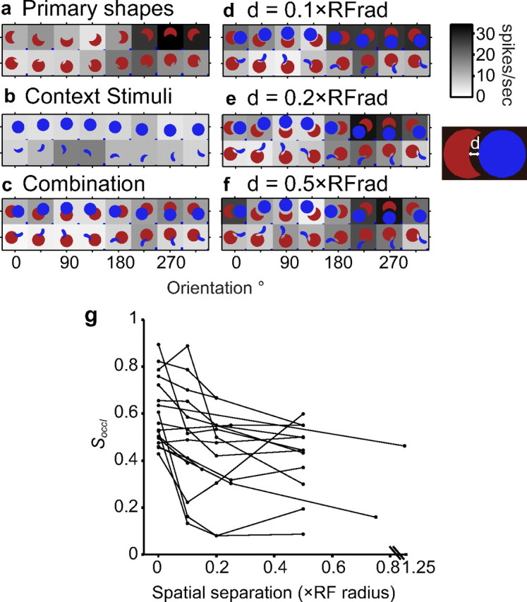
Spatial separation results: example and population. a–f, Example cell. All conventions as in Figure 3. a, Primary shape responses. This neuron responded preferentially to shapes with a sharp convexity adjoined by a concavity at the bottom. b, Responses to contextual stimuli were uniformly weak. c, Combination responses reflect suppression of preferred primary shape responses under partial occlusion context. d–f, A small spatial separation (d, 0.1 × RF radius; e, 0.2 × RF radius; f, 0.5 × RF radius) between primary and contextual stimuli dramatically decreased suppression. g, Population results. Spatial separation (x-axis) versus fractional suppression (y-axis). Most neurons (14 of 17; see Results) show a negative correlation between fractional suppression and spatial separation. Note for the interrupted x-axis: for one neuron, the maximum separation tested was d = 1.25 × RF radius.

Tricolor junctions and spatial proximity

Yet another hypothesis is that the observed suppression is simply the result of the spatial proximity and alignment of the preferred and nonpreferred color patches and that the contour geometry at the T-junction itself does not play a role. In our stimulus design, all accidental contour features are formed at a tricolor junction with a continuous occluding contour forming the hat of the T-junction. To determine whether a tricolor junction alone, without the continuous occluding contour, was sufficient to suppress responses to preferred sharp convexities, we studied responses to stimuli that were equivalent to the combination stimuli being viewed through a circular aperture (Fig. 2h). In these stimuli, although the tricolor junction is preserved, the occluding contour is truncated. Unlike combination stimuli, tricolor control stimuli evoked responses that were comparable with primary shape responses (Fig. 10a–d) and suppression was significantly less evident (S_occl = 0.64 vs S_tricolor = 0.22). Of the 11 cells tested on the tricolor control, 10 showed statistically significant (p < 0.05) lower suppression for the tricolor control stimuli (Fig. 10e). This suggests that a tricolor junction alone is not sufficient and that the continuous occluding contour (the hat of the T-junction) may be necessary for suppressed responses. To further address this point, we quantified the fractional suppression of context stimulus responses (i.e., the foreground or occluding stimulus responses) when presented in combination with primary shapes. Context stimuli spatially adjoin the primary shapes but they lack a curvature discontinuity along their boundary. On 32 cells that showed more than half-maximum responses on at least two context stimuli, we calculated fractional suppression of responses to combination stimuli relative to contextual stimuli. Responses to context stimuli also showed some suppression (average fractional suppression of 0.15) when in combination, but the suppression of contextual responses was significantly less (randomization paired t test, p < 0.01) than suppression of primary shape responses. These results support the hypothesis that spatial proximity alone is not sufficient, and contour geometry, which dictates perception (Chapanis and McCleary, 1953), is likely to be important. Another simple hypothesis is that energy in a specific spatial frequency band underlies the observed suppression. All combination stimuli have a characteristic preferred color/nonpreferred color/preferred color pattern in the stimulus image because of the convex projections in the contextual stimuli. This creates energy in a specific spatial frequency band, and neurons tuned to these spatial frequencies could provide the inhibitory drive to cause the suppression. Such a mechanism will predict identical levels of suppression for preferred contours and their 180° rotated images (attributable to the symmetry of the Fourier transform of real-valued images), but our data demonstrate that this is not the case. For example, compare levels of suppression for stimuli at 270° and 90° in Figure 3. Across all cells, fractional suppression based on preferred stimuli was significantly greater than that based on 180° rotations (average fractional suppression across cells for preferred shapes, 0.32; for 180° rotated shapes, −0.005; randomization t test, p < 0.01). This is despite the fact that suppression for 180° rotated stimuli is biased toward larger values as a result of the low firing rates.

Figure 10.

Results from an example neuron on the tricolor control experiment. All conventions as in Figure 3. a, Primary shape responses. This neuron responded preferentially to primary shapes in the 180°-315° orientations. b, Combination responses revealed strong suppression of preferred primary shape responses (S_occl = 0.64) under partial occlusion context. c, Tricolor control stimuli are visually equivalent to the combination stimuli viewed through a circular aperture. Responses were comparable with primary shape responses (S_tricolor = 0.22). Specifically, responses were not as suppressed as in b. d, Scatter plot of primary shape responses (x-axis) versus combination and tricolor responses (y-axis). Tricolor responses were better correlated with primary shape responses than combination responses. e, Population results for all 11 neurons tested on the tricolor control. Each line represents a cell. y-Axis plots fractional suppression based on combination (left) and tricolor stimuli (right).

Latency of suppression onset

Suppressed encoding of accidental contours emerged soon after response onset. In the example neuron illustrated in Figure 11a–d, onset of suppression is very early, and the timing is comparable with when shape-selective responses appeared, i.e., combination responses (Fig. 11d, blue) and nonpreferred primary responses (Fig. 11d, green) have a similar temporal profile. For this neuron, latency of response onset was 42 ms for preferred primary shapes (Fig. 11a,d, red) and for combination shapes (Fig. 11b,d, blue). The time of suppression onset, which was evaluated as the time at which the difference between the primary responses and combination responses reached statistical significance (see Materials and Methods), was 47 ms. In other words, suppression emerged 5 ms after the onset of preferred primary responses. Across all 76 neurons that showed statistically significant suppression, mean latency for response onset to preferred primary shapes was 55 ms (SD = 25 ms); mean onset latency for combination stimuli was longer (63 ms) and more variable (SD = 49.5 ms). Suppression of combination responses emerged, on average, 13 ms (SD = 25 ms) after the onset of preferred primary responses. To facilitate direct comparison, following Zhou et al. (2000), we quantified the difference histogram (Fig. 11d,e, black) between preferred primary responses and the corresponding combination responses; the time to half-maximum of the difference histogram from stimulus onset was measured as the latency of suppression onset. By this method, latency of suppression onset was 46 ms from stimulus onset for the example in Figure 11a–d and 63 ms for the population (Fig. 11e). This is earlier than the emergence of border ownership signals in V2 (∼68 ms) quantified by the identical method (Zhou et al., 2000).

Discussion

We studied the responses of V4 neurons that were selective for contour curvature to shapes presented in isolation and in the presence of adjoining context to discover which contours of partially occluded objects are encoded. Our results indicate that V4 responses that encode sharp convexities at the T-junction between objects are suppressed by the presence of the contextual stimuli, whereas those encoding broad convex curvatures are essentially unaffected. Hypotheses based on local color, luminance contrasts, and response normalization mechanisms do not explain these results. Control experiments suggest that spatial proximity of the contextual stimulus alone is not sufficient to cause the suppression; the bounding contours of the primary and contextual stimuli need to form a T-junction. Our findings parallel behavioral results that demonstrate longer reaction times when shape matching is based on sharp convex and concave features at the junction between shapes compared with when those features bound a shape in isolation (Rensink and Enns, 1998). These results are also consistent with shape-theoretic and psychophysical results indicating that the sharp convexities at the junction between shapes are perceived as accidental contour features (Helmholtz, 1909; Chapanis and McCleary, 1953). The continuous broad convex curvatures, conversely, are statistically more likely to be real contours even in the presence of adjoining stimuli. Below, we discuss the implications of our findings to the representation of partially occluded objects in V4, the generation of border ownership signals, and the segmentation of images along the ventral stream.

In natural scenes, when objects are partially occluded, the visual system must segment the scene and assign boundaries to the appropriate objects. Shape theorists since the time of Helmholtz (1909) have postulated that T-junctions serve as the primary cue for occlusion (Guzman, 1968; Clowes, 1971; Huffman, 1971; Waltz, 1975). Psychophysical findings also suggest that T-junctions are important for perception under partial occlusion (Elder and Zucker, 1998; Rubin, 2001). In pictorial displays (without depth cues), it is only at T-junctions that the depth ordering of overlapping objects can be determined (Fig. 12a), and, based on this information, the intervening contour can be assigned to the appropriate object (i.e., encoding of border ownership) (Nakayama et al., 1995). Although border ownership signals have been documented in the primate brain (Zhou et al., 2000), it is not known how information at T-junctions leads to their generation. Models of image segmentation and border ownership have typically invoked the explicit or implicit encoding of T-junctions, followed by instantiation of rules to identify the direction of the occluding boundary at the T-junctions (Fig. 12a) (Sajda and Finkel, 1995; Zhaoping, 2005; Craft et al., 2007). Our results provide physiological evidence for how information at T-junctions could influence contour encoding and raises the possibility that the importance of T-junctions could come from the suppression of accidental contours rather than their explicit representation (which has not been physiologically demonstrated). For a complex visual scene with partially occluded objects, suppressed encoding of sharp convexities and concavities at the junction between objects would result in a representation that more strongly encodes the non-accidental real contours of the various objects (Fig. 12c). Such a representation would be equivalent to identifying the direction of the occluding boundary at the T-junction because, once accidental contours are suppressed, the only contour encoded at the T-junction will be the occluding contour. Then, previously proposed collinear and co-circular facilitation mechanisms could lead to appropriate border assignment of the contour away from the T-junctions (Sajda and Finkel, 1995; Zhaoping, 2005; Craft et al., 2007). Preferential encoding of non-accidental contours could also provide an ideal population code for recognition by facilitating the binding together of only those features that are actually associated with an object. Our results suggest that contours of foreground objects are only weakly suppressed by adjoining stimuli, in contrast with a previous study in IT cortex (Missal et al., 1997) that reported much stronger levels of suppression when a second object was presented in the background. This difference may be because their stimuli (∼4.8° in extent at center of gaze) likely activated the suppressive surround of V4 neurons, whereas ours were confined to the V4 RF (see Materials and Methods).

Figure 12.

Summary of border ownership and image segmentation. a, Illustration of border-ownership signals. A V2 neuron (RF illustrated by red circle) may respond strongly when the edge belongs to the object above (left) but not when it belongs to the object below (right), although stimuli are identical within RF. Models of border ownership start with the detection of T-junctions (black circles), followed by the determination of boundary direction (arrows) at the T-junction. b, Summary of tricolor control results and plausible mechanisms. Responses to a sharp convex contour were suppressed when adjoined by a smooth continuous contour (left) but not when adjoined by another sharp convex contour (right). This suggests that the suppressed encoding of accidental contours may be attributable to inhibition from neurons that encode smooth continuous contours at the same RF location. c, Schematic of how a visual scene is encoded in area V4. The first panel shows an example visual scene with partially occluded objects. All contours are present in the retinal image. Real contours are shown in green. Accidental sharp convexities at T-junctions (labeled s) and accidental concavities between the T-junctions (labeled c) are shown in red. The third panel shows the fragmented contour with the accidental sharp convexities (s) suppressed. Co-linear and co-circular facilitation mechanisms may then lead to the suppression of the accidental concavities (c) and the development of border ownership signals (right).

Our results are also consistent with latency results from V2 suggesting that border ownership signals may arise in higher visual areas such as V4. In the experiments demonstrating border-ownership signals (Zhou et al., 2000), because the informative T-junctions were well outside the RF (Fig. 12a) and because the border-ownership signals emerged ∼25 ms after response onset (∼68 from stimulus onset), the authors hypothesized that such signals likely originate in higher visual areas rather than from processing based on long-range connections within V2 (Craft et al., 2007) (but see Zhaoping, 2005). A similar argument based on relative latencies in V2 and V4 has been used to suggest that selectivity for kinetic contours in V2 may result from feedback signals from V4 (Mysore et al., 2006). Pending direct comparisons based on identical stimuli, experimental, and analytical methods, our results suggest that suppression of accidental contours appear early enough in V4 to precede, and perhaps underlie, the generation of border-ownership signals in V2. Thus, our results support previous predictions that V4 plays an important role in image segmentation (Grossberg, 1994) and suggest that suppression of accidental contours could mark the first step of image segmentation in the ventral stream.

Our results are consistent with the hypothesis that local competition between two contours—a sharp convexity and a smooth continuous contour—at the same location in the visual scene produces the observed suppression. When the competition is between two sharp convexities (as in the tricolor junction control) (Fig. 12b), strong suppression is not evident. This could be achieved, for instance, if broad convexity-tuned neurons inhibit sharp convexity-tuned neurons that share a subset of the same V1 inputs. Alternatively, more global processing across a network of neurons, a network-based probabilistic inference (Baek and Sajda, 2005), could underlie these results. Many computer vision algorithms rely on rapid grouping of contour fragments based on principles of cotermination, smoothness, length, convexity, etc., for the completion of occluded objects and detection of salient images in scenes (Lowe, 1985; Sha'ashua and Ullman, 1988; Sporns et al., 1991; Elder and Zucker, 1996; Jacobs, 1996; Supèr et al., 2010). Such groupings are unlikely to include sharp convexities at T-junctions and suppression could result if inclusion in a contour grouping is necessary for the maintenance of strong encoding. Because there is a one-to-one correspondence between local contour geometry and global percepts in our stimulus design, i.e., T-junctions always implied partial occlusion, our results cannot differentiate between local versus global mechanisms. However, because the response suppression reported here emerges much earlier than mean onset latencies in IT cortex [∼93–118 ms depending on the specific stimuli and analytical methods (Kovács et al., 1995; Kiani et al., 2005; Brincat and Connor, 2006)], we hypothesize that the observed effects are the result of computations local to V4 and are unlikely to be attributable to feedback from IT cortex. This, in principle, supports computational models of figure–ground segregation and generation of border ownership implemented without feedback (Sporns et al., 1991; Zhaoping, 2005; Supèr et al., 2010).

Our results cannot be explained in terms of previously proposed models of biased competition that describe how attention modulates responses when multiple stimuli compete within a receptive field (Desimone and Duncan, 1995; Reynolds et al., 1999). When contextual and primary stimuli are presented in combination, if attention is consistently directed to the contextual stimulus, suppression of primary shape responses could occur. However, this cannot explain the systematic relationship we observed between the extent of suppression and the tuning preference of cells (Fig. 6), nor can it explain the lack of suppression when the primary and contextual stimulus locations are interchanged (swapped location control). Although our experiment did not explicitly control for attention, our stimuli were carefully designed to avoid automatic attentional selection of one of the stimuli based on color, luminance contrast, or stimulus area. Finally, the animals were not trained on any behavior other than simple fixation.

Given the limited time in our recording preparation and the high-dimensional stimulus sets related to compound stimuli, our study focused on one specific case of partial occlusion: when occlusion results in T-junctions with sharp convex accidental contour features. In natural vision, however, occlusion takes a myriad of other forms, for example, (i) when the occluding and occluded object contours do not intersect, such as when a smaller disk is in front of a larger disk, (2) when concave occluders produce accidental broad convexities, and (3) when occluders extend outside the V4 RF. These cases were not investigated here, nor were depth cues, da Vinci stereopsis (Nakayama et al., 1989), and surface properties (Grossberg, 1994; Nakayama et al., 1995), all of which are known to contribute to the processing of occlusion and image segmentation, and need to be investigated to fully understand the neural representation of visual occlusion.

References

- Albright TD, Stoner GR. Contextual influences on visual processing. Annu Rev Neurosci. 2002;25:339–379. doi: 10.1146/annurev.neuro.25.112701.142900. [DOI] [PubMed] [Google Scholar]
- Baek K, Sajda P. Inferring figure-ground using a recurrent integrate-and-fire neural circuit. IEEE Trans Neural Syst Rehabil Eng. 2005;13:125–130. doi: 10.1109/TNSRE.2005.847388. [DOI] [PubMed] [Google Scholar]
- Bakin JS, Nakayama K, Gilbert CD. Visual responses in monkey areas V1 and V2 to three-dimensional surface configurations. J Neurosci. 2000;20:8188–8198. doi: 10.1523/JNEUROSCI.20-21-08188.2000. [DOI] [PMC free article] [PubMed] [Google Scholar]
- Brincat SL, Connor CE. Dynamic shape synthesis in posterior inferotemporal cortex. Neuron. 2006;49:17–24. doi: 10.1016/j.neuron.2005.11.026. [DOI] [PubMed] [Google Scholar]
- Chapanis A, McCleary RA. Interposition as a cue for the perception of relative distance. J Gen Psychol. 1953;48:113–132. [Google Scholar]
- Clowes MB. On seeing things. Artif Intell. 1971;17:79–116. [Google Scholar]
- Craft E, Schütze H, Niebur E, von der Heydt R. A neural model of figure-ground organization. J Neurophysiol. 2007;97:4310–4326. doi: 10.1152/jn.00203.2007. [DOI] [PubMed] [Google Scholar]
- Desimone R, Duncan J. Neural mechanisms of selective visual attention. Annu Rev Neurosci. 1995;18:193–222. doi: 10.1146/annurev.ne.18.030195.001205. [DOI] [PubMed] [Google Scholar]
- de Wit TC, Bauer M, Oostenveld R, Fries P, van Lier R. Cortical responses to contextual influences in amodal completion. Neuroimage. 2006;32:1815–1825. doi: 10.1016/j.neuroimage.2006.05.008. [DOI] [PubMed] [Google Scholar]
- Elder JH, Zucker SW. Computing contour closure. Presented at the Fourth European Conference on Computer Vision; April 14–18; Cambridge, UK. 1996. [Google Scholar]
- Elder JH, Zucker SW. Evidence for boundary-specific grouping. Vision Res. 1998;38:143–152. doi: 10.1016/s0042-6989(97)00138-7. [DOI] [PubMed] [Google Scholar]
- Fallah M, Stoner GR, Reynolds JH. Stimulus-specific competitive selection in macaque extrastriate visual area V4. Proc Natl Acad Sci U S A. 2007;104:4165–4169. doi: 10.1073/pnas.0611722104. [DOI] [PMC free article] [PubMed] [Google Scholar]
- Gattass R, Sousa AP, Gross CG. Visuotopic organization and extent of V3 and V4 of the macaque. J Neurosci. 1988;8:1831–1845. doi: 10.1523/JNEUROSCI.08-06-01831.1988. [DOI] [PMC free article] [PubMed] [Google Scholar]
- Gawne TJ, Martin JM. Responses of primate visual cortical V4 neurons to simultaneously presented stimuli. J Neurophysiol. 2002;88:1128–1135. doi: 10.1152/jn.2002.88.3.1128. [DOI] [PubMed] [Google Scholar]
- Gerbino W, Salmaso D. The effect of a modal completion on visual matching. Acta Psychol (Amst) 1987;65:25–46. doi: 10.1016/0001-6918(87)90045-x. [DOI] [PubMed] [Google Scholar]
- Grossberg S. 3-D vision and figure-ground separation by visual cortex. Percept Psychophys. 1994;55:48–121. doi: 10.3758/bf03206880. [DOI] [PubMed] [Google Scholar]
- Guzman A. Fall joint computer conference. Arlington, VA: American Federation of Information Processing Societies; 1968. Decomposition of a visual scene into three-dimensional bodies; pp. 291–304. [Google Scholar]
- Helmholtz H. Treatise on physiological optics. New York: Dover; 1909. [Google Scholar]
- Huffman DA. Impossible objects as nonsense sentences. Mach Intell. 1971;5:295–323. [Google Scholar]
- Jacobs DW. Robust and efficient detection of salient convex groups. IEEE Trans Pattern Anal Mach Intell. 1996;18:23–37. [Google Scholar]
- Kiani R, Esteky H, Tanaka K. Differences in onset latency of macaque inferotemporal neural responses to primate and non-primate faces. J Neurophysiol. 2005;94:1587–1596. doi: 10.1152/jn.00540.2004. [DOI] [PubMed] [Google Scholar]
- Kourtzi Z, Kanwisher N. Representation of perceived object shape by the human lateral occipital complex. Science. 2001;293:1506–1509. doi: 10.1126/science.1061133. [DOI] [PubMed] [Google Scholar]
- Kovács G, Vogels R, Orban GA. Selectivity of macaque inferior temporal neurons for partially occluded shapes. J Neurosci. 1995;15:1984–1997. doi: 10.1523/JNEUROSCI.15-03-01984.1995. [DOI] [PMC free article] [PubMed] [Google Scholar]
- Lerner Y, Harel M, Malach R. Rapid completion effects in human high-order visual areas. Neuroimage. 2004;21:516–526. doi: 10.1016/j.neuroimage.2003.08.046. [DOI] [PubMed] [Google Scholar]
- Lowe DW. Perceptual organizqation and visual recognition. Boston: Kluwer Academic; 1985. [Google Scholar]
- Manly BFJ. Randomization, bootstrap and Monte Carlo methods in biology. Ed 2. Boca Raton, FL: Chapman and Hall/CRC; 1997. [Google Scholar]
- McDermott J, Adelson EH. The geometry of the occluding contour and its effect on motion interpretation. J Vis. 2004;4:944–954. doi: 10.1167/4.10.9. [DOI] [PubMed] [Google Scholar]
- Missal M, Vogels R, Orban GA. Responses of macaque inferior temporal neurons to overlapping shapes. Cereb Cortex. 1997;7:758–767. doi: 10.1093/cercor/7.8.758. [DOI] [PubMed] [Google Scholar]
- Murray MM, Imber ML, Javitt DC, Foxe JJ. Boundary completion is automatic and dissociable from shape discrimination. J Neurosci. 2006;26:12043–12054. doi: 10.1523/JNEUROSCI.3225-06.2006. [DOI] [PMC free article] [PubMed] [Google Scholar]
- Mysore SG, Vogels R, Raiguel SE, Orban GA. Processing of kinetic boundaries in macaque V4. J Neurophysiol. 2006;95:1864–1880. doi: 10.1152/jn.00627.2005. [DOI] [PubMed] [Google Scholar]
- Nakayama K, Shimojo S, Silverman GH. Stereoscopic depth: its relation to image segmentation, grouping, and the recognition of occluded objects. Perception. 1989;18:55–68. doi: 10.1068/p180055. [DOI] [PubMed] [Google Scholar]
- Nakayama K, He Z, Shimojo S. Visual surface representation: a critical link between lower-level and higher-level vision. In: Kosslyn SM, Osherson DN, editors. An invitation to cognitive sciences. Cambridge, MA: Massachusetts Institute of Technology; 1995. pp. 1–70. [Google Scholar]
- Pasupathy A, Connor CE. Responses to contour features in macaque area V4. J Neurophysiol. 1999;82:2490–2502. doi: 10.1152/jn.1999.82.5.2490. [DOI] [PubMed] [Google Scholar]
- Pasupathy A, Connor CE. Shape representation in area V4: position-specific tuning for boundary conformation. J Neurophysiol. 2001;86:2505–2519. doi: 10.1152/jn.2001.86.5.2505. [DOI] [PubMed] [Google Scholar]
- Pasupathy A, Connor CE. Population coding of shape in area V4. Nat Neurosci. 2002;5:1332–1338. doi: 10.1038/nn972. [DOI] [PubMed] [Google Scholar]
- Rauschenberger R, Liu T, Slotnick SD, Yantis S. Temporally unfolding neural representation of pictorial occlusion. Psychol Sci. 2006;17:358–364. doi: 10.1111/j.1467-9280.2006.01711.x. [DOI] [PubMed] [Google Scholar]
- Rensink RA, Enns JT. Early completion of occluded objects. Vision Res. 1998;38:2489–2505. doi: 10.1016/s0042-6989(98)00051-0. [DOI] [PubMed] [Google Scholar]
- Reynolds JH, Chelazzi L, Desimone R. Competitive mechanisms subserve attention in macaque areas V2 and V4. J Neurosci. 1999;19:1736–1753. doi: 10.1523/JNEUROSCI.19-05-01736.1999. [DOI] [PMC free article] [PubMed] [Google Scholar]
- Rubin N. The role of junctions in surface completion and contour matching. Perception. 2001;30:339–366. doi: 10.1068/p3173. [DOI] [PubMed] [Google Scholar]
- Sajda P, Finkel LH. Intermediate-level visual representations and the construction of surface perception. J Cogn Neurosci. 1995;7:267–291. doi: 10.1162/jocn.1995.7.2.267. [DOI] [PubMed] [Google Scholar]
- Sha'ashua A, Ullman S. The detection of globally salient structures using a locally connected network. Presented at the Second IEEE Conference on Computer Vision; Dec 5–8; Tarpon Springs, Florida. 1988. [Google Scholar]
- Sporns O, Tononi G, Edelman GM. Modeling perceptual grouping and figure-ground segregation by means of active reentrant connections. Proc Natl Acad Sci U S A. 1991;88:129–133. doi: 10.1073/pnas.88.1.129. [DOI] [PMC free article] [PubMed] [Google Scholar]
- Sugita Y. Grouping of image fragments in primary visual cortex. Nature. 1999;401:269–272. doi: 10.1038/45785. [DOI] [PubMed] [Google Scholar]
- Supèr H, Romeo A, Keil M. Feed-forward segmentation of figure-ground and assignment of border-ownership. PLoS One. 2010;5:e10705. doi: 10.1371/journal.pone.0010705. [DOI] [PMC free article] [PubMed] [Google Scholar]
- Waltz DL. Understanding line drawings of scenes with shadows. In: Winston PH, editor. The psychology of computer vision. New York: McGraw Hill; 1975. [Google Scholar]
- Zhaoping L. Border ownership from intracortical interactions in visual area v2. Neuron. 2005;47:143–153. doi: 10.1016/j.neuron.2005.04.005. [DOI] [PubMed] [Google Scholar]
- Zhou H, Friedman HS, von der Heydt R. Coding of border ownership in monkey visual cortex. J Neurosci. 2000;20:6594–6611. doi: 10.1523/JNEUROSCI.20-17-06594.2000. [DOI] [PMC free article] [PubMed] [Google Scholar]
- Zoccolan D, Cox DD, DiCarlo JJ. Multiple object response normalization in monkey inferotemporal cortex. J Neurosci. 2005;25:8150–8164. doi: 10.1523/JNEUROSCI.2058-05.2005. [DOI] [PMC free article] [PubMed] [Google Scholar]