qCSF in Clinical Application: Efficient Characterization and Classification of Contrast Sensitivity Functions in Amblyopia

The qCSF provides efficient characterization and classification of contrast sensitivity functions in amblyopia.

Abstract

Purpose.

The qCSF method is a novel procedure for rapid measurement of spatial contrast sensitivity functions (CSFs). It combines Bayesian adaptive inference with a trial-to-trial information gain strategy, to directly estimate four parameters defining the observer's CSF. In the present study, the suitability of the qCSF method for clinical application was examined.

Methods.

The qCSF method was applied to rapidly assess spatial CSFs in 10 normal and 8 amblyopic participants. The qCSF was evaluated for accuracy, precision, test–retest reliability, suitability of CSF model assumptions, and accuracy of amblyopia screening.

Results.

qCSF estimates obtained with as few as 50 trials matched those obtained with 300 Ψ trials. The precision of qCSF estimates obtained with 120 and 130 trials, in normal subjects and amblyopes, matched the precision of 300 Ψ trials. For both groups and both methods, test–retest sensitivity estimates were well matched (all R > 0.94). The qCSF model assumptions were valid for 8 of 10 normal participants and all amblyopic participants. Measures of the area under log CSF (AULCSF) and the cutoff spatial frequency (cutSF) were lower in the amblyopia group; these differences were captured within 50 qCSF trials. Amblyopia was detected at an approximately 80% correct rate in 50 trials, when a logistic regression model was used with AULCSF and cutSF as predictors.

Conclusions.

The qCSF method is sufficiently rapid, accurate, and precise in measuring CSFs in normal and amblyopic persons. It has great potential for clinical practice.

Amblyopia is a developmental visual disorder characterized by poor spatial vision without detectable structural or pathologic abnormalities.^1,2 It affects 2% to 4% of the general population² and is the most common cause of uniocular blindness in adults.³ In the United States, 750,000 preschoolers are at risk for amblyopia, and roughly half of those may not be identified before school age.⁴ In China, it is believed that there are tens of millions of children affected by the visual disorder.⁵ Amblyopia has become a serious social and economic challenge.⁶

Amblyopia impairs visual functions, which include but are not limited to visual letter acuity, grating acuity, contrast sensitivity,^7,8 contour integration,^9–11 and global motion perception.^12,13 Of these functions, it is letter acuity, measured rapidly with a chart and easy to understand, that is widely used in screening, early intervention, and treatment evaluation of amblyopia. However, it has been suggested that the contrast sensitivity function (CSF), which describes how visual sensitivity varies as a function of grating spatial frequency, characterizes amblyopia's spatial vision deficits better than does letter acuity.^14–25 For example, contrast sensitivity at high spatial frequencies is still abnormal in amblyopes who are deemed “treated” based on the criterion of remediated visual acuity.²⁶ CSF testing could improve screening, diagnosis, and evaluation of treatment outcomes of amblyopia.

Current clinical CSF tests typically use preprinted letter/grating charts such as the Vistech contrast sensitivity chart (Vistech, Hartford, CT), the Functional Acuity Contrast Test (FACT), the Pelli-Robson chart,^27,28 and the CVS-1000 series chart (VectorVision, Greenville, OH). Although chart tests are convenient in clinical use, their limited number of contrast levels greatly limits the range and resolution of the test grating stimuli.^29–33 In addition, charts using broadband letters as stimuli (e.g., the Pelli-Robson chart), are typically insensitive to frequency-specific deficits.³⁴ In contrast, the CSF can be measured with higher precision and accuracy in laboratory psychophysical tests. However, even with adaptive methods such as the QUEST³⁵ or Ψ method,³⁶ a reasonable threshold estimate at a single spatial frequency usually takes 50 to 100 trials. Consequently, a CSF measurement obtained with conventional adaptive methods, sampling at seven different spatial frequencies, requires up to 700 trials, can take 1 hour, and is therefore too time-consuming, making it unsuitable for clinical use.

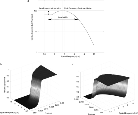
Lesmes et al.³⁷ recently developed a novel adaptive psychophysical procedure, the qCSF method, which estimates the full CSF rapidly (∼5–10 minutes) with reasonable precision (2–3 dB). (In this paper, 1 dB = 0.05 log units, 12%; but in the clinical definition of decibels [1 dB = 0.1 log units], the precision and bias were half of the corresponding estimates.) The method applies a Bayesian adaptive test strategy, first developed to estimate the threshold and slope of psychometric functions,^36,38 to directly estimate CSF parameters. The CSF form assumed by the qCSF is the truncated log-parabola,^39,40 which is specified by four parameters: (1) the peak gain (sensitivity), γ_max; (2) the peak spatial frequency ƒ_max; (3) the bandwidth β, which describes the function's full-width at half-maximum (in octaves); and (4) δ, the low-frequency truncation level (Fig. 1). Lesmes et al.³⁷ validated the qCSF method with a psychophysical experiment, using an orientation identification task in three normal subjects. Combined with simulation results, they demonstrated that 50 to 100 qCSF trials provided accurate CSF estimates.

Figure 1.

(a) The classic CSF function, representing how contrast thresholds vary with grating frequency, is typically represented at a single performance level (e.g., 75% correct in a 2AFC task). Here, the CSF's shape is defined by a truncated log-parabola using four parameters. This CSF represents a horizontal cross-section through a psychometric surface (b), which describes percent correct as a bi-variate function of grating contrast and spatial frequency. For the sake of simplifying CSF estimation, the qCSF assumes this functional form and that the transition from minimum to maximum asymptote (which depends on psychometric slope) is equally steep at all spatial frequencies. (c) The psychometric surface from a different viewing angle (rotated 90° on the z-axis).

The testing time savings provided by the qCSF comes from (1) assuming a CSF model and (2) using an efficient Bayesian test strategy to estimate the model's free parameters. Briefly, the qCSF model assumes that the observer's CSF can be described by using a functional form, the truncated log-parabola, with four free parameters. The model also assumes that other parameters underlying psychophysical performance, such as the slope of the psychometric function or the lapse rate,^41–43 are fixed. After defining a probability distribution over the four CSF parameters, a one-step-ahead search of the stimulus space (over dimensions of spatial frequency and contrast) is used to choose stimuli that maximize the information gained over the CSF parameter space.^36,38,44,45 After the Bayesian update of the probability distribution following each trial, a CSF estimate can be calculated from the expected values of the four parameters.

Despite the great advantages of the qCSF, a model-dependent test strategy poses risks. Model mismatch, between the fixed parameters of the assumed qCSF model and the empirical model presented by the observer, can introduce systematic bias into estimates of the parameters. This risk is especially salient for clinical applications, in which visual disease may introduce model mismatch, by affecting all CSF model parameters, fixed or free. In this study, we evaluated the qCSF's potential as a clinical CSF assessment procedure by applying it to the measurement of contrast sensitivity functions in normal and amblyopic populations. For independent CSF assessment in amblyopic and normal subjects, we interleaved qCSF assessment with an independent adaptive procedure, the Ψ method.³⁶ Such an independent assessment was critical for evaluating the relative accuracy of qCSF estimates, in addition to the accuracy of several model assumptions: (1) Individual CSFs can be well described with a specific functional form; and (2) the slopes of psychometric functions at different spatial frequencies are the same. These assumptions, which allow CSF task performance to be modeled as a relatively simple psychometric surface (Fig. 1), have support in the empiric literature on CSFs in the normal population.^39,40,46 However, they must be re-evaluated in clinical populations.

We report that the qCSF method required only 100 trials (5–10 minutes) to provide CSF estimates with a precision (1 SD) of 2.6 dB for normal subjects and 3.2 dB for amblyopes. Moreover, CSF features estimated by 50 qCSF trials distinguished normal subjects and amblyopes with an accuracy of approximately 80%. Furthermore, the assumptions used in the qCSF were valid in 8 of 10 normal participants and in all amblyopic participants. Taken together, the findings in our study indicate that the qCSF method provides efficient CSF measurements in both normal and amblyopic populations and competent performance for early screening and treatment evaluation in amblyopia clinical practice.

Methods

Subjects

Ten normal subjects (N1–N10) aged from 21 to 24 years (mean, 21.6 ± 1.6 years) and eight amblyopes (A1–A8) aged from 20 to 31 years (mean, 23.3 ± 3.7 years) participated in the experiments. All subjects were naïve to the purpose of the experiment. All normal subjects had normal or corrected-to-normal vision and no prior experience in psychophysical experiments. The amblyopes were diagnosed by two ophthalmologists (LF and LT). Six of them had participated in other psychophysical experiments. The detailed characteristics of the amblyopia group are listed in Table 1. The research adhered to the tenets of the Declaration of Helsinki. Written informed consent was obtained from the subjects after explanation of the nature and possible consequences of the study. The experiments were conducted according to the experimental protocol for human subjects approved by the ethics committee (IRB) of the School of Life Science, University of Science and Technology of China.

Table 1.

Characteristics of Each Amblyopic Participant

No.	Sex	Age (y)	Eye	Type of Amblyopia	Eye Alignment	Correction	Acuity	Test-Retest Interval (d)	Experienced
1	M	20	AE	Anisometropia	None	1.50DC×90	2.5	1	Yes
			FE			−1.50DS:0.75DC×180°	1.0
2	M	25	AE	Strabismus/anisometropia	RXT 10Δ	0.75DS	10.0	5	Yes
			FE			−5.00DS	1.3
3	F	20	AE	Anisometropia	None	+3.00DS:+1.00DC×15°	2.0	12	Yes
			FE			+0.50DS:+0.50DC×160°	1.3
4	F	22	AE	Anisometropia	None	+2.50DS	2.0	15	Yes
			FE			Plano	1.0
5	M	31	AE/LE/Measured	Anisometropia	None	+4.00DS	2.5	4	No
			AE/RE		None	+5.00DS	2.0
6	M	22	AE/RE/Measured	Anisometropia	None	+6.00DS	4.0	3	Yes
			AE/LE		None	+3.00DS	1.3
7	M	21	AE	Strabismus/anisometropia	LET 10Δ	+1.25DS:+0.50DC×180°	5.0	12	Yes
			FE			+1.00DS	0.67
8	M	25	AE	Strabismus/anisometropia	LET 18Δ	6.50DS:+1.00DC×80°	5.0	7	No
			FE			5.50DS	1.3

Acuity is expressed in minimum angle of resolution (MAR). AE: amblyopic eye, FE: fellow eye; LE: left eye, RE: right eye.

Apparatus

The stimuli were displayed on a computer monitor, driven by a video card (model G220 monitor; Sony, Tokyo, Japan, and 9250 ATI Radeon video card; AMD, Sunnyvale, CA). The monitor had a display area of 32.8 × 24.4 cm, a resolution of 1024 × 768, and a refresh rate of 100 Hz. The mean luminance of the display was 34 cd/m². A special circuit was used to achieve 14-bit grayscale resolution.⁴⁷ Stimuli were generated on the fly by a technical computing software (MatLab 7.1.0.14; The MathWorks Corp., Natick, MA) and Psychtoolbox subroutines.^48,49 Participants viewed the stimuli monocularly at a distance of 2.4 m. A chin–forehead-rest was used to minimize head movements during the experiment.

Stimuli

The stimuli were static vertical sinusoidal gratings with a size of 3.0° × 3.0°. A spatial envelope (0.5° half-Gaussian) was used to blend the grating's edge into the background, resulting in a 2.0° × 2.0° patch with full contrast.

qCSF Implementation

As mentioned earlier, in the qCSF procedure, the CSF is described by a truncated log-parabola with four parameters: (1) the peak gain (sensitivity), γ_max; (2) the peak spatial frequency ƒ_max; (3) the bandwidth β, which describes the function's full-width at half-maximum (in octaves), and (4) δ, the low-frequency truncation level. The possible CSFs considered for Bayesian inference were represented by a probability distribution over a gridded parameter space, T_ν→, where ν→ = (γ_max, f_max, β, δ). The stimulus space, T_x→, where x→ = (c, f), represents all possible grating stimuli with contrast c and spatial frequency f. The goal of the qCSF method is to efficiently search the stimulus space to gain information in the parameter space. See Appendix A for a more detailed description of the qCSF algorithm.

Parameter Settings

For the qCSF method, the stimulus space x→ = (c, f) comprises gratings that vary in contrast (from 0.1%–99% in 1.5-dB steps) and spatial frequency (from 0.5 to 16 cycles per degree [cpd] in 3-dB steps). One exception was observer A1, who was tested at spatial frequencies that varied from 0.5 to 12 cpd in 3-dB steps, based on practice results. For the Ψ method, stimulus contrast c was sampled from 0.1% to 99% in 1-dB steps; contrast thresholds were measured independently at 0.69, 1.29, 2.42, 4.54, 8.52, and 16.00 cpd for all subjects except A1. For subject A1, thresholds were measured at 0.67, 1.19, 2.12, 3.78, 6.73, and 12.00 cpd.

A log-Weibull psychometric function was adopted for both the qCSF and Ψ procedures

where τ is the to-be-measured contrast threshold, and the other parameters were fixed: Chance performance rate γ was set to 0.5, the lapse rate λ was set to 0.04, and the psychometric slope η was set to 3.5. (The value of 3.5 was based on its use in the QUEST method.³⁵ The Discussion section presents simulation results that demonstrate that matching the assumed slope and the observer's slope is not critical for threshold estimation.) For the qCSF, the threshold variable, τ, was defined by the CSF model. For the Ψ method, τ was estimated independently at each spatial frequency.

Procedure

A two-interval, forced-choice (2IFC) grating detection task was used. In each trial, a grating was randomly presented in one of two successive intervals. The intervals were separated by 500 ms, with a brief tone signaling each interval's onset. In both intervals, a 120-ms presentation of the grating stimulus or a blank screen was preceded by a cross-hair frame (250 ms) that aided stimulus localization and fixation. Participants were asked to indicate which interval contained the grating. A new trial started 500 ms after the subject's response. No feedback was provided.

Design

One hundred practice trials were used to familiarize each participant with the task. Both the qCSF and Ψ methods were used to estimate CSFs from the dominant eye of normal participants and the amblyopic eye of each amblyopic participant (or the worse eye in subjects with binocular amblyopia). For CSF measures obtained with the Ψ method,³⁶ contrast thresholds were estimated independently at six spatial frequencies with 50 trials for each spatial frequency and a total of 300 trials. A qCSF run encompassed 300 trials. To compare the results from the qCSF and Ψ methods, contrast thresholds obtained with the qCSF method were calculated at the six spatial frequencies used in the Ψ method. All participants completed two sessions of 600 trials, with 300 qCSF trials randomly intermixed with 300 Ψ trials. Because of scheduling conflicts, the interval between the two sessions ranged from 1 to 15 days across subjects (see Table 1 for details).

Results

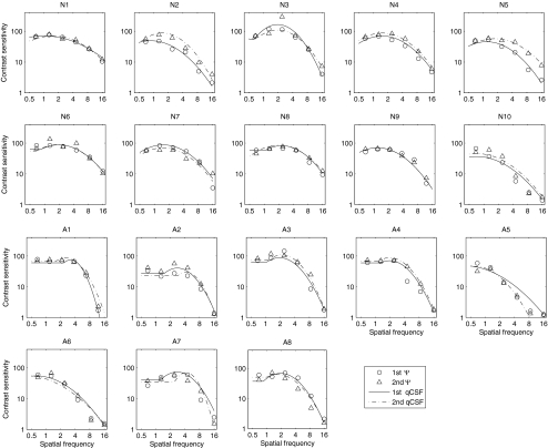
Figure 2 shows plots of CSFs estimated with both the Ψ and qCSF methods. In the following sections, we evaluate the precision and accuracy of qCSF estimates, examine the test–retest reliability of both CSF testing methods, and check qCSF model assumptions. We also evaluate the potential of qCSF in amblyopia screening, by testing how well CSF features estimated with the qCSF can predict membership in the two groups.

Figure 2.

For each participant, CSFs obtained with the qCSF and Ψ methods in each of two sessions are plotted. N1 to N10 represent 10 normal participants, and A1 to A8 represent 8 amblyopic participants. Circles: estimates of contrast sensitivities using the Ψ method in the first session. Triangles: estimates of contrast sensitivities using the Ψ method in the second session. Continuous curves: estimates of the CSF curve using the qCSF method in the first session. Dotted curves: estimates of the CSF curves using the qCSF method in the second session. The triangle at 16 cpd in A5 was excluded from the analysis because the measurement was unreliable.

Precision

The precision of CSF estimates obtained with the qCSF and Ψ methods was estimated through a bootstrap procedure⁵⁰ based on 500 simulated repetitions of full experimental runs of 300 qCSF and 300 Ψ trials. For each participant, the slope of the psychometric functions was assumed to be the slope of the best-fitting single-slope Weibull function (see Assumptions Check). For each observer, the precision in a qCSF or Ψ run was characterized by the standard deviation of the distribution of resampled threshold estimates:

where k indexes spatial frequency, i indexes repetition, and τ^k is the mean threshold of N repetitions in the kth spatial frequency condition.

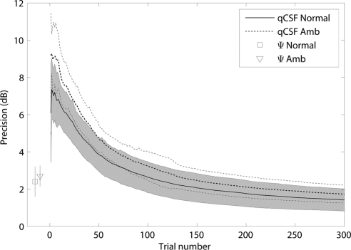
The precision of the qCSF method for each participant in each session was calculated trial by trial. There was no significant difference between two sessions for both groups (for 78.3% trials of the normal group and all trials of amblyopia group [P > 0.10, paired t-test], but for all trials of the normal group [P > 0.05; paired t-test]). The averaged precision of the qCSF method over participants and sessions for both the normal and amblyopia groups are shown in Figure 3 as a function of the number of trials. The average precision of the normal group was 3.86 ± 0.91, 2.63 ± 0.83, and 1.41 ± 0.59 dB after 50, 100, and 300 qCSF trials, respectively. The average precision of the amblyopia group was 4.71 ± 0.74, 3.23 ± 0.77, and 1.73 ± 0.48 dB after 50, 100, and 300 qCSF trials. The standard deviations in the amblyopia group were larger than those in the normal group until the 110th trial (for any trial before 110, P < 0.05; t-test). The average precision of the Ψ method for the normal and amblyopia groups was 2.40 ± 0.80 and 2.70 ± 0.55 dB, respectively, in 300 trials. The precision achieved with ∼120 qCSF trials matched that obtained with 300 Ψ trials in the normal group. The precision achieved with ∼130 qCSF trials matched that obtained with 300 Ψ trials in the amblyopia group.

Figure 3.

The average precision of the qCSF method as a function of the number of trials. The average precision of the Ψ method for both groups are marked. The error bar represents 1 SD. The curves represent the normal and amblyopia groups. The shaded region represents the variability of 1 SD for the normal group. The thin dotted lines indicate the variability (±1 SD) for the amblyopic group.

Bias

To evaluate the relative bias of qCSF estimates, we derived qCSF threshold estimates for the six spatial frequencies used in the Ψ method and compared them with those directly estimated by the Ψ method. The bias was defined as the difference between the thresholds obtained by the qCSF and Ψ methods:

where k indexes spatial frequency, and log(τ_Ψ^k) is the average threshold from the two sessions.

The average bias of all participants in each group was computed as

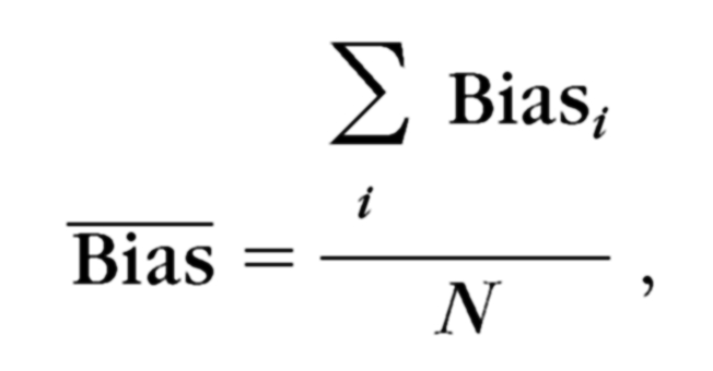where i is the index of each participant. The SD of the bias was computed as

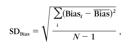where N is the number of participants in each group.

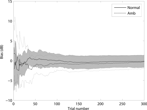
The trial-by-trial bias was calculated for each subject in each session. There was no significant difference between the two sessions in both groups (99.7% for the normal group and 99.3% for the amblyopia group, P > 0.10; paired t-test). The average bias over the two sessions is plotted as a function of the number of trials for the normal and amblyopia groups in Figure 4. Averaged over sessions, the mean bias of the qCSF method after 50, 100, and 300 trials was 0.32, −0.03, and −0.16 dB in the normal group, and −1.38, −0.78, and −0.24 dB in the amblyopia group. For both groups, these biases were not significantly different from 0 (P > 0.10; t-test).

Figure 4.

Relative bias estimates of the qCSF method, shown as a function of trial number. The shaded region represents the variability (±1 SD) of bias estimates for the normal group. The thin dotted lines indicate the variability (±1 SD) for the amblyopic group.

Test–Retest Reliability

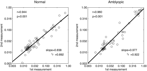
For both normal and amblyopic subjects, the test–retest reliability of CSF measures obtained with the qCSF and Ψ methods was evaluated. For both methods, we calculated the Pearson correlation between log thresholds measured in the first and second sessions, at six different frequencies. The test–retest correlations for the Ψ method were 0.944 and 0.960 (both P < 0.001) for the normal and amblyopia groups, respectively (Fig. 5). Linear regression was also applied to analyze thresholds obtained from both groups. The slope for the Ψ method was 0.837 (confidence interval [CI]: 0.761–0.914), with r² = 0.892 in the normal group, and 0.977 (CI: 0.893–1.06), with r² = 0.922 in the amblyopia group.

Figure 5.

The thresholds measured by the Ψ method in the first session were plotted against those measured in the second session. Linear regression was performed to evaluate the test–retest reliability.

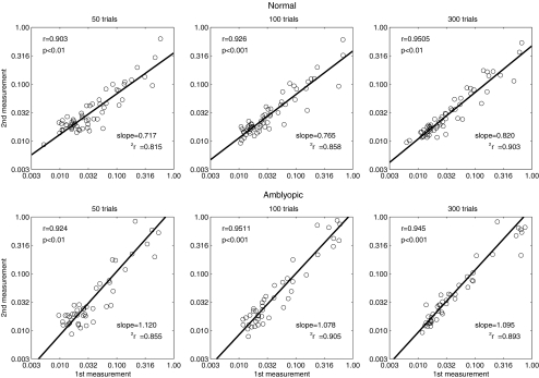
Similar correlation and linear regression analyses were performed on the thresholds obtained by the qCSF method after 50, 100, and 300 trials (Fig. 6). For the normal group, the correlations for the qCSF estimates obtained with 50, 100, and 300 trials were 0.903, 0.926, and 0.951 (all P < 0.001), respectively. For the amblyopia group, the correlations were 0.924, 0.951, and 0.945 (all P < 0.001). For thresholds measured in 50 qCSF trials, the slope of the linear regression between the first and second sessions was 0.717 (CI: 0.627–0.806, r² = 0.815) in the normal group, and 1.12 (CI: 0.983–1.26, r² = 0.855) in the amblyopia group. After 100 qCSF trials, the slopes in the normal and amblyopia groups were 0.765 (CI: 0.683–0.847, r² = 0.858) and 1.078 (CI: 0.975–1.18, r² = 0.905). After 300 qCSF trials, the slopes in the normal and amblyopia groups were 0.820 (CI: 0.750–0.891, r² = 0.903) and 1.095 (CI: 0.983–1.21, r² = 0.893), respectively.

Figure 6.

The thresholds measured by the qCSF method in the first session were plotted against those measured in the second session. Linear regression was performed to evaluate the test–retest reliability.

These results showed that, for both groups and both methods, threshold estimates in the two sessions were well matched with as few as 50 qCSF trials.

Assumptions Check

The qCSF method makes several assumptions: (1) that CSF can be described by a truncated log-parabolic function, and (2) that the slope of the psychometric function is invariant across spatial frequencies. Violations of these assumptions could introduce bias and imprecision into the qCSF estimates. We used the CSF data independently obtained with the Ψ method to evaluate the assumptions in turn.

To verify how well the truncated log-parabolic model used by the qCSF can account for the empiric CSF data, we fit the model

to the contrast sensitivities estimated at the six different spatial frequencies used in the Ψ method. Thirty-six sets of CSFs (18 participants in two sessions) measured by the Ψ method were fitted. In the normal group, the mean r² was 0.983 ± 0.014 in the first session and 0.968 ± 0.034 in the second session. In the amblyopia group, the mean r² was 0.955 ± 0.018 and 0.965 ± 0.021 in the first and second sessions, respectively. Consistent with previous reports,³⁹ the truncated log-parabolic model provided an excellent description of the CSFs in the normal group. Our results also suggest that the same functional form can be used to describe CSFs in amblyopic vision.

In addition, we calculated the slope of the psychometric function at each of the six spatial frequencies, using the data obtained by the Ψ method. For each subject, data from the two sessions were pooled. The 100 trials in each spatial frequency condition were binned by dividing the log contrast range into five equal parts. The percentage of correct responses in the five bins allowed us to construct a raw psychometric function for each spatial frequency. The raw psychometric functions were then aligned by transferring the abscissa into a log relative contrast unit^46,51: c′ = log10(contrast) − log10(τ), where τ is the threshold.

We then fit the relative psychometric functions with the Weibull function (equation 1), by using a maximum likelihood procedure^52,53

where i indexes the contrast condition, N_i and K_i are the number of total and correct trials, and P_i is the percentage correct predicted by the Weibull function. A full model with six independent slopes at six different spatial frequencies and a reduced model with a single slope across six different spatial frequencies were compared by using the χ² statistic^52,53

where df = k_full − k_reduced, and k is the number of parameters in each model.

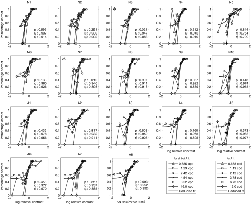
In Figure 7, the raw psychometric functions along with the best-fitting reduced model of each participant were plotted. (Given that the Ψ method places most trials near and above threshold, the number of trials in each bin is unevenly distributed. The lowest bins tend to contain only a few trials [1–5]; this results in the lower-than-chance performance [e.g., 0% correct] evident at the lowest relative contrast levels in Fig. 7.) The result showed that, for 8 of 10 normal and all 8 amblyopic participants, the full and the reduced models provided statistically equivalent fits to the data (P > 0.1). For these subjects, the slope invariance assumption is correct. Averaged over subjects, the best-fitting slope of the reduced model is 1.70 ± 0.53 in the normal group and 1.36 ± 0.32 in the amblyopia group, with no significant difference (t₁₅ = 1.69, P > 0.10). The average slope over the two groups is 1.55 ± 0.47.

Figure 7.

Raw psychometric functions in the six spatial frequency conditions are shown for each participant. Data from each spatial frequency were normalized by that frequency's threshold (the abscissa is translated to log relative contrast), and the predictions of the best-fitting single-slope psychometric function are shown as curves. Asterisks: the two subjects (N3, N7) for whom the slope invariance model failed.

CSF Differences between the Normal and Amblyopia Groups

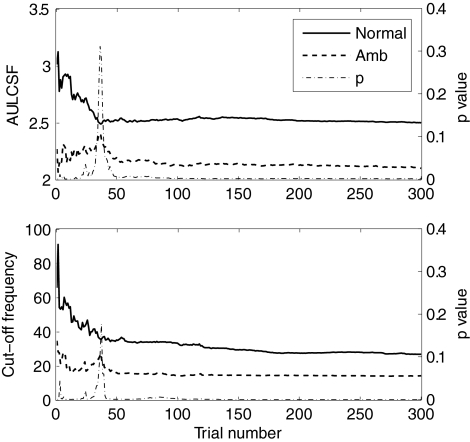
As a summary metric of the CSF function, the area under the CSF (AULCSF) is a broad measure of spatial vision,^{29,37,54–57} whereas the spatial frequency cutoff (cutSF) characterizes the high-frequency resolution of the visual system.^26,58 To characterize the contrast sensitivity differences between the normal and amblyopic participants, we calculated AULCSF and cutSF for each subject. The AULCSF was calculated as the integration from 0.5 cpd to the root of the log-parabola in the high-spatial-frequency range. The cutSF was defined as the spatial frequency at which contrast sensitivity is 2.0 (threshold = 0.5).

The average AULCSF and cutSF for both groups are shown as a function of trial number in Figure 8, along with running P-values from the t-test. The AULCSF differences between the groups became significant after approximately 40 trials (2.29 ± 0.36 vs. 2.53 ± 0.46, t₃₄ = −1.70, P < 0.05). After 39 trials, the cutoff frequency of the amblyopia group also became significantly lower than that of the normal group (19.4 ± 12.1 vs. 37.4 ± 26.5, t₃₄ = −2.51, P < 0.01). After 50 trials, the significance level of both differences remained high (P < 0.01).

Figure 8.

CSF differences between the normal and amblyopic groups. Top: AULCSF estimates for both groups as a function of trial number; bottom: cutSF estimates as a function of trial number. P-value is for the difference between the two groups.

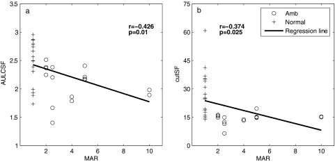
To explore the relationship between CSF features and visual acuity, we examined the correlations between AULCSF and cutSF with visual acuity. In the analysis, the averages of the final AULCSF and cutSF estimates from the two sessions were used, and the visual acuities of normal subjects were set at 1 minute. As showed in Figure 9, there was a negative correlation between the AULCSF and visual acuity (r = −0.426, P < 0.01). The correlation between the final cutSF and visual acuity was also significant (r = −0.374, P < 0.05). These analyses confirm a relationship between CSF metrics provided by the qCSF and visual acuity (the predominant clinical vision measure). The correlations are not significant if we restrict the analysis to the amblyopia group, perhaps due to the relatively small sample size. Although the CSF correlates with visual acuity, the two parameters may provide different measures of spatial vision.

Figure 9.

Correlations between visual acuity and CSF measures obtained with the qCSF. (a) The AULCSF and (b) the cutSF correlated negatively with visual acuity (in MAR).

Screening Amblyopia According to qCSF Features

The significant difference of the AULCSF and cutSF between the normal and amblyopia groups prompted us to evaluate them as potential measures for amblyopia screening. A logistic regression⁵⁹ analysis based on the AULCSF and cutSF was used to predict membership in the two groups

where P(amb) is the probability of a subject's having amblyopia, area represents AULCSF, sf represents cutSF, and βs are the coefficients.

We first estimated the coefficients based on the final AULCSFs and cutSFs of each observer, obtained by treating the final results from both qCSF sessions as independent datasets. The results are: β₀ = 7.41, β₁ = 5.85, and β₂ = −1.22 (Hosmer and Lemeshow goodness-of fit-test, χ²₇ = 5.00, P = 0.661). There was no significant difference between the predicted and the observed values.

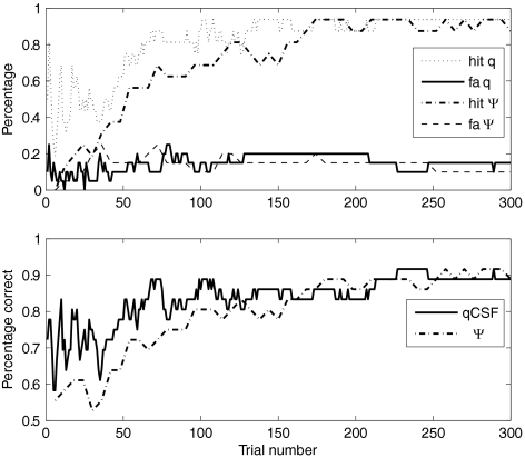
With these coefficients, we then calculated the probability of each subject's having amblyopia after each trial of qCSF. A subject with a P > 0.5 was categorized as an amblyope. The hit rate, false alarm rate, and percentage of correct classifications after each qCSF trial in the two sessions were averaged and plotted as functions of the number of trials (Fig. 10). The mean accuracy of the prediction was 77.8% after 50 trials with a low false alarm rate of 10%. The accuracy of the prediction was 88.9% in 300 trials. This result shows the potential of the qCSF method in screening amblyopia.

Figure 10.

The hit rate, false alarm (fa) rate, and percentage correct of the logistic regression model in predicting the probability of amblyopia as a function of trials based on both the qCSF and Ψ methods.

We conducted similar analyses on the CSF estimates obtained from the Ψ method. A log-truncated parabolic model was fitted to the Ψ CSF (thresholds at six spatial frequencies) to get estimates of four CSF parameters (γ_max, ƒ_max, β, and δ). AULCSF and cutSF were calculated from the best-fitting parameters. Noting that the Ψ CSF data were composed by thresholds at six spatial frequencies, each prediction of the running analysis was based on multiples of six trials. The hit, false alarm, and percentage correct as functions of trials are plotted in Figure 10. The accuracy of the Ψ prediction was 72.2% in 54 trials. The accuracy of the Ψ method was lower than that of qCSF until ∼170 trials. After 180 trials, the predictions from both methods are almost the same. The percentage correct of final prediction by the Ψ method is 88.9%, the same as the prediction of the qCSF with 300 trials.

Discussion

In this study, we compared the CSFs of 10 normal subjects and 8 amblyopes measured by the qCSF³⁷ and Ψ³⁶ methods. The precision, accuracy, and test–retest reliability of the qCSF method were evaluated. Our analysis validated the assumptions of the qCSF method in observers with normal and amblyopic vision. The method's CSF model (truncated log-parabola) can well describe individual CSF data, and the psychometric slope is constant across different spatial frequencies for most subjects. Moreover, additional analyses showed that approximately 50 qCSF trials could capture the differences in CSF features (AULCSF and cutSF) between the normal and amblyopia groups. By adopting a logistic regression, we demonstrated the potential of qCSF for screening amblyopia with an accuracy of 77.8% in 50 trials. Taken together, our results demonstrate the potential of the qCSF method, an accurate and precise method of measuring CSFs in both normal people and amblyopes, as a tool for clinical practice.

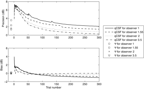
To simplify the CSF model used in the qCSF, we fixed the psychometric slope at 3.5 across spatial frequencies based on the QUEST method's slope assumptions.³⁵ However, the mean estimated value of slopes (1.55 ± 0.47) for all participants was much less than 3.5. To examine the effects of this parameter mismatch on our results, we simulated CSF measurements on an observer whose underlying psychometric functions have a slope of 1.55, with both the qCSF and Ψ methods that assume four different predefined slopes (1, 1.55, 2, and 3.5). The simulation had 500 iterations, each of which consisted of 300 qCSF trials and 50 × 6 Ψ trials.

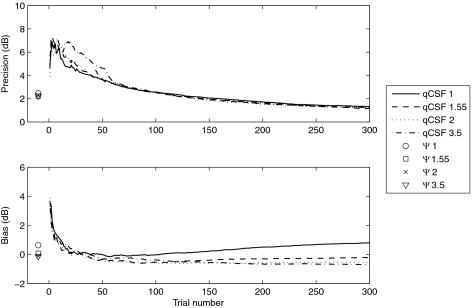
The precision of both methods is plotted as a function of trial number in the top panel of Figure 11. The precision of the CSFs obtained with the Ψ method was 2.45, 2.21, 2.24, and 2.34 dB for the predefined slopes 1, 1.55, 2.5, and 3.5, respectively. The four precision curves generated by the qCSF method with the four different predefined slopes overlapped almost completely. This result suggests that the predefined slope value did not affect the precision of measurement of either method. In fact, the observed precision of the qCSF method for normal observers after 100 trials was 2.63 dB, with a predefined slope of 3.5. The precision is well matched to the result for normal subjects (2.79 dB), with a predefined slope of 2 reported by Lesmes et al.³⁷

Figure 11.

The CSF of a simulated observer with psychometric slope of 1.55 was measured by both the qCSF and Ψ methods, with four different predefined slopes (1, 1.55, 2.5, and 3.5). Single symbols represent the results from the Ψ method.

The bias of the threshold estimates of both methods is plotted as a function of trial number in the bottom panel of Figure 11. The mean bias for the CSFs estimated using the Ψ method was 0.63, 0.09, −0.12 and −0.06 dB for predefined slopes 1, 1.55, 2.5, and 3.5, respectively. For the qCSF method, a predefined slope of 1, smaller than the actual value, led to threshold overestimates and a predefined slope larger than actual value caused threshold underestimates. The final bias of the qCSF method for a predefined slopes of 1, 1.55, 2.5, and 3.5 was 0.80, −0.21, −0.69, and −0.75 dB, respectively. The difference in bias between predefined slopes of 1.55 and 3.5 was −0.54 dB. Given the almost 2.5-fold difference in slope values between the underlying psychometric functions, this difference is very small (∼6%). The simulation results suggest minimal effects of slope parameter mismatch on the conclusions of the current experiment, and that the qCSF and Ψ methods may work well without the very precise knowledge of the true slope. These results suggest that an assumed slope of 2.0 may be ideal for future qCSF applications.

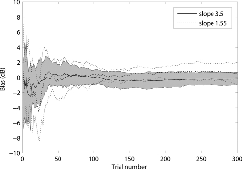
To further investigate the effects of parameter mismatch, we obtained an additional data set from another six normal subjects using both the Ψ and qCSF methods with a predefined slope of 1.55. The average bias of these six subjects from the original measurements with a predefined slope of 3.5 and the new measurements are plotted in Figure 12. There was no significant difference between biases under the two slope settings for 98.3% of the trials (P > 0.10; t-test). For 94% of the trials, the bias with slope 1.55 did not differ from 0 (for these trials, P > 0.1; t-test). Taken together with the results of the previous analysis, we conclude that the steep slope value predefined in the qCSF program did not appreciably affect our results.

Figure 12.

The bias curves for the 3.5 and 1.55 slopes. Shaded region represents 1 SD for the 3.5 slope. The thin dotted lines indicate the variability of 1 SD for the 1.55 slope.

To further explore the flexibility of the qCSF method, we simulated CSF measurements on observers whose underlying psychometric functions have different slopes, 1, 1.55, 2.5, and 3.5, with both the qCSF and Ψ methods that assumed predefined slopes, 1, 1.55, 2.5, and 3.5 (a 4 × 4 design). The simulation had 500 iterations, each of which consisted of 300 qCSF trials and 50 × 6 Ψ trials. The precision and bias of the qCSF and Ψ methods under these 4 × 4 conditions are listed in Appendix B (see Tables A1 and A2). The results measured with predefined slope 3.5 are plotted in Figure 13. The final (300 trials) precision of the qCSF method, which used a model slope of 3.5, was 2.10, 1.45, 0.84, and 0.26 dB for observer slopes 1, 1.55, 2.5, and 3.5, respectively. The final bias was −1.02, −0.79, −0.29, and 0.01 dB for observer slopes 1, 1.55, 2.5, and 3.5, respectively. The precision and bias were proportional to the deviation between the slope of the observer's psychometric function and the predefined slope. Even in the worst situation, in which the predefined slope 3.5 deviated well away from the slope of the observer's psychometric function (1.0), the precision and bias were only 2.10 and −1.02 dB, respectively.

Figure 13.

The CSF of simulated observers with psychometric slopes of 1, 1.55, 2.5, and 3.5 was measured by both the qCSF and Ψ methods, with a predefined slope of 3.5. Single symbols represent the results from the Ψ method.

In test–retest analysis, the linear regression slope in the amblyopia group was closer to 1 than that in the normal group. It seemed that both methods were more reliable in the amblyopia group than in the normal group. However, it is worth noting that the normal participants had no previous experience in psychophysical experiments, and so, the slight loss of reliability in the normal group may be due to the learning effect across measurement sessions. To some extent, this finding is similar to that obtained in two other studies reported by Levi and Polat.^60,61 In these experiments, novices improved substantially after training, but participants who were highly practiced did not. This phenomenon raises another important question: how to minimize effects of practice during measurement. There is plenty of evidence that even a single testing session can introduce learning effects,⁶² and overexposure to certain tasks could lead to performance decrements.^63,64 With these considerations, the fewer trials a measurement takes, the less effect it may have on the results. On the other hand, a sufficient number of trials are necessary to achieve the desirable precision. The qCSF method may be one of the solutions to this dilemma in CSF measurement.

In the present study, we used a logistic model to classify amblyopia. The result showed that the CSFs obtained in 50 qCSF trials classified amblyopia with a reasonably high accuracy. One issue that naturally limits the use of the qCSF screening procedure is that the spatial vision deficit in amblyopia is not limited to deficient CSF.⁸ There are also critical problems of binocular combination that underlie the disorder.⁶⁵ Combining the results of qCSF with other binocular metrics may improve the diagnosis of amblyopia.

The qCSF method belongs to a new generation of adaptive methods that directly estimate increasingly elaborate psychophysical functions, including multidimensional models describing psychometric functions,^66,67 equidetectable elliptical contours in color space,⁴⁵ threshold versus external noise contrast (TvC) functions,⁶⁸ the spatiotemporal contrast sensitivity surface,⁶⁹ neural input–output relationships,^70–72 and the discrimination of memory-retention models.^73,74 These methods provide a powerful testing approach that is potentially important for many clinical applications. The present study provides a sample application.

Conclusion

The qCSF method, which applies an information-gain testing strategy that greatly reduces CSF testing time, demonstrates potential for laboratory research and clinical evaluation. To complement the validation by Lesmes et al.,³⁷ we validated the method for larger groups of observers with normal and abnormal vision. With 50 to 100 qCSF trials, which require only 2 to 6 minutes to complete, the CSF of a patient could be measured with acceptable precision and classified with logistic regression. We believe that with improvements in computing power and more powerful statistical tools, the qCSF method will be appropriate for use in screening amblyopia and other visual impairments.

Appendix A

Before measurement started, a prior probability distribution p₀(ν→), representing our knowledge about the tested CSF, was constructed with hyperbolic secants.⁷⁵ A conditional probability lookup table p(correct|x→,ν→) was initialized by calculating all the probabilities of correct response for all possible stimulus conditions T_x→ and all possible parameters T_ν→. As prescribed by Kontsevich and Tyler,³⁶ before the t+1th trial began, the qCSF program calculated:

1. The probability of a correct response in a given stimulus condition x̄

   
2. The posterior probability distribution p_t+1(ν→) after a correct and an incorrect response to each possible stimulus x→ in trial t+1

   

   
3. The entropies of the estimated posterior probability p_t+1(ν→) after a correct and an incorrect response to each possible stimulus x→

   

   
4. The expected entropy after a trial with stimulus x→

   
5. The stimulus providing the lowest expected entropy

   

   After the participants finished trial t+1 with stimulus condition x→_t+1, the qCSF program calculated:

6. The posterior probability distribution p_t+1(ν→|x→, correct) or p_t+1(ν→|x→, incorrect) was updated as p_t+1(ν→): p_t+1(ν→)=p_t+1(ν→|x→, correct) or p_t+1(ν→|x→, incorrect).

7. The expected value of ν→ was calculated

   

   After 300 trials were run, the program was terminated.

Appendix B

Parameter Mismatch

We simulated CSF measurements on observers whose underlying psychometric functions have slopes of 1, 1.55, 2.5, and 3.5, with both the qCSF and Ψ methods that assumed predefined slopes of 1, 1.55, 2.5, and 3.5. The simulation had 500 iterations, each of which consisted of 300 qCSF trials and 50 × 6 Ψ trials. The precision and bias were calculated. The precision and bias estimated in 50, 100, and 300 trials are shown in Tables A1 and A2 (unit: dB).

Table A1.

The Final Precision and Bias of the Ψ Method

	Precision (dB)				Bias (dB)
	OS 1	OS 1.55	OS 2.5	OS 3.5	OS 1	OS 1.55	OS 2.5	OS 3.5
MS 1	3.19	2.45	2.04	1.90	0.04	0.63	1.23	1.44
MS 1.55	3.10	2.21	1.77	1.61	−0.35	0.09	0.44	0.63
MS 2.5	3.27	2.24	1.65	1.48	−0.14	−0.12	0.02	0.18
MS 3.5	3.56	2.34	1.67	1.37	0.26	−0.06	−0.01	0.04

OS and MS are short for observer slope and model slope separately.

Table A2.

The Precision and Bias of the qCSF Method

	Precision (dB)				Bias (dB)
	OS 1	OS 1.55	OS 2.5	OS 3.5	OS 1	OS 1.55	OS 2.5	OS 3.5
50 Trials
MS 1	4.10	3.62	3.02	3.15	−0.28	−0.03	0.26	0.09
MS 1.55	4.20	3.70	3.42	3.85	−0.24	−0.36	−0.37	−0.41
MS 2.5	4.61	4.63	3.03	2.89	−0.08	−0.31	−0.45	−0.29
MS 3.5	4.85	4.01	3.15	2.62	0.13	0.16	0.00	−0.20
100 Trials
MS 1	3.06	2.57	2.16	2.05	−0.78	−0.01	0.58	0.69
MS 1.55	3.16	2.54	2.07	1.79	−0.70	−0.53	−0.10	0.12
MS 2.5	3.35	2.57	1.86	1.52	−0.50	−0.37	−0.30	−0.09
MS 3.5	3.44	2.79	1.89	1.46	−0.44	−0.29	−0.29	−0.14
300 Trials
MS 1	1.83	1.32	1.01	0.96	−0.41	0.80	1.67	2.06
MS 1.55	1.73	1.14	0.91	0.75	−1.07	−0.21	0.62	1.18
MS 2.5	1.99	1.24	0.56	0.30	−1.14	−0.69	−0.08	0.02
MS 3.5	2.10	1.41	0.84	0.26	−1.02	−0.75	−0.29	0.01

OS, observer slope; MS, model slope.

References

- 1. Ciuffreda KJ, Levi DM, Selenow A. Amblyopia: Basic and Clinical Aspects: London: Butterworth-Heinemann; 1991:10–14 [Google Scholar]
- 2. Levi DM, Li RW. Perceptual learning as a potential treatment for amblyopia: a mini-review. Vision Res. 2009;49:2535–2539 [DOI] [PMC free article] [PubMed] [Google Scholar]
- 3. Hess RF, Thompson B, Gole G, Mullen KT. Deficient responses from the lateral geniculate nucleus in humans with amblyopia. Eur J Neurosci. 2009;29:1064–1070 [DOI] [PMC free article] [PubMed] [Google Scholar]
- 4. Wu C, Hunter DG. Amblyopia: diagnostic and therapeutic options. Am J Ophthalmol. 2006;141:175–184 [DOI] [PubMed] [Google Scholar]
- 5. Niu J-l. Normallization of therapy is the key point to improve the effect of treatment for amblyopia. Chin J Ophthalmol. 2003;39:4 [Google Scholar]
- 6. Beauchamp CL, Felius J, Beauchamp GR, Brown MM, Brown GC. The economic value added for care of amblyopia, strabismus, and asthma. J AAPOS. 2007;11:76 [Google Scholar]
- 7. Ciuffreda KJ, Levi DM, Selenow A. Amblyopia: Basic and Clinical Aspects. London: Butterworth-Heinemann; 1991:78–93 [Google Scholar]
- 8. McKee SP, Levi DM, Movshon JA. The pattern of visual deficits in amblyopia. J Vis. 2003;3:380–405 [DOI] [PubMed] [Google Scholar]
- 9. Hess RF, McIlhagga W, Field DJ. Contour integration in strabismic amblyopia: the sufficiency of an explanation based on positional uncertainty. Vision Res. 1997;37:3145–3161 [DOI] [PubMed] [Google Scholar]
- 10. Hess RF, Demanins R. Contour integration in anisometropic amblyopia. Vision Res. 1998;38:889–894 [DOI] [PubMed] [Google Scholar]
- 11. Kozma P, Kiorpes L. Contour integration in amblyopic monkeys. Vis Neurosci. 2003;20:577–588 [DOI] [PubMed] [Google Scholar]
- 12. Simmers AJ, Ledgeway T, Hess RF, McGraw PV. Deficits to global motion processing in human amblyopia. Vision Res. 2003;43:729–738 [DOI] [PubMed] [Google Scholar]
- 13. Simmers AJ, Ledgeway T, Hess RF. The influences of visibility and anomalous integration processes on the perception of global spatial form versus motion in human amblyopia. Vision Res. 2005;45:449–460 [DOI] [PubMed] [Google Scholar]
- 14. Della Sala S, Bertoni G, Somazzi L, Stubbe F, Wilkins AJ. Impaired contrast sensitivity in diabetic patients with and without retinopathy: a new technique for rapid assessment. Br J Ophthalmol. 1985;69:136–142 [DOI] [PMC free article] [PubMed] [Google Scholar]
- 15. Hess RF. Contrast sensitivity assessment of functional amblyopia in humans. Trans Ophthalmol Soc UK. 1979;99:391–397 [PubMed] [Google Scholar]
- 16. Hess RF, Howell ER. The threshold contrast sensitivity function in strabismic amblyopia: evidence for a two type classification. Vision Res. 1977;17:1049–1055 [DOI] [PubMed] [Google Scholar]
- 17. Jindra LF, Zemon V. Contrast sensitivity testing: a more complete assessment of vision. J Cataract Refract Surg. 1989;15:141–148 [DOI] [PubMed] [Google Scholar]
- 18. Marmor MF. Contrast sensitivity and retinal disease. Ann Ophthalmol. 1981;13:1069–1071 [PubMed] [Google Scholar]
- 19. Marmor MF. Contrast sensitivity versus visual acuity in retinal disease. Br J Ophthalmol. 1986;70:553–559 [DOI] [PMC free article] [PubMed] [Google Scholar]
- 20. Marmor MF, Gawande A. Effect of visual blur on contrast sensitivity: clinical implications. Ophthalmology. 1988;95:139–143 [DOI] [PubMed] [Google Scholar]
- 21. Montes-Mico R, Ferrer-Blasco T. Contrast sensitivity function in children: normalized notation for the assessment and diagnosis of diseases. Doc Ophthalmol. 2001;103:175–186 [DOI] [PubMed] [Google Scholar]
- 22. Onal S, Yenice O, Cakir S, Temel A. FACT contrast sensitivity as a diagnostic tool in glaucoma: FACT contrast sensitivity in glaucoma. Int Ophthalmol. 2008;28:407–412 [DOI] [PubMed] [Google Scholar]
- 23. Wolkstein M, Atkin A, Bodis-Wollner I. Contrast sensitivity in retinal disease. Ophthalmology. 1980;87:1140–1149 [DOI] [PubMed] [Google Scholar]
- 24. Woo GC, Dalziel CC. A pilot study of contrast sensitivity assessment of the CAM treatment of amblyopia. Acta Ophthalmol. 1981;59:35–37 [DOI] [PubMed] [Google Scholar]
- 25. Yenice O, Onal S, Incili B, Temel A, Afsar N, Tanridag T. Assessment of spatial-contrast function and short-wavelength sensitivity deficits in patients with migraine. Eye. 2007;21:218–223 [DOI] [PubMed] [Google Scholar]
- 26. Huang C, Tao L, Zhou Y, Lu ZL. Treated amblyopes remain deficient in spatial vision: a contrast sensitivity and external noise study. Vision Res. 2007;47:22–34 [DOI] [PubMed] [Google Scholar]
- 27. Pelli DG, Robson JG, Wilkins AJ. The design of a new letter chart for measuring contrast sensitivity. Clin Vision Sci. 1988;2:187–199 [Google Scholar]
- 28. Regan D, Giaschi DE, Fresco BB. Measurement of glare susceptibility using low-contrast letter charts. Optom Vis Sci. 1993;70:969–975 [DOI] [PubMed] [Google Scholar]
- 29. van Gaalen KW, Jansonius NM, Koopmans SA, Terwee T, Kooijman AC. Relationship between contrast sensitivity and spherical aberration: comparison of 7 contrast sensitivity tests with natural and artificial pupils in healthy eyes. J Cataract Refract Surg. 2009;35:47–56 [DOI] [PubMed] [Google Scholar]
- 30. Pesudovs K, Hazel CA, Doran RM, Elliott DB. The usefulness of Vistech and FACT contrast sensitivity charts for cataract and refractive surgery outcomes research. Br J Ophthalmol. 2004;88:11–16 [DOI] [PMC free article] [PubMed] [Google Scholar]
- 31. Hohberger B, Laemmer R, Adler W, Juenemann AG, Horn FK. Measuring contrast sensitivity in normal subjects with OPTEC 6500: influence of age and glare. Graefes Arch Clin Exp Ophthalmol. 2007;245:1805–1814 [DOI] [PubMed] [Google Scholar]
- 32. Buhren J, Terzi E, Bach M, Wesemann W, Kohnen T. Measuring contrast sensitivity under different lighting conditions: comparison of three tests. Optom Vis Sci. 2006;83:290–298 [DOI] [PubMed] [Google Scholar]
- 33. Bradley A, Hook J, Haeseker J. A comparison of clinical acuity and contrast sensitivity charts: effect of uncorrected myopia. Ophthalmic Physiol Opt. 1991;11:218–226 [PubMed] [Google Scholar]
- 34. Ginsburg AP. Contrast sensitivity and functional vision. Int Ophthalmol Clin. 2003;43:5–15 [DOI] [PubMed] [Google Scholar]
- 35. Watson AB, Pelli DG. QUEST: a Bayesian adaptive psychometric method. Percept Psychophys. 1983;33:113–120 [DOI] [PubMed] [Google Scholar]
- 36. Kontsevich LL, Tyler CW. Bayesian adaptive estimation of psychometric slope and threshold. Vision Res. 1999;39:2729–2737 [DOI] [PubMed] [Google Scholar]
- 37. Lesmes LA, Lu Z-L, Baek J, Albright T. Efficient Adaptive Estimation of the Contrast Sensitivity Function: the qCSF method. J Vis. [DOI] [PMC free article] [PubMed] [Google Scholar]
- 38. Cobo-Lewis AB. An Adaptive Method for Estimating Multiple Parameters of a Psychometric Function. Presented at the 29th Annual Meeting of the Society for Mathematical Psychology Chapel Hill, NC: University of North Carolina,; 1996 [Google Scholar]
- 39. Watson AB, Ahumada AJ., Jr A standard model for foveal detection of spatial contrast. J Vis. 2005;5:717–740 [DOI] [PubMed] [Google Scholar]
- 40. Rohaly AM, Owsley C. Modeling the contrast-sensitivity functions of older adults. J Opt Soc Am. 1993;10:1591–1599 [DOI] [PubMed] [Google Scholar]
- 41. Wichmann FA, Hill NJ. The psychometric function: I. Fitting, sampling, and goodness of fit. Percept Psychophys. 2001;63:1293–1313 [DOI] [PubMed] [Google Scholar]
- 42. Swanson WH, Birch EE. Extracting thresholds from noisy psychophysical data. Percept Psychophys. 1992;51:409–422 [DOI] [PubMed] [Google Scholar]
- 43. Green DM. Maximum-likelihood procedures and the inattentive observer. J Acoust Soc Am. 1995;97:3749–3760 [DOI] [PubMed] [Google Scholar]
- 44. Cobo-Lewis AB. An adaptive psychophysical method for subject classification. Percept Psychophys. 1997;59:989–1003 [DOI] [PubMed] [Google Scholar]
- 45. Kujala JV, Lukka TJ. Bayesian adaptive estimation: the next dimension. J Math Psychol. 2006;50:369–389 [Google Scholar]
- 46. Strasburger H. Invariance of the psychometric function for character recognition across the visual field. Percept Psychophys. 2001;63:1356–1376 [DOI] [PubMed] [Google Scholar]
- 47. Li X, Lu ZL, Xu P, Jin J, Zhou Y. Generating high gray-level resolution monochrome displays with conventional computer graphics cards and color monitors. J Neurosci Methods. 2003;130:9–18 [DOI] [PubMed] [Google Scholar]
- 48. Brainard DH. The Psychophysics Toolbox. Spat Vis. 1997;10:433–436 [PubMed] [Google Scholar]
- 49. Pelli DG. The VideoToolbox software for visual psychophysics: transforming numbers into movies. Spat Vis. 1997;10:437–442 [PubMed] [Google Scholar]
- 50. Wichmann FA, Hill NJ. The psychometric function: II. Bootstrap-based confidence intervals and sampling. Percept Psychophys. 2001;63:1314–1329 [DOI] [PubMed] [Google Scholar]
- 51. Strasburger H. Converting between measures of slope of the psychometric function. Percept Psychophys. 2001;63:1348–1355 [DOI] [PubMed] [Google Scholar]
- 52. Watson AB. Probability summation over time. Vision Res. 1979;19:515–522 [DOI] [PubMed] [Google Scholar]
- 53. Lu ZL, Lesmes LA, Dosher BA. Spatial attention excludes external noise at the target location. J Vis. 2002;2:312–323 [DOI] [PubMed] [Google Scholar]
- 54. Oshika T, Okamoto C, Samejima T, Tokunaga T, Miyata K. Contrast sensitivity function and ocular higher-order wavefront aberrations in normal human eyes. Ophthalmology. 2006;113:1807–1812 [DOI] [PubMed] [Google Scholar]
- 55. Oshika T, Klyce SD, Applegate RA, Howland HC. Changes in corneal wavefront aberrations with aging. Invest Ophthalmol Vis Sci. 1999;40:1351–1355 [PubMed] [Google Scholar]
- 56. Applegate RA, Howland HC, Sharp RP, Cottingham AJ, Yee RW. Corneal aberrations and visual performance after radial keratotomy. J Refract Surg. 1998;14:397–407 [DOI] [PubMed] [Google Scholar]
- 57. Applegate RA, Hilmantel G, Howland HC, Tu EY, Starck T, Zayac EJ. Corneal first surface optical aberrations and visual performance. J Refract Surg. 2000;16:507–514 [DOI] [PubMed] [Google Scholar]
- 58. Zhou Y, Huang C, Xu P, et al. Perceptual learning improves contrast sensitivity and visual acuity in adults with anisometropic amblyopia. Vision Res. 2006;46:739–750 [DOI] [PubMed] [Google Scholar]
- 59. Hosmer DW, Lemeshow S. Applied Logistic Regression. New York: Wiley; 1989 [Google Scholar]
- 60. Levi DM, Polat U. Neural plasticity in adults with amblyopia. Proc Natl Academy Sci U S A. 1996;93:6830–6834 [DOI] [PMC free article] [PubMed] [Google Scholar]
- 61. Levi DM, Polat U, Hu YS. Improvement in Vernier acuity in adults with amblyopia: practice makes better. Invest Ophthalmol Vis Sci. 1997;38:1493–1510 [PubMed] [Google Scholar]
- 62. Fine I, Jacobs RA. Comparing perceptual learning tasks: a review. J Vis. 2002;2:190–203 [DOI] [PubMed] [Google Scholar]
- 63. Censor N, Karni A, Sagi D. A link between perceptual learning, adaptation and sleep. Vision Res. 2006;46:4071–4074 [DOI] [PubMed] [Google Scholar]
- 64. Ofen N, Moran A, Sagi D. Effects of trial repetition in texture discrimination. Vision Res. 2007;47:1094–1102 [DOI] [PubMed] [Google Scholar]
- 65. Huang C-B, Zhou J, Lu Z-L, Feng L, Zhou Y. Binocular combination in anisometropic amblyopia. J Vis. 2009;9:1–16 [DOI] [PMC free article] [PubMed] [Google Scholar]
- 66. Tanner T, Hill N, Rasmussen C, Wichmann F. Efficient adaptive sampling of the psychometric function by maximizing information gain. Proceedings of the 8th Tübingen Perception Conference; Tubingen, Germany 2005 [Google Scholar]
- 67. Remus JJ, Collins LM. A comparison of adaptive psychometric procedure based on the theory of optimal experiments and Bayesian techniques: implications for cochlear implant testing. Percept Psychophys. 2007;69:311–323 [DOI] [PubMed] [Google Scholar]
- 68. Lesmes LA, Jeon ST, Lu ZL, Dosher BA. Bayesian adaptive estimation of threshold versus contrast external noise functions: the quick TvC method. Vision Research. 2006;46:3160–3176 [DOI] [PubMed] [Google Scholar]
- 69. Lesmes LA, Gepshtein S, Lu Z-L, Albright T. Rapid estimation of the spatiotemporal contrast sensitivity surface. J Vis. 2009;9:696 [Google Scholar]
- 70. Lewi J, Butera R, Paninski L. Real-time adaptive information-theoretic optimization of neurophysiology experiments. Adv Neural Inform Process Syst. 2007;19:857 [Google Scholar]
- 71. Lewi J, Butera R, Paninski L. Sequential optimal design of neurophysiology experiments. Neural Comput. 2009;21:619–687 [DOI] [PubMed] [Google Scholar]
- 72. Paninski L. Asymptotic theory of information-theoretic experimental design. Neural Comput. 2005;17:1480–1507 [DOI] [PubMed] [Google Scholar]
- 73. Myung J, Pitt M. Optimal experimental design for model discrimination. Psychol Rev. 2009;116:48–518 [DOI] [PMC free article] [PubMed] [Google Scholar]
- 74. Cavagnaro DR, Myung JI, Pitt MA, Kujala JV. Adaptive design optimization: a mutual information based approach to model discrimination in cognitive science. Neural Comput. 2010;22:887–905 [DOI] [PubMed] [Google Scholar]
- 75. King-Smith PE, Rose D. Principles of an adaptive method for measuring the slope of the psychometric function. Vision Res. 1997;37:1595–1604 [DOI] [PubMed] [Google Scholar]