Test-Retest Reliability of Arterial Spin Labeling with Common Labeling Strategies

Abstract

Purpose

To compare the test-retest reproducibility of pseudo-continuous arterial spin labeling (ASL) with pulsed (PASL) and continuous (CASL) ASL.

Materials and methods

Twelve healthy subjects were scanned on a 3.0T scanner with PASL, CASL and pCASL. Scans were repeated within-session, after 1 hour and after 1 week to assess reproducibility at different scan intervals.

Results

Comparison of within-subject coefficients of variation (wsCV) demonstrated high within-session reproducibility (i.e. low wsCV) for CASL-based methods (gray matter (GM) wsCV for pCASL: 3.5% ± 0.02%, CASL: 4.1% ± 0.07%) compared to PASL (wsCV: 7.5% ± 0.06%), due to the higher signal-to-noise ratio (SNR) associated with continuous labeling, evident in the 20% gain in temporal SNR and 58% gain in raw SNR for pCASL relative to PASL. At the one week scan interval, comparable reproducibility between PASL (GM wsCV 9.2% ± 0.12%) and pCASL (GM wsCV 8.5% ± 0.14%) was observed, indicating the dominance of physiological fluctuations.

Conclusion

Although all three approaches are capable of measuring cerebral blood flow within a few minutes of scanning, the high precision and SNR of pCASL, with its insensitivity to vessel geometry, make it an appealing method for future ASL application studies.

INTRODUCTION

Arterial spin labeling (ASL) is a MRI-based method that utilizes blood as an endogenous tracer through altering its magnetization with radiofrequency (RF) field and provides noninvasive quantification of tissue perfusion based on images acquired with ASL or control labeling. ASL can be considered as a form of magnetization preparation that can be combined with almost any imaging sequence, though sequences with high signal-to-noise ratio (SNR) that are resistant to motion degradation are preferred. Two major categories of ASL are in common use: pulsed (PASL) and continuous (CASL). PASL methods use a short (~10ms) RF pulse to instantaneously invert blood spins in a thick slab while CASL uses either continuous wave RF or a long train of pulses (~2s) to invert blood spins flowing through a labeling plane based on the principles of adiabatic fast passage (AFP) (1).

PASL methods have been the most widely used methods to date because of their ease of implementation and low specific absorption rate (SAR), even though their sensitivity is theoretically a factor of e (~2.72) lower than CASL (2). In practice, it has been difficult to achieve the full sensitivity of CASL for multislice imaging implementations due to inefficiencies in control labeling schemes (3). Furthermore, successful labeling of blood spins with CASL depends on whether the adiabatic condition is satisfied, which is highly dependent on flow velocity component that is perpendicular to the labeling plane (4), making CASL sensitive to vascular geometry. Studies have shown PASL has high labeling efficiency (~0.97) that is relatively stable for a wide range of flow velocities (2), which implies PASL may have better reproducibility than the more complicated CASL. Meanwhile, the migration from unitary transmit and receive RF coils to body transmit and array receiver systems has increased the appeal of PASL by allowing larger labeling slabs while providing greater challenges for CASL from the perspective of SAR deposition.

Recently, pseudo-CASL (pCASL) was introduced (5–6). pCASL uses a train of discrete RF pulses to achieve labeling of flowing blood spins in a manner similar to CASL, however “adiabatic inversion” or labeling in pCASL is predominantly achieved through phase shifts caused by the mean gradients applied between RF pulses and is less dependent on flow velocity than CASL, making pCASL potentially somewhat less sensitive to variations in flow velocity and vascular geometry than CASL. The train of short duration RF pulses used in pCASL is also less demanding in terms of RF duty cycle, therefore pCASL can take full advantage of the array coil and body transmission combination. Moreover, pCASL can be implemented with higher labeling efficiency than CASL (~85%) due to better control of magnetization transfer effects. These advantages suggest that pCASL may outperform the existing ASL methods in terms of SNR and precision in CBF measurement.

To determine the relative performance of these methods, we assessed the reproducibility of PASL, CASL and pCASL acquired on a 3T scanner in healthy subjects. Since all images were acquired using the same gradient-echo echoplanar imaging (GE-EPI) method and similar transit delays were used, this study is essentially a comparison between three different labeling strategies. Both system-related errors and physiological fluctuations were investigated by assessing the reproducibility of cerebral blood flow (CBF) measurements performed within-session, as well as after 1 hour and 1 week. Similar single-blood-compartment models based on modification of the Bloch equation for T₁ relaxation to include perfusion effects were used to quantify CBF for all three methods (7–8), using literature values for other parameters such as labeling efficiency, T₁ of blood and brain, and the blood:brain partition coefficient for water.

METHODS

Subjects

A total of 12 healthy subjects were recruited (7 females, 5 males, mean age 24±5) in accordance with the university’s institutional review board and informed consent was obtained from all subjects prior to scanning. To minimize modulations of blood flow, subjects were requested to abstain from caffeine for 12 hours prior to scanning. The majority of scans were performed between 8am and 11am to minimize diurnal fluctuations in blood flow (9). Three subjects were scanned between 3pm–6pm due to scheduling difficulties; however, their repeat scans were scheduled at the same time of the day to minimize time-of-day effects. Test-retest reproducibility was assessed for within-session, after one hour, and after one week. Subjects were removed from the scanner and repositioned for the one hour and one week scans. To ensure minimal change in subject position between the scan sessions, subjects were positioned such that their shoulders were touching the end of the head coils. Rotation was minimized by aligning subjects with the central beam of the head coils. All scans were performed during unconstrained rest, with subjects remaining awake inside the scanner.

MR Imaging

Data were collected on a 3T Siemens Trio whole-body scanner (Erlangen, Germany) equipped with both an eight-channel receive-only head coil (InVivo, USA) and a circularly-polarized transmit-receive (Tx/Rx) head coil (Bruker, Germany). Sequence parameters for the three pulse sequences tested are listed as follows:

For PASL, flow-sensitive alternating inversion recovery (FAIR) (10) with QUIPSS II (11) was implemented, which applies multiple saturation pulses proximal to the imaging region at TI₁ after global or slice-selective inversion to create a well-defined bolus of tagged blood. For the control scan, a hyperbolic-secant pulse (15.36ms, bandwidth 3.4kHz, 22.5μT) was applied to a slab covering the imaging region with additional 1cm gap on either side to account for slice profile imperfections. Instead of the standard nonselective inversion acquisition used in the original FAIR implementation, the label scan of the current study used an extended inversion slab covering an additional 10cm on either side of control inversion slab. This modification was necessary for body coil transmission because the traditional global inversion would result in unnecessary tagging that could contaminate the ASL signal in subsequent repetitions (12). Other ASL parameters include TI₁/TI₂ of 700ms/1700ms, which were based on previously published estimates of the temporal width for a 10cm tag bolus in healthy subjects (11).

For pCASL, the balanced labeling method (6) was implemented with mean G_z of 0.6mT/m and 1640 Hanning window shaped pulses for a total labeling duration of 1.5s (RF duration 500us with 360us gap in between, 5.2μT). Labeling was performed at 80mm below the center of imaging region, and a post-labeling delay of 1s was inserted to allow the label to enter the imaging slices. All pCASL data were acquired with the body coil transmission and head array-coil receiving combination, which allows a direct comparison between pCASL and PASL.

Amplitude-modulated (AM)-CASL (3,13) was performed with 2.25μT RF irradiation and 1.6 mT/m gradient at 80mm below the imaging region for a total labeling time of 2s, and post-labeling delay was set to 1s. Due to the high RF duty-cycle, CASL was limited to the Tx/Rx head coil. CASL data was only collected on a subset of 7 subjects (2 females, 5 males, mean age 25±6) due to technical difficulties with the Tx/Rx head coil.

All three sequences were acquired with GE-EPI at an in-plane resolution of 3.75 × 3.75 mm², 6mm slice thickness, 1mm slice gap, TE/TR=17ms/4s. 14 axial slices prescribed to cover the entire brain and collected in ascending order. To ensure the same coverage between sessions, the top of the imaging region always coincides with the top of the brain. 40 pairs of alternating control and tag images were acquired for each session of each sequence.

For PASL quantification, an additional M₀ scan was collected using the same GE-EPI sequence without the FAIR inversion pulses. High resolution (1mm³ isotropic resolution) anatomical images were also collected using MPRAGE (14) for image registration purposes.

Data Analysis

Magnitude images from the scanner were further analyzed using in-house developed scripts in Matlab (The Mathworks Inc., Natick, MA, USA). Unsubtracted magnitude images were first motion-corrected to the first image of the series via a six-parameter rigid body spatial transformation and co-registered to the corresponding MPRAGE images in SPM5 (http://www.fil.ion.ucl.ac.uk/spm/). Perfusion images were generated by pair-wise subtraction between the control and tag pairs and averaged over time. For PASL, the following equation (8) was used to convert the perfusion map to quantitative physiological units (ml/100g/min):

$$f=\frac{\lambda ·\mathrm{\Delta }M}{2\alpha ·M_0·{TI}_1·e^{-{TI}_2/T_{1b}}},$$

where λ is blood/tissue water partition coefficient (0.9g/ml), ΔM is the difference signal between control and label states, α is inversion efficiency assumed to be 0.95 (2), M₀ is equilibrium magnetization from the M₀ acquisition, TI₁/TI₂=700/1700ms and T_1b is T₁ of blood = 1664ms (15).

CASL and pCASL images were calibrated to physiological units using the single-blood-compartment model (7):

$$f=\frac{\lambda ·\mathrm{\Delta }M}{2\alpha ·M_0·T_{1b}·(e^{-w/T_{1b}}-e^{-(\tau +w)/T_{1b}})},$$

where α =0.85 for pCASL (5), 0.68 for AM-CASL (13), M₀ is the equilibrium magnetization of brain tissue, approximated by the mean of the control images, w is post labeling delay = 1s, and τ is labeling duration, set to 1.5s for pCASL and 2s for CASL.

All quantitative CBF maps were normalized to MNI space with SPM5. Standard anatomical regions-of-interest (ROIs) from WFU Pickatlas (Wake Forest University http://fmri.wfubmc.edu/cms/software) and major vascular territories based on previously published templates (16) were applied to the normalized images in SPM5 to extract the CBF values for comparison. Prior to reproducibility analysis, differences between measurements were tested for normality using the Shapiro-Wilk W test. Reproducibility was assessed by calculating the following quantities:

1. Intraclass Correlation Coefficient (ICC) (17)–relative measure of reliability which measures the contribution of between subject variances to total variance. ICC essentially measures the ability of a method to detect differences between subjects consistently, and typically ranges between 0–1. ICC values close to 1 indicate high reliability. For this study, two-way model, average-measures ICC were calculated using SPSS (SPSS Inc. v18.0, Chicago, IL).

2. within-subject coefficient of variation (wsCV) (18)—ratio of the standard deviation (SD) of the difference between repeated measurements to the mean of repeated measurements. This is typically reported as a percentage of the mean measured value. The smaller the wsCV, the smaller the SD is for the difference between measurements.

SNR differences between the three sequences were assessed by calculating both temporal and raw SNR for the mean perfusion images using whole brain masks. Temporal SNR (tSNR) was defined as mean signal of time series divided by the SD across time. Raw SNR (rSNR) was calculated as the ratio between mean signal and background noise. All SNR values were normalized to PASL for easy comparison.

To investigate the stability of the ASL signal as a function of number of averages (NA), 10 perfusion maps were calculated for each NA for every subject. NA ranged from 1 to 20. Whole brain GM mask derived from segmentation of MPRAGE images in SPM5 was used to obtain the mean GM CBF for each perfusion map generated. The coefficient of variation (CV) was calculated as 100*SD GM CBF/mean GM CBF from the 10 perfusion maps for each NA. The group mean (±SD) CVs were plotted against NA and a 1/√NA function was fitted to the data.

As an additional assessment of the ability of the three sequences in detecting differences between individuals, gender effects were compared by averaging data from all four sessions of each sequence.

RESULTS

Sample CBF maps in ml/100g/min calculated from 40 averages for the three sequences from 4 representative subjects are shown in Figure 1, where no major differences were detected in the CBF maps generated by the three sequences. Mean CBF estimates from CASL were consistently lower than CBF estimated from PASL and pCASL (repeated measures ANOVA: F_2,12=38.3, p<0.005).

Figure 1.

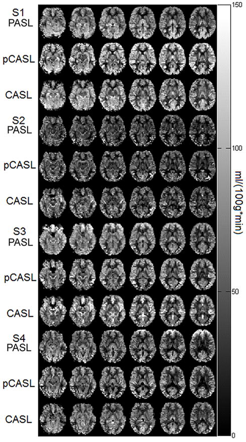
CBF maps (in units of ml/100g/min) spatially normalized to MNI space calculated from one session (40 averages) of each of the three sequences (from top to bottom: PASL, pCASL, CASL) for 4 representative subjects.

Plots of gray and white matter CBF values for scans repeated within-session, after 1 hour and after 1 week for all three sequences are shown in Figure 2 with the line of equality. As the scan interval increased, correlations became visibly poorer, likely dominated by physiological fluctuations (see Discussion). Of the three sequences, rescans for pCASL have the highest correlations in gray matter (GM). This was not observed in the white matter (WM) correlations, possibly due to the low SNR of WM for all three ASL sequences.

Figure 2.

Plots of GM (left) and WM (right) CBF values for the different scan intervals of the three sequences. Black line represents the line of equality.

A summary of the mean (±SD) CBF for all sessions of the different sequences, as well as the wsCV (and 95% confidence interval of wsCV estimate) of GM, WM and several commonly used ROIs are shown in Table 1. The same information for vascular territories, which included the left and right anterior (ACA), medial (MCA) and posterior (PCA) cerebral arteries, is shown in Table 2. ROIs where the differences between measurements were not normally distributed according to the Shapiro-Wilk W test are shown in boldface. Since log-normal transformation of a subtraction yields a ratio between the two measurements rather than absolute values, making it difficult for comparison between the ROIs, wsCVs reported here were calculated without log-normal transformation. While both CASL and pCASL had excellent within-session wsCV (less than 5%), wsCV for CASL became progressively worse for longer scan intervals. At the one week interval, PASL and pCASL had similar wsCVs. The wsCVs of other ROIs were noticeably worse than GM and WM values due to the smaller sizes of these regions, but in general pCASL and PASL have similar wsCVs at the one week interval. Interestingly, in the posterior cingulate and precuneus, wsCVs for CASL at 1hr was twice that of other ROIs (see Discussion).

Table 1.

Mean (SD) and wsCV (95% CI) of various ROIs for the three sequences. Abnormally distributed data are shown in boldface, but no log-normal transformation was attempted for better comparison of the wsCV estimates.

		PASL (N=12)				PCASL (N=12)				CASL (N=7)
		Scan1	Scan2	1 Hour	1 Week	Scan1	Scan2	1 Hour	1 Week	Scan1	Scan2	1 Hour	1 Week
GM	Mean±SD	61.9±6.6	61.9±5.7	61.1±7.0	59.8±8.7	60.5±8.5	60.3±7.1	62.2±6.4	60.4±9.9	44.5±10.7	45.2±9.9	39.3±5.6	50.7±8.9
	wsCV(%) 95%CI		7.5(0.06)	6.2(0.05)	9.2(0.12)		3.5(0.02)	5.5(0.05)	8.5(0.14)		4.1(0.07)	21.0(1.14)	16.6(0.74)
WM	Mean±SD	42.6±6.4	43.4±4.5	42.1±6.3	41.8±8.1	40.9±7.5	40.2±6.2	41.2±5.2	41.1±8.2	32.3±6.5	32.5±7.0	28.1±3.4	36.0±6.4
	wsCV(%) 95%CI		9.5(0.12)	8.0(0.11)	12.8(0.29)		8.0(0.15)	9.3(0.17)	12.0(0.36)		4.8(0.08)	18.4(0.69)	13.8(0.49)
Hippocampus	Mean±SD	63.4±9.6	67.5±8.0	61.1±9.4	61.5±11.4	57.3±10.3	57.5±7.3	60.4±8.6	57.4±10.1	51.4±12.5	52.7±11.9	44.1±11.1	55.6±10.5
	wsCV(%) 95%CI		9.1(0.13)	10.4(0.19)	15.4(0.41)		9.3(0.17)	6.1(0.08)	13.4(0.4)		9.7(0.40)	25.0(1.72)	19.2(0.97)
Amygdala	Mean±SD	57.2±12.1	62.4±9.7	52.3±10.9	54.4±12.0	58.3±14.2	61.5±12.5	62.6±10.5	59.3±13.2	53.0±11.4	512.0±13.9	47.7±10.0	53.7±10.4
	wsCV(%)95%CI		15.4(0.49)	19.9(1.04)	22.7(1.13)		9.2(0.25)	9.1(0.21)	13.7(0.57)		18.1(1.46)	21.6(1.25)	14.8(0.67)
Anterior Cingulate	Mean±SD	67.9±11.5	70.5±10.7	62.9±9.6	63.0±13.2	73.7±13.3	72.1±13.5	75.5±11.9	73.5±13.0	47.6±13.8	48.0±11.7	42.8±8.9	54.9±11.4
	wsCV(%) 95%CI		8.9(0.14)	10.4(0.18)	13.0(0.36)		5.3(0.08)	7.4(0.13)	7.8(0.15)		7.2(0.29)	17.9(1.30)	17.5(1.12)
Posterior Cingulate	Mean±SD	72.0±10.0	72.6±10.1	69.9±10.2	69.4±10.9	67.5±11.2	67.0±7.1	67.9±7.0	64.0±11.8	50.0±19.6	50.8±13.9	35.8±12.6	55.7±14.5
	wsCV(%)95%CI		8.1(0.12)	8.6(0.14)	12.7(0.21)		8.3(0.11)	8.7(0.13)	12.3(0.34)		20.0(2.90)	45.1(12.18)	22.2(2.41)
Precuneus	Mean±SD	64.0±7.8	67.4±6.3	64.2±10.1	62.6±11.6	59.7±10.6	59.9±8.7	60.4±7.4	58.1±11.1	41.2±15.1	44.0±12.3	32.7±8.5	48.1±9.9
	wsCV(%)95%CI		9.4(0.10)	9.2(0.14)	11.0(0.21)		4.3(0.04)	8.9(0.19)	10.9(0.30)		7.0 (0.28)	38.7(8.48)	22.0(2.46)

Table 2.

Mean (SD), and wsCV (95% CI) of vascular territories for the three sequences.

		PASL (N=12)				PCASL (N=12)				CASL (N=7)
		Scan1	Scan2	1 Hour	1 Week	Scan1	Scan2	1 Hour	1 Week	Scan1	Scan2	1 Hour	1 Week
LACA	Mean±SD	52.0±7.4	53. ±5.5	49.8±9.0	48.3±10.6	51.2±10.7	52.2±9.8	53.2±9.6	51.7±12.1	33.6±9.5	33.4±9.0	28.6±4.8	39.0±8.1
	wsCV(%) 95%CI		9.9(0.12)	8.5(0.14)	10.3(0.23)		3.1(0.02)	7.6(0.14)	11.6(0.35)		3.1(0.05)	23.9(1.67)	18.1(1.13)
RACA	Mean±SD	48.9±7.4	51.1±5.5	46.9±8.6	46.1±9.7	48.1±10.4	50.1±10.2	51.0±8.6	49. ±12.1	30.9±9.6	31.1±9.6	25.6±3.7	35.9±7.7
	wsCV(%) 95%CI		9.7(0.15)	9.6(0.18)	10.8(0.25)		3.4(0.03)	9.6(0.21)	11.3(0.35)		5.6(0.14)	21.9(1.44)	16.1(0.78)
LMCA	Mean±SD	52.0±6.7	53.8±5.7	51.8±7.0	49.5±10.0	54.0±8.2	53.7±7.1	56.0±6.3	53.9±9.6	40.1±10.2	39.7±8.9	35.8±6.7	44.5±6.8
	wsCV(%) 95%CI		10.4(0.12)	7.4(0.09)	11.3(0.24)		4.5(0.04)	6.4(0.08)	7.5(0.13)		4.9(0.11)	21.9(1.44)	16.1(0.78)
RMCA	Mean±SD	56.1±7.9	57.4±6.7	55.3±8.1	53.9±10.1	57.3±8.4	58.0±7.3	59.1±6.6	57.5±9.3	39.9±11.1	39.2±10.0	34.4±6.7	43.5±7.5
	wsCV(%) 95%CI		9.5(0.12)	8.9(0.13)	12.1(0.26)		3.5(0.03)	6.1(0.08)	5.7(0.07)		5.9(0.16)	26.9(2.27)	20.3(1.23)
LPCA	Mean±SD	51.9±6.1	51.1±6.0	50.4±8.5	47.2±8.8	44.2±9.2	43.7±7.0	45.8±5.0	42.6±9.1	36.6±15.3	37.2±12.3	29.5±9.6	41.0±10.3
	wsCV(%) 95%CI		6.9(0.06)	7.8(0.11)	11.1(0.20)		6.7(0.12)	10.5(0.22)	14.4(0.22)		9.2(0.66)	36.2(10.54)	19.6(1.93)
RPCA	Mean±SD	54.5±6.2	54.1±6.3	53.6±8.9	50.8±8.4	47.2±8.8	47.0±6.2	48.7±5.8	46.1±8.9	39.6±16.6	40.6±14.4	29.6±10.0	43.0±13.4
	wsCV(%) 95%CI		6.5(0.05)	8.0(0.11)	11.9(0.19)		6.6(0.09)	9.1(0.15)	12.8(0.38)		6.7(0.34)	44.0(15.52)	19.7(2.20)

ICCs and 95% confidence intervals of ICCs of the same ROIs are listed in Table 3. In this case, data that were abnormally distributed (in boldface) were log-normal transformed before calculating the ICC, since this does not alter the interpretation of ICC. Data in all ROIs except PASL amygdala (in boldface italics) passed the Shapiro-Wilk W test for normality, therefore the PASL amygdala data was included only for completeness. In all ROIs, pCASL has the highest ICC, followed by PASL. CASL has the lowest ICC.

Table 3.

ICC values for various ROIs for the three ASL sequences. Abnormaly distributed data detected by Shapiro-Wilk W test are shown in boldface and ICCs were calculated after log-normal transformation. PASL amygdala data (shown in boldface italics) did not pass the Shapiro-Wilk W test even after log-normal transformation, but is included for completeness.

	PASL (N=12)	PCASL (N=12)	CASL (N=7)
GM	0.835 (0.603–0.947)	0.911 (0.787–0.971)	0.713 (0.213–0.942)
WM	0.825 (0.573–0.944)	0.887 (0.724–0.964)	0.723 (0236–0.943)
Hippocampus	0.733 (0.382–0.912)	0.910 (0.783–0.971)	0.668 (0.052–0.933)
Amygdala	0.491 (–0.130–0.829)	0.869 (0.588–0.957)	0.755 (0.216–0.953)
Ant. Cingulate	0.854 (0.651–0.952)	0.929 (0.831–0.977)	0.840 (0.516–0.968)
Post Cingulate	0.758 (0.414–0.922)	0.948 (0.875–0.983)	0.640 (0.052–0.925)
Precuneus	0.785 (0.491–0.930)	0.787 (0.491–0.931)	0.648 (0.07–0.927)
LACA	0.862 (0.673–0.955)	0.882 (0.716–0.962)	0.755 (0.306–0.950)
RACA	0.856 (0.661–0.953)	0.944 (0.864–0.982)	0.721 (0.228–0.943)
LMCA	0.850 (0.647–0.951)	0.938 (0.852–0.980)	0.780 (0.362–0.956)
RMCA	0.855 (0.656–0.953)	0.927 (0.826–0.976)	0.672 (0.062–0.934)
LPCA	0.798 (0.527–0.934)	0.945 (0.870–0.982)	0.859 (0.570–0.972)
RPCA	0.784 (0.489–0.930)	0.860 (0.667–0.955)	0.793 (0.397–0.959)

Whole brain signal-to-noise ratios (SNR) for pCASL and CASL, normalized to PASL, are shown in Figure 3. As is evident in the figure, CASL SNR is lowest since it was limited to the transmit/receive head coil, which has limited SNR due to its lower sensitivity. On the higher sensitivity array coil, pCASL gained 20% in tSNR (paired t-test, p<0.005) and 58% in rSNR (paired t-test, p<0.005) compared to PASL.

Figure 3.

Temporal SNR (tSNR) and raw SNR (rSNR) of pCASL and CASL, normalized to PASL. Error bars represent SD.

Figure 4 plots the CVs as a function of NA for all three sequences. Notice the CVs decrease with NA according to 1/√NA (fitted lines). Since CV is similar to the inverse of tSNR, the CV values for PASL were consistently higher than those of the CASL-based methods. Nonetheless, CV for all three sequences was below 10% of the mean CBF at 20 averages.

Figure 4.

Absolute GM signal differences between perfusion images for each additional average, averaged across all subjects. SDs are omitted for better visualization of the difference between the three sequences. Lines represent results from fitting a 1/√NA function to the data.

A box plot of mean GM CBF calculated from all four scans for both genders measured with the three sequences is shown in Figure 5. Circles denote outliers. Mean ± SD GM CBF for females was 66.1 ± 2.7 (pCASL), 53.9 ± 4.8 (CASL) and 64.5 ± 4.9 (PASL) ml/100g/min. For males the mean GM CBF values were 53.5 ± 3.8 (pCASL), 41.3 ± 3.3 (CASL) and 56.46 ± 2.6 (PASL) ml/100g/min. Repeated measures ANOVA with gender as the between-subject factor, sequence as the within-subject factor and age as covariate revealed a significant gender effect (F_1,4=49.6, p=0.002). Post-hoc analysis indicated a significant gender difference for all three sequences: pCASL (p=0.012), PASL (p=0.017) and CASL (p=0.019).

Figure 5.

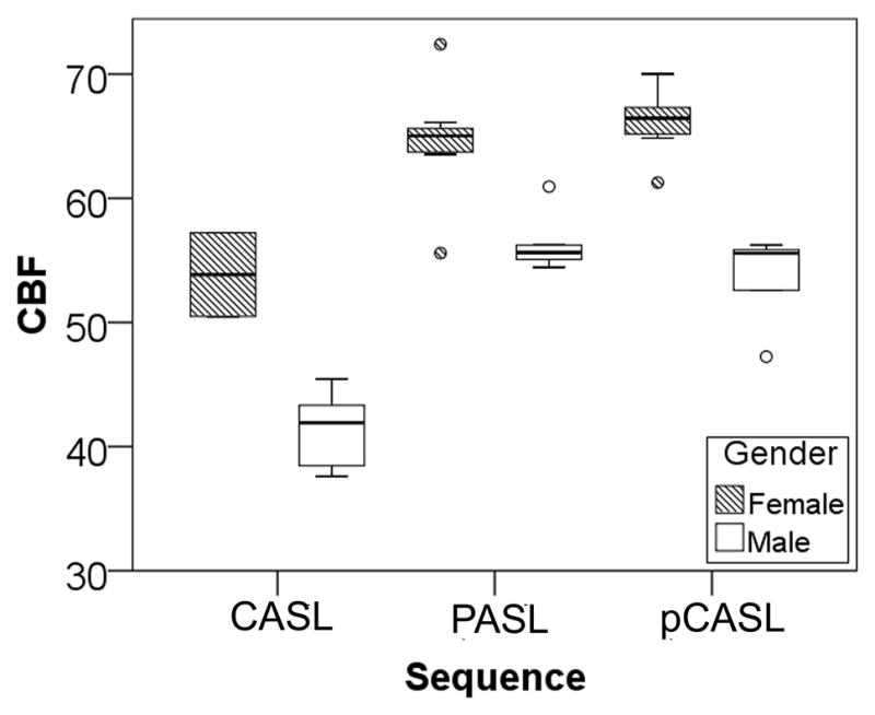
Box plot of male and female GM CBF values for the three sequences. For each group, the thick line inside the box represents the median, and the two ends of the box are the 1^st and 3^rd quartile. The T-bars for each box extend to 1.5 times the height of the box. Values that lie outside the T-bars are represented by circles and identified as outliers.

DISCUSSION

The mean ± SD GM CBF values obtained with all three sequences were in good agreement with prior ASL studies (11,19–21), as well as CBF estimates using ¹⁵O PET and ¹³³Xe (22–25). Interestingly, CBF estimates from CASL were significantly lower than CBF estimates from PASL and pCASL. One potential source of error is the assumed inversion efficiency of 0.68 for CASL, which was calculated from simulation results (13) and not actually measured in vivo. Moreover, since the labeling plane of CASL typically lies in the inhomogeneous region of the Tx/Rx head coil, it is possible that inversion efficiency may vary considerably between subjects. Given the high reproducibility of the pCASL scans of the current study, the pCASL data were used as a standard to estimate the inversion efficiency of the CASL scans and the mean CASL inversion efficiency thus calculated were 0.54 ± 0.13, 0.54 ± 0.10, 0.45 ± 0.07 and 0.50 ± 0.03 for the four scan sessions. While these lower estimates of inversion efficiency are potentially confounded by the technical instabilities encountered during the study with our Tx/Rx coil, and therefore cannot be generalized to all CASL experiments, the variability observed in these estimates highlight a potentially significant source of error for CASL on Tx/Rx coils.

For reproducibility assessment, the current study utilizes both wsCV and ICC for two reasons. Firstly, both are commonly reported in other studies, which makes it easier to compare results. Secondly, ICC is dependent on the between-subject variance, thus it may differ for different populations. The wsCV, on the other hand, provides an unbiased measurement of reproducibility since it is normalized to the mean of the measurements. As is evident from Tables 1 and 2, reproducibility declined with increasing rescan intervals for all three ASL variants. This result is not surprising, given how the three rescan intervals are sensitive to various contributions of error to the ASL experiment. The within-session reproducibility, primarily sensitive to scanner instabilities and errors induced by data processing, was indeed the highest. This was followed by the one-hour reproducibility, which includes repositioning errors. Finally, the one-week reproducibility, which includes both physiological fluctuations and repositioning errors, was the lowest. While prior studies have used similar experimental design to investigate ASL reproducibility at various scan intervals, few provide a direct comparison between multiple ASL variants at 3T. Compared to a similarly designed study at 3T using another PASL variant—QUASAR, which reported within-subject SDs of 3.1 (within-session), 4.3 (after repositioning) and 5.3 (after 13 days) ml/100g/min (26), results for PASL in the current study (3.8, 4.6 and 5.5 ml/100g/min) are in excellent agreement despite the different PASL sequences used for the two studies. Other PASL studies conducted at 1.5T have also reported similar wsCVs and ICCs (20,27). The lack of a substantial improvement in reproducibility with increasing field strength, despite the SNR gain, is evidence that physiological noise also scales with field strength (21,28). Thus while fewer averages may be required at high field strengths for accurate CBF quantification, reproducibility is still limited by physiological noise.

Despite the major contribution of physiological noise at one week, pCASL still has the lowest wsCV and highest ICC amongst the three sequences, indicating superior reproducibility. The high GM ICC associated with pCASL in the current study is in excellent agreement with a recent paper which reported the within session ICC for background-suppressed pCASL (29). But the WM ICC for our study is slightly lower. It is possible that background suppression is particularly beneficial for WM, which typically has lower perfusion signal and is therefore more sensitive to errors. Further investigation of the effects of background suppression on ASL repeatability is warranted. Another modification to pCASL that may affect its reproducibility is MP-pCASL (30), which uses multiple phase offsets instead of the standard two phase (180 for control and 0 for tag) approach to estimate off-resonance and gradient errors. While we did not directly compare the reproducibility of regular pCASL and MP-pCASL, our results do not indicate that regular pCASL suffers from additional sources of fluctuation compared to other ASL methods. In fact, pCASL had the highest reproducibility in the current study. A possible explanation for this apparent discrepancy may be vendor differences in pCASL implementation. Most prior pCASL studies were performed on GE scanners (5,30), which have different eddy current compensation schemes and also always scan at isocenter, which may affect the shimming at the labeling plane. Additional studies are needed to determine if MP-pCASL can further improve precision of pCASL measurements.

Of the three sequences, CASL demonstrated the poorest reproducibility for measurements made after subject repositioning. The range of wsCVs for the current study is roughly in agreement with prior studies on CASL reproducibility (31–33); however, Table 2 shows that regions supplied with the posterior circulation such as the PCA vascular territories, posterior cingulate and precuneus, have large wsCVs (up to 45.1%). Closer examination of the CBF maps revealed two subjects with very poor posterior circulation perfusion in one or more of the CASL scans (see Figure 6), which was not observed in the pCASL or PASL CBF maps of the same subjects. It is possible these subjects were positioned such that their PCAs were not at an optimal angle relative to the tagging plane, resulting in suboptimal tagging. Simulations have shown that AM-CASL is also particularly sensitive to variations in flow velocity compared to pCASL (34), likely due to incomplete double-inversion during the amplitude-modulated control. This sensitivity to flow velocity, in addition to the aforementioned variation in labeling efficiency due to the limited RF coverage of the Tx/Rx head coil, and the trend towards using high sensitivity array coils with body coil transmission, indicate that CASL has a diminishing role in future ASL studies.

Figure 6.

Sample CBF maps in ml/100g/min from all 7 subjects obtained using CASL. Notice two of the maps appear to have limited signal in portions of the posterior circulation (arrows).

Several limitations exist in the current study. First, we did not include a comparison with pulsed ASL methods using Look-Locker sampling of various inversion times such as QUASAR (35), in which CBF is calculated based on a “model-free” approach and transit time and arterial blood volume estimates in addition to CBF quantification. However, no pCASL and CASL equivalents have been implemented, which makes comparison between all of these methods difficult. Nonetheless, the PASL reproducibility estimates from the current study were in excellent agreement with those reported in a multi-site study using QUASAR (26), suggesting that the two quantification approaches do not have a major effect on the reproducibility of the CBF measurements. Secondly, we did not attempt to compare various quantification models, but instead used a simple single-blood-compartment model (36) for all three ASL methods. Parkes et al. have shown that the single-blood-compartment model provides a vast improvement in accuracy of CBF estimates compared to the single-tissue-compartment model, while eliminating the need to calculate an additional T₁ map required by the more complicated two-compartment model (37). A further simplification to the quantification process was to use assumed values of T1 and labeling efficiencies. Advantages to this approach include reduced scan time, as well as reduced measurement errors for these parameters, which could manifest as noise and reduce the reproducibility of CBF estimates. On the other hand, as is evident in our CASL data, deviation of these parameters from literature values lead to inaccuracies in CBF quantification. Thus it is important to consider the compromise between various quantification approaches on precision and reproducibility of ASL experiments. As a result of our quantification approach, results of the current study may not be completely applicable to ultra-high field strengths where blood and brain T₁ differences increase, nor to patient populations in whom T₁ values are altered.

In conclusion, our study demonstrates the excellent reproducibility of pCASL, which combines the advantages of both CASL and PASL methods, including the ability to use high sensitivity array coils, high SNR and tagging efficiency. This high precision makes pCASL an attractive method for CBF measurements in clinical settings. However, reproducibility of pCASL and PASL were comparable at longer scan intervals such as one week, suggesting that physiological noise is the primary limiting factor of ASL reproducibility at long intervals. Modifications such as background suppression and multi-phase pCASL, which focus on reducing physiological noise contributions, may further improve the performance of ASL.

References

- 1.Detre JA, Alsop DC. Perfusion magnetic resonance imaging with continuous arterial spin labeling: methods and clinical applications in the central nervous system. Eur J Radiol. 1999;30:115–124. doi: 10.1016/s0720-048x(99)00050-9. [DOI] [PubMed] [Google Scholar]
- 2.Wong EC, Buxton RB, Frank LR. A theoretical and experimental comparison of continuous and pulsed arterial spin labeling techniques for quantitative perfusion imaging. Magn Reson Med. 1998;40:348–355. doi: 10.1002/mrm.1910400303. [DOI] [PubMed] [Google Scholar]
- 3.Alsop DC, Detre JA. Multisection cerebral blood flow MR imaging with continuous arterial spin labeling. Radiology. 1998;208:410–416. doi: 10.1148/radiology.208.2.9680569. [DOI] [PubMed] [Google Scholar]
- 4.Hernandez-Garcia L, Lewis DP, Moffat B, Branch CA. Magnetization transfer effects on the efficiency of flow-driven adiabatic fast passage inversion of arterial blood. NMR Biomed. 2007;20:733–742. doi: 10.1002/nbm.1137. [DOI] [PMC free article] [PubMed] [Google Scholar]
- 5.Dai W, Garcia D, de Bazelaire C, Alsop DC. Continuous flow-driven inversion for arterial spin labeling using pulsed radio frequency and gradient fields. Magn Reson Med. 2008;60:1488–1497. doi: 10.1002/mrm.21790. [DOI] [PMC free article] [PubMed] [Google Scholar]
- 6.Wu WC, Fernandez-Seara M, Detre JA, Wehrli FW, Wang J. A theoretical and experimental investigation of the tagging efficiency of pseudocontinuous arterial spin labeling. Magn Reson Med. 2007;58:1020–1027. doi: 10.1002/mrm.21403. [DOI] [PubMed] [Google Scholar]
- 7.Wang J, Alsop DC, Song HK, et al. Arterial transit time imaging with flow encoding arterial spin tagging (FEAST) Magn Reson Med. 2003;50:599–607. doi: 10.1002/mrm.10559. [DOI] [PubMed] [Google Scholar]
- 8.Wong EC. Quantifying CBF with pulsed ASL: technical and pulse sequence factors. J Magn Reson Imaging. 2005;22:727–731. doi: 10.1002/jmri.20459. [DOI] [PubMed] [Google Scholar]
- 9.Parkes LM, Rashid W, Chard DT, Tofts PS. Normal cerebral perfusion measurements using arterial spin labeling: reproducibility, stability, and age and gender effects. Magn Reson Med. 2004;51:736–743. doi: 10.1002/mrm.20023. [DOI] [PubMed] [Google Scholar]
- 10.Kim SG. Quantification of relative cerebral blood flow change by flow-sensitive alternating inversion recovery (FAIR) technique: application to functional mapping. Magn Reson Med. 1995;34:293–301. doi: 10.1002/mrm.1910340303. [DOI] [PubMed] [Google Scholar]
- 11.Wong EC, Buxton RB, Frank LR. Quantitative imaging of perfusion using a single subtraction (QUIPSS and QUIPSS II) Magn Reson Med. 1998;39:702–708. doi: 10.1002/mrm.1910390506. [DOI] [PubMed] [Google Scholar]
- 12.Zhang Y, Song HK, Wang J, Techawiboonwong A, Wehrli FW. Spatially-confined arterial spin-labeling with FAIR. J Magn Reson Imaging. 2005;22:119–124. doi: 10.1002/jmri.20362. [DOI] [PubMed] [Google Scholar]
- 13.Wang J, Zhang Y, Wolf RL, Roc AC, Alsop DC, Detre JA. Amplitude-modulated continuous arterial spin-labeling 3.0-T perfusion MR imaging with a single coil: feasibility study. Radiology. 2005;235:218–228. doi: 10.1148/radiol.2351031663. [DOI] [PubMed] [Google Scholar]
- 14.Mugler JP, 3rd, Brookeman JR. Three-dimensional magnetization-prepared rapid gradient-echo imaging (3D MP RAGE) Magn Reson Med. 1990;15:152–157. doi: 10.1002/mrm.1910150117. [DOI] [PubMed] [Google Scholar]
- 15.Lu H, Clingman C, Golay X, van Zijl PC. Determining the longitudinal relaxation time (T1) of blood at 3.0 Tesla. Magn Reson Med. 2004;52:679–682. doi: 10.1002/mrm.20178. [DOI] [PubMed] [Google Scholar]
- 16.Tatu L, Moulin T, Bogousslavsky J, Duvernoy H. Arterial territories of the human brain: cerebral hemispheres. Neurology. 1998;50:1699–1708. doi: 10.1212/wnl.50.6.1699. [DOI] [PubMed] [Google Scholar]
- 17.Shrout PE, Fleiss JL. Intraclass correlations: uses in assessing rater reliability. Psychol Bull. 1979;86:420–428. doi: 10.1037//0033-2909.86.2.420. [DOI] [PubMed] [Google Scholar]
- 18.Bland JM, Altman DG. Measurement error proportional to the mean. BMJ. 1996;313:106. doi: 10.1136/bmj.313.7049.106. [DOI] [PMC free article] [PubMed] [Google Scholar]
- 19.Yang Y, Frank JA, Hou L, Ye FQ, McLaughlin AC, Duyn JH. Multislice imaging of quantitative cerebral perfusion with pulsed arterial spin labeling. Magn Reson Med. 1998;39:825–832. doi: 10.1002/mrm.1910390520. [DOI] [PubMed] [Google Scholar]
- 20.Yen YF, Field AS, Martin EM, et al. Test-retest reproducibility of quantitative CBF measurements using FAIR perfusion MRI and acetazolamide challenge. Magn Reson Med. 2002;47:921–928. doi: 10.1002/mrm.10140. [DOI] [PubMed] [Google Scholar]
- 21.Wang J, Alsop DC, Li L, et al. Comparison of quantitative perfusion imaging using arterial spin labeling at 1.5 and 4.0 Tesla. Magn Reson Med. 2002;48:242–254. doi: 10.1002/mrm.10211. [DOI] [PubMed] [Google Scholar]
- 22.Carroll TJ, Teneggi V, Jobin M, et al. Absolute quantification of cerebral blood flow with magnetic resonance, reproducibility of the method, and comparison with H2(15)O positron emission tomography. J Cereb Blood Flow Metab. 2002;22:1149–1156. doi: 10.1097/00004647-200209000-00013. [DOI] [PubMed] [Google Scholar]
- 23.Blauenstein UW, Halsey JH, Jr, Wilson EM, Wills EL, Risberg J. 133Xenon inhalation method. Analysis of reproducibility: some of its physiological implications. Stroke; a journal of cerebral circulation. 1977;8:92–102. doi: 10.1161/01.str.8.1.92. [DOI] [PubMed] [Google Scholar]
- 24.Frackowiak RS, Lenzi GL, Jones T, Heather JD. Quantitative measurement of regional cerebral blood flow and oxygen metabolism in man using 15O and positron emission tomography: theory, procedure, and normal values. Journal of computer assisted tomography. 1980;4:727–736. doi: 10.1097/00004728-198012000-00001. [DOI] [PubMed] [Google Scholar]
- 25.Grandin CB, Bol A, Smith AM, Michel C, Cosnard G. Absolute CBF and CBV measurements by MRI bolus tracking before and after acetazolamide challenge: repeatabilily and comparison with PET in humans. Neuroimage. 2005;26:525–535. doi: 10.1016/j.neuroimage.2005.02.028. [DOI] [PubMed] [Google Scholar]
- 26.Petersen ET, Mouridsen K, Golay X. The QUASAR reproducibility study, Part II: Results from a multi-center Arterial Spin Labeling test-retest study. Neuroimage. 49:104–113. doi: 10.1016/j.neuroimage.2009.07.068. [DOI] [PMC free article] [PubMed] [Google Scholar]
- 27.Jahng GH, Song E, Zhu XP, Matson GB, Weiner MW, Schuff N. Human brain: reliability and reproducibility of pulsed arterial spin-labeling perfusion MR imaging. Radiology. 2005;234:909–916. doi: 10.1148/radiol.2343031499. [DOI] [PMC free article] [PubMed] [Google Scholar]
- 28.Kruger G, Kastrup A, Glover GH. Neuroimaging at 1.5 T and 3.0 T: comparison of oxygenation-sensitive magnetic resonance imaging. Magn Reson Med. 2001;45:595–604. doi: 10.1002/mrm.1081. [DOI] [PubMed] [Google Scholar]
- 29.Xu G, Rowley HA, Wu G, et al. Reliability and precision of pseudo-continuous arterial spin labeling perfusion MRI on 3.0 T and comparison with 15O-water PET in elderly subjects at risk for Alzheimer’s disease. NMR Biomed. 2010;23:286–293. doi: 10.1002/nbm.1462. [DOI] [PMC free article] [PubMed] [Google Scholar]
- 30.Jung Y, Wong EC, Liu TT. Multiphase pseudocontinuous arterial spin labeling (MP-PCASL) for robust quantification of cerebral blood flow. Magn Reson Med. 2010 doi: 10.1002/mrm.22465. [DOI] [PubMed] [Google Scholar]
- 31.Floyd TF, Ratcliffe SJ, Wang J, Resch B, Detre JA. Precision of the CASL-perfusion MRI technique for the measurement of cerebral blood flow in whole brain and vascular territories. J Magn Reson Imaging. 2003;18:649–655. doi: 10.1002/jmri.10416. [DOI] [PubMed] [Google Scholar]
- 32.Gevers S, Majoie CB, van den Tweel XW, Lavini C, Nederveen AJ. Acquisition time and reproducibility of continuous arterial spin-labeling perfusion imaging at 3T. AJNR Am J Neuroradiol. 2009;30:968–971. doi: 10.3174/ajnr.A1454. [DOI] [PMC free article] [PubMed] [Google Scholar]
- 33.Hermes M, Hagemann D, Britz P, et al. Reproducibility of continuous arterial spin labeling perfusion MRI after 7 weeks. MAGMA. 2007;20:103–115. doi: 10.1007/s10334-007-0073-3. [DOI] [PubMed] [Google Scholar]
- 34.Pohmann R, Budde J, Auerbach EJ, Adriany G, Ugurbil K. Theoretical and experimental evaluation of continuous arterial spin labeling techniques. Magn Reson Med. 2010;63:438–446. doi: 10.1002/mrm.22243. [DOI] [PubMed] [Google Scholar]
- 35.Petersen ET, Lim T, Golay X. Model-free arterial spin labeling quantification approach for perfusion MRI. Magn Reson Med. 2006;55:219–232. doi: 10.1002/mrm.20784. [DOI] [PubMed] [Google Scholar]
- 36.Buxton RB. Quantifying CBF with arterial spin labeling. J Magn Reson Imaging. 2005;22:723–726. doi: 10.1002/jmri.20462. [DOI] [PubMed] [Google Scholar]
- 37.Parkes LM, Tofts PS. Improved accuracy of human cerebral blood perfusion measurements using arterial spin labeling: accounting for capillary water permeability. Magn Reson Med. 2002;48:27–41. doi: 10.1002/mrm.10180. [DOI] [PubMed] [Google Scholar]