Cryptic Evolution: Does Environmental Deterioration Have a Genetic Basis?

Abstract

Cryptic evolution has been defined as adaptive evolutionary change being masked by concurrent environmental change. Empirical studies of cryptic evolution have usually invoked a changing climate and/or increasing population density as the form of detrimental environmental change experienced by a population undergoing cryptic evolution. However, Fisher (1958) emphasized that evolutionary change in itself is likely to be an important component of “environmental deterioration,” a point restated by Cooke et al. (1990) in the context of intraspecific competition. In this form, environmental deterioration arises because a winning lineage has to compete against more winners in successive generations as the population evolves. This “evolutionary environmental deterioration” has different implications for the selection and evolution of traits influenced by resource competition than general environmental change. We reformulate Cooke's model as a quantitative genetic model to show that it is identical in form to more recent developments proposed by quantitative geneticists. This provides a statistical framework for discriminating between the alternative hypotheses of environmental change and environmental deterioration caused by evolutionary change. We also demonstrate that in systems where no phenotypic change has occurred, there are many reasonable biological processes that will generate patterns in predicted breeding values that are consistent with what has been interpreted as cryptic evolution, and care needs to be taken when interpreting these patterns. These processes include mutation, sib competition, and invisible fractions.

THE absence of microevolutionary change where it is expected is a long-standing problem in evolutionary biology (Merila et al. 2001b). The breeders' equation is the simplest model of evolutionary change for continuous characters and predicts evolutionary change when a heritable trait is under directional selection (Falconer 1983). Given that most traits are heritable (Lynch and Walsh 1998) and estimates indicate that selection is often directional (Kingsolver et al. 2001; Hereford et al. 2004; Perez and Munch 2010), we should expect evolutionary change to be observed much more often if the breeders' equation adequately captures the evolutionary process and estimates of selection and heritability are correct (Kinnison and Hendry 2001). Proposed solutions to this problem have usually invoked some correlated aspect of an individual's phenotype (Lande 1979; Price et al. 1988; Blows and Higgie 2003; Blows et al. 2004), a relative's phenotype (Kirkpatrick and Lande 1989), or the environment (Mitchell-Olds and Shaw 1987; Rausher 1992). Once these correlated “traits” are taken into account, the predicted genetic covariance between the trait and fitness may be reduced. Under a more general quantitative genetic model of evolutionary change (Robertson 1966) this genetic covariance is equal to the evolutionary response to selection. However, in long-term studies of wild systems it has been hard to identify correlated traits that can adequately explain the lack of evolutionary change often observed (Merila et al. 2001b).

A related hypothesis was proposed by Cooke et al. (1990), who suggested that evolutionary change may be occurring, but that its phenotypic consequences could be masked by concurrent environmental change. In their original model Cooke et al. (1990) suggested that a major component of this environmental change could be caused by the evolution of competitive ability in the population itself, resulting in “red queen” dynamics (Van Valen 1973). Although Cooke et al. (1990) suggested their results were an extension to Fisher's (1958) fundamental theorem, Frank and Slatkin (1992) convincingly argued that this process was subsumed within Fisher's concept of “environmental deterioration,” which had been widely misinterpreted. In this context, environmental deterioration arises because as the population evolves, a winning lineage has to compete against more winners in successive generations, resulting in a drop in relative fitness, a process that we call “evolutionary environmental deterioration.” However, Cooke et al. (1990) noted that they were not able to distinguish between evolutionary environmental deterioration and other forms of environmental change in their long-term data set on lesser snow geese (Anser caerulescens), because population density also increased over the study period. Subsequently, Merila et al. (2001a), using a quantitative genetics approach on a population of collared flycatchers (Ficedula albicolis), demonstrated that although the genetic component of “condition” increased over the study period, the environmental component decreased. Similar findings have been shown in other long-term vertebrate studies (Garant et al. 2004; Wilson et al. 2007) and have been called “cryptic evolution.” Although these studies often cite and even explicitly test Cooke et al.'s (1990) original model, they have invoked changes in population density and/or changes in climate as the source of environmental change, without considering the process that both Cooke et al. (1990) and Fisher (1958) emphasized as important: environmental deterioration as a result of evolutionary change. In addition, all of these studies have been on body-size–related traits that appear to be under consistent positive directional selection (Kingsolver and Pfennig 2004; Perez and Munch 2010). Whereas general environmental change would reduce body size only under certain scenarios, environmental change caused by the evolution of competitive ability would always act to reduce body size and may therefore likely be a more general explanation for why the body size of most species seems to be suboptimal despite being heritable (Blanckenhorn 2000).

In this article, we cast Cooke et al.'s (1990) model as a quantitative genetic model and clarify its meaning in terms of the multivariate breeders' equation. Using recent advances in statistical theory (Gianola and Sorensen 2004), we then show how evolutionary environmental deterioration can be distinguished from general environmental change in real data. We also show that in its most basic form Cooke et al.'s (1990) model is virtually identical to indirect genetic models derived in plant breeding (Griffing 1967) and more recently applied in animal breeding (Bijma et al. 2007a). However, since basic animal models have been used to test for cryptic evolution (Merila et al. 2001a; Garant et al. 2004; Wilson et al. 2007), we determine the conditions under which predicted breeding values from a basic animal model increase over time, but environmental deviations decrease over time, a pattern that has generally been considered as conclusive evidence of cryptic evolution (Postma 2006). We show that although these patterns are consistent with environmental deterioration, there are alternative biological processes that can give rise to such trends.

METHODS AND RESULTS

Evolutionary environmental deterioration and quantitative genetics:

Without loss of generality we use a simplified version of Cooke et al.'s (1990) model where the phenotype (υ₁) follows the model

(1)

where ɛ₁ and α₁ are, respectively, an environmental effect and a genetic effect that determine the conversion of resource R into υ₁. In Cooke et al.'s (1990) original model a second environmental deviation is included in the product, but is redundant for our purposes.

The amount of resource available to an individual is determined by

(2)

Here the fraction A/N is the amount of the total resource (A) available to an individual when the resource is shared evenly over all individuals (N is the population size). The second fraction determines the ability of an individual to obtain more or less than its fair share, where the trait υ₂ can be viewed as competitive ability and the overbar denotes the expectation. When there is no variation in competitive ability, then this fraction is unity and the resource is evenly split.

As with the first trait, the competitive ability is assumed to follow a multiplicative quantitative genetic model:

(3)

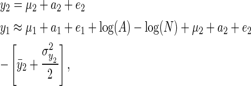
The model can be transformed into the more standard additive quantitative genetic model by working on the log scale (y₁ = log(υ₁))

(4)

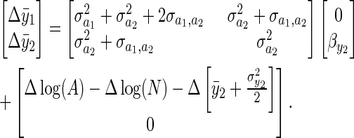
where μ₁ and μ₂ are trait-specific intercepts. The approximation is due to . We can get an expression for the total change in the mean of the two traits by combining the genetic response to selection based on the multivariate breeders' equation (Lande 1979) with the expression for environmental change (see also Iwasa and Pomiankowski 1991):

(5)

The first term on the right-hand side (RHS) is the familiar multivariate breeders' equation (Lande 1979) where the matrix is the additive genetic covariance matrix for the two traits, and the vector is a vector of directional selection gradients. We assume that although there is direct selection to acquire more resources , the allocation of those resources is already optimized and not under directional selection . The second term on the RHS captures “environmental” change, although it should be understood that environmental change in y₁ includes change induced by change in the mean value of y₂, which itself may be due to a genetic response to selection.

If we assume that the population size is large enough that the covariance between population-level properties of y₂ and an individual's breeding value or environmental deviation are negligible, and that change in the higher-order moments of y₂ are also small , Equation 5 can be simplified:

(6)

The term can be interpreted as Robertson's (1966) genetic covariance between a trait and fitness. To see how this interpretation can be given, decompose fitness (W) into a component predicted by y₂ and a residual e_W:

(7)

The covariance between y₁ and fitness within a generation can then be decomposed into a genetic and environmental covariance assuming residuals are uncorrelated with breeding values:

(8)

Designating Robertson's (1966) genetic covariance as S_G, we have

(9)

where S_G is equal to evolutionary change in the absence of environmental deterioration (Robertson 1966), and Δ log(A) and Δ log(N) are changes in environmental quality and population density, respectively. Cooke et al. (1990) put special emphasis on as a source of environmental deterioration, and Frank and Slatkin (1992) showed that this quantity is closely linked to Fisher's (1958) concept of environmental deterioration (see also Price 1972b; Ewens 1989). However, Cooke et al. (1990) indicated that Δ log(N) was also positive during the course of their study and so the effect of changes in population size could not be distinguished from environmental deterioration caused by the evolution of competitive ability. More recent studies have considered only the role of environmental change in terms of changes in population density (N) (Larsson et al. 1998; Wilson et al. 2007) or changes in environmental quality (A) (Merila et al. 2001a) or both (Garant et al. 2004), without considering the final term in Equation 9: evolutionary environmental deterioration.

A test for evolutionary environmental deterioration—a recursive quantitative genetic model:

The ability to acquire resources (y₂) or the total amount of resources available (A) is usually not measured, so we ask whether it is possible to distinguish between environmental change and evolutionary environmental deterioration given information on y₁ only. To illustrate the point we assume discrete annual generations in which all individuals interact equally, but emphasize that the model generalizes to more complex scenarios.

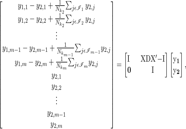
The model presented above can be expressed as a recursive quantitative genetic model (Gianola and Sorensen 2004) since one of the response variables (y₂) directly affects the other (y₁). Following Gianola and Sorensen (2004) we can rearrange Equation 4 such that the traits appear on the left-hand side (LHS) and the unknown parameters appear on the RHS,

(10)

where b are year effects that include the effects of between-year variation in A on the expression of y₁. k_i indexes the year in which individual i was present and ℐ_i the set of all individuals present in that year (including i itself). The LHS of Equation 10 for all individuals, nesting individuals within traits, can be represented in a more manageable matrix form, where X is an incidence matrix relating individuals to years, and D is a diagonal matrix with reciprocal annual population sizes along the diagonal,

(11)

where m is the total number of individuals across all years. The matrix on the RHS of Equation 11 is the structural coefficient matrix (Λ) of Gianola and Sorensen (2004), and it can be shown (appendix a) that the marginal distribution of y₁ (after marginalizing y₂) is given by

(12)

where B = XDX′, A is the additive genetic relatedness matrix, and and .

When there is no variance in the ability to acquire resources , the model coincides with the standard animal model that has been used to test for cryptic evolution (see below). The marginal distribution of the full model, however, has a similar form to that under Willham's (1972) maternal effect model (see p. 573 of Sorensen and Gianola 2002), as was noted by Bijma et al. (2007a) for their model of indirect genetic effects. In fact, this model coincides with Bijma et al.'s (2007a,b) model under the null hypothesis proposed by Hadfield and Wilson (2007), that the more individuals you interact with the less effect you can have on any one individual, and hence the matrix of reciprocal population sizes D. The only slight difference is that an individual also affects itself (by using up its own resources) whereas in Bijma et al.'s (2007a,b) model the indirect effect (called associative effect following Griffing 1967) caused by expression of y₂ is felt only by other individuals.

Each element of the matrix BAB has the form , where the expectation is the mean relatedness between individuals in i's year and j's year. This implies that two individuals should be more similar if their respective competitors are more closely related and therefore similar in competitive ability.

The term is harder to understand and implies that the expected covariance between individual i and individual j's phenotype is proportional to the mean relatedness of i to the individuals alive in j's year plus the mean relatedness of j to the individuals alive in i's year (E [r_i,ℐj] + E [r_j,ℐi]). If the genetic covariance between competitive ability and the allocation of resources to the focal trait (y₁) is zero, then this implies that two individuals should be less similar when they interact with each other's relatives. To see how this arises, imagine the extreme situation where individual i interacts only with j's relatives and individual j interacts only with i's relatives. If individual i is a better competitor than the relatives of j, then it will have a large phenotype. If competitive ability is heritable, then on average relatives of i are likely to outcompete individual j and cause its phenotype to be small.

A similar phenomenon arises at the environmental level when the environmental covariance between competitive ability and the allocation of resources to the focal trait is zero. The term B then implies that individuals who interact should resemble each other less because if individual i takes more resource, this leaves less for j. This effect decreases as populations become large because the effect of individual i on j's phenotypes will become diluted. More flexible relationships between population density and the strength of competition could be entertained (Hadfield and Wilson 2007; Bijma 2010c).

On the basis of these results we suggest that a test for evolutionary environmental deterioration should first involve estimating the indirect genetic (co)variances determined above . If these are found to be different from zero, then showing that the breeding value for competitive ability has increased would be consistent with evolutionary environmental deterioration.

The conditions for the pattern of cryptic evolution:

Above we have argued that general environmental change and evolutionary environmental deterioration—as envisaged by Cooke et al. (1990) and Frank and Slatkin (1992)—are separate and distinct processes. Evolutionary environmental deterioration depends on the presence of indirect effects, both genetic (Wolf et al. 1998) and environmental, arising from competition. To date, these indirect effects have not been included in models used to test for cryptic evolution. Rather models of the form

(13)

have generally been used, and individual predictions of breeding values and environmental deviations have been obtained using best linear unbiased prediction (BLUP). When the BLUP breeding values and BLUP environmental deviations from these models change in different directions over time, it is generally assumed that this is good evidence of cryptic evolution (Postma 2006). If the model defined by Equation 13 is the correct model, then the trends in BLUP breeding values and BLUP environmental deviations are unbiased estimators of the trends in actual breeding values and actual environmental deviations, although care has to be taken with hypothesis testing (Hadfield et al. 2010). However, if the model defined by Equation 13 is not the correct model, then predicted and actual trends may not coincide. In this section we determine the conditions under which fitting the basic animal model (Equation 13) would result in predicted trends that are consistent with what has been interpreted as cryptic evolution. We use these results to show that evolutionary environmental change does give rise to predicted trends that are consistent with the process, despite the model being wrong (i.e., Equation 13 is different from Equation 12). However, we also show that there are other biological processes not explicitly modeled that would also result in similar patterns.

To understand the statistical properties of estimators of evolutionary genetic change it is necessary to explicitly consider the process of selection, and Gianola et al. (1988) pointed out that to understand selection adequately the pedigree must be treated as a random variable rather than a fixed quantity. To be able to do this we consider the joint distribution of pedigrees and phenotypes when pedigrees consist of parents and their full-sib families and let the number of sibs in each family depend on the phenotypes of the parents. We then ask what properties of this joint distribution would give rise to predictions that have been treated as evidence of cryptic evolution.

Under the assumption that the mean phenotype has not changed between the parental and the offspring generation, we find that a positive trend in predicted breeding values and a negative trend in predicted environmental effects will result when

(14)

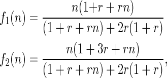
(see appendixes a–c for further details), where Δz is the deviation, midoffspring phenotype minus midparent phenotype (). Expectations are taken over families (as in Price's 1972a equation), each of which has two parents but a variable number of n offspring. The functions f₁(n) and f₂(n) are monotonic positive functions of parental fitness,

(15)

where r is the ratio . We had little success in simplifying the analysis or extending it to more general scenarios, but some insights can be gained from inequality (14), which we illustrate and validate with simulations of more complex pedigrees.

Because the functions are monotonic functions of parental fitness, the sign of the covariances will be the same as if parental fitness was used directly. If we assume directional selection on the trait is either absent or positive (i.e., the RHS is equal to or greater than zero) then any process that either (a) reduces E[Δz] or (b) reduces the covariance between Δz and parental fitness could give rise to patterns in predicted breeding values that have been interpreted as evidence of cryptic evolution.

Example 1—sib effects:

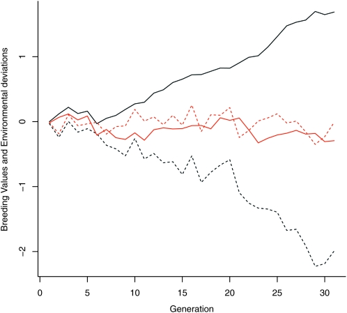
General changes within families (E[Δz]) may be the result of between-generation changes in the environment such as environmental deterioration (Frank and Slatkin 1992), but there are also other mechanisms. For example, under a neutral model most parents have more sibs than their offspring (see appendixes a–c) and so any effect of family size on offspring phenotype can cause a general difference between parent and offspring phenotype. To illustrate, we made a simple simulation with discrete generations (30), a constant population size (100), and no selection on phenotype. Individuals formed monogamous pairs at random, and family sizes were generated from a Poisson distribution with a mean of exp(2) = 7.4. The resulting offspring were sampled at random to form the following generation, and their phenotypes were simulated according to

(16)

where is offspring i's parental fitness (i.e., the number of sibs individual i has). The residual (e_i) was simulated from a standard normal distribution, and the breeding value (a_i) from a normal distribution with a mean equal to the average breeding value of i's parents and a variance equal to half the additive genetic variance, which was also set to 1 (i.e., r = = 1). is the effect that an increase in sibship size has on an individual's phenotype which we set to 0.5. A simple animal model was fitted using the resulting pedigree and phenotype data, and breeding values were predicted. Across 100 replications the average change in the true breeding values was small and nonsignificant (0.017 ± 0.060, P = 0.775) but the change in predicted breeding value was large (2.229 ± 0.042, P < 0.001). Figure 1 shows the actual trend in breeding values (and environmental deviations over time) in gray, and the predicted trends in black, for a typical simulated run. There are some traits for which positive values of are likely, for example, chicks from larger broods often beg more (e.g., Neuenschwander et al. 2003), but there are as yet no published studies of cryptic evolution for this type of trait. For traits that are negatively affected by sib competition, such as body size, is likely to be negative and the primary motivation for using a positive coefficient is to be consistent (i.e., to obtain positive rather than negative trends in predicted breeding values). Reversing the sign of the coefficient results in a decrease in predicted breeding values and an increase in environmental deviations which could potentially mask the signature of cryptic evolution.

Figure 1.—

Simulated breeding values (solid gray line) and environmental deviations (dashed gray line) when interacting with more sibs increases phenotypic value. Shown are predicted breeding values (solid black line) and predicted environmental deviations (dashed black line) for the same data using the basic animal model.

Example 2—the invisible fraction:

In addition to general changes within families (E[Δz]) as exemplified above, any process that reduces the covariance between Δz and parental fitness more than that expected under a standard quantitative genetic model could also give rise to patterns in predicted breeding values that have been interpreted as cryptic evolution. In the above example, this covariance will be positive and will in part counteract the effects of the negative E[Δz]. However, other mechanisms can generate negative covariances. For example, mutations affecting body size in Caenorhabditis elegans tend to reduce rather than increase size (Azevedo et al. 2002). If these mutations act proportionally rather than additively, then the same mutation affecting offspring of large worms will tend to reduce body size more than in offspring of small worms. If body size is under positive selection, then these mutations would give rise to negative covariances between parental fitness and Δz.

It is also important to realize that parental fitnesses and parental/offspring phenotypes are not necessarily the real values, but the values that went into the analysis. If small parents tend not to be observed (for example, sneaky males are not identified), then the offspring of single parents tend to be smaller than expected under the assumption of random mating, which is assumed in the basic model. Likewise, Mojica and Kelly (2010) show that although large flowers confer a fecundity advantage in Mimulus guttatus, larger-flowered genotypes have greater mortality prior to trait expression and so their flower size goes unmeasured. Under this scenario, correlative studies will tend to measure a smaller-sized subset of offspring from large parents, resulting in Δz values that negatively covary with measured parental fitness (fecundity). The subset of unmeasured dead individuals has been termed the invisible fraction (Grafen 1988) and is known to cause problems for the estimation of quantitative genetic parameters (Im et al. 1989). Here we show that this form of missing data is sufficient to generate trends in predicted breeding values that resemble patterns that would be obtained from cryptic evolution.

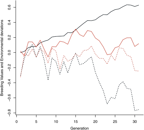
Again, we made a simple simulation with discrete generations (30) and a constant population size (100) in which individuals with a propensity to produce large flowers (y) have a reduced chance of surviving to maturity (and therefore being measured) but conditional on flowering have higher fecundity. Family sizes were generated from a Poisson distribution,

(17)

where individual j is i's mate, and β_f is the fecundity selection gradient that was set to 0.2. The phenotypes of individuals were generated according to the basic quantitative genetic model

(18)

However, the probability of an individual surviving to adulthood (and therefore being measured) was proportional to the density of y in a normal distribution with mean equal to and a variance of γ. S is the deviation from the optima of the population mean in that year and was set to −0.2, and γ is equivalent to the strength of stabilizing selection around the optima, which was set to 1.75. These parameters result in a selection regime where fecundity selection and viability selection are approximately equal.

Again, a simple animal model was fitted using the resulting pedigree and phenotype data, and breeding values were predicted. Across 100 replications the average change in the true breeding values was small and nonsignificant (−0.006 ± 0.046, P = 0.893) but the change in predicted breeding values was large (0.953 ± 0.018, P < 0.001). Figure 2 shows the actual trend in breeding values (and environmental deviations over time) in gray, and the predicted trends in black, for a typical simulated run.

Figure 2.—

Simulated breeding values (solid gray line) and environmental deviations (dashed gray line) when survival and fecundity selection balance. Shown are predicted breeding values (solid black line) and predicted environmental deviations (dashed black line) for the same data using the basic animal model. In both cases, individuals that failed to survive were not included in the analysis.

DISCUSSION

In this article we clarify the original meaning of environmental deterioration (Fisher 1958; Cooke et al. 1990; Frank and Slatkin 1992) by placing it in the context of quantitative genetics. By doing this, we show that previous quantitative genetic studies in wild systems (Merila et al. 2001a; Garant et al. 2004; Wilson et al. 2007) ignored the process of evolutionary environmental deterioration that Fisher (1958) and particularly Cooke et al. (1990) had emphasized as important (Frank and Slatkin 1992).

Evolutionary environmental deterioration in the sense used by Cooke et al. (1990) arises because as genotypes that confer greater competitive ability spread, the amount of resources available to other genotypes diminishes. When the amount of resource is fixed, this leads to a zero-sum game whereby the mean resource acquired remains constant, and the mean trait value does not change despite underlying evolutionary change (Dickerson 1955; Griffing 1967; Wolf 2003). Moreover, the share of the resource acquired by the superior genotypes diminishes as they spread because they end up competing with themselves, making it more difficult to observe the phenotypic effects of superior genotypes. Because it is this information that is used to detect evolutionary environmental deterioration in the statistical procedure outlined in this article, we acknowledge that power may be low (Bijma 2010a). Greater success may be had with laboratory- or field-based time-shift experiments that are able to measure individuals in environments characteristic of earlier or later generations, as is done in studies of host–parasite coevolution (Gaba and Ebert 2009).

In a recent article, Hadfield et al. (2010) showed that current methods for detecting cryptic evolution are highly anticonservative and that the evidence for cryptic evolution in two of the published examples (Garant et al. 2004; Wilson et al. 2007) was weak. However, it should be understood that the estimates of evolutionary change are conditional on the model used and that by obtaining the marginal distribution of the data under Cooke's model, we show that models previously used to demonstrate cryptic evolution are the wrong models if evolutionary environmental change is the main cause of any environmental deterioration. However, it would be possible to obtain estimates of evolutionary change under a model of evolutionary environmental deterioration and test them appropriately. In this article we took, as Cooke et al. (1990) did, a simplified pedagogical model where all individuals in a year interact to the same degree. We acknowledge that this is ecologically naive and that to obtain more accurate and more powerful estimates of this evolutionary process it is undoubtedly necessary to work with systems where groups of interacting individuals can be defined or the level of interaction between different individuals quantified. In many systems, interacting individuals will be relatives and we stress that in obtaining Equation 6 the simplifying assumption that the covariance between an individual's breeding value and the mean breeding value of the group is zero precludes a response to kin selection that can and should be included (Bijma 2010b; McGlothlin et al. 2010). In addition, Cooke et al.'s (1990) model assumes that competitive abilities are transitive in the sense that if individual A outcompetes B, and individual B outcompetes C, then individual A must outcompete individual C (Harris et al. 2008). Such a model predicts that individuals in later generations would on average outcompete individuals in previous generations, which may hold over short timescales but is unlikely to be a general property of competitive interactions, as evidenced in yeast (Paquin and Adams 1983). Furthermore, it is important to recognize that even if patterns consistent with cryptic evolution are found, there are other biological processes that may be responsible for them. For example, because groups that share more relatives are likely to be close in time, any temporal autocorrelation in environmental effects may be wrongly interpreted as indirect genetic effects. Here, using a simplified full-sib model we have derived conditions under which a conclusion of cryptic evolution might be drawn from the basic animal model and find that sibling competition, selection bias, and mutation could all cause patterns that are equally consistent with this interpretation.

However, as noted above, our formulation of Cooke et al.'s (1990) model is virtually identical to indirect genetic effect models (Griffing 1967) recently applied to livestock data (Bijma et al. 2007a). These models have been used to demonstrate the influence of indirect genetic effects in poultry and pigs, where groups of interacting individuals can be readily defined as those animals sharing a cage or a pen (e.g., Bijma et al. 2007b; Bergsma et al. 2008). Bijma et al. (2007b) have argued that negative covariance between direct and indirect genetic effects can be interpreted as arising from heritable variation in competitive ability and should constrain phenotypic responses to selection among individuals (Griffing 1967). Selection experiments that have explicitly considered indirect genetic effects have yielded results supporting this prediction (e.g., Goodnight 1985; Muir 2005). This source of constraint and the phenomenon of evolutionary environmental deterioration discussed here are one and the same. Given the potential importance of competition and resource limitation in natural populations, we believe the conditions that would give rise to evolutionary environmental deterioration are widespread. However, it is currently difficult to assess the potential magnitude of such effects without a better idea of the amount of additive genetic variance in competitive ability that segregates under natural conditions in wild populations. Thus while we certainly expect unequivocal demonstration of cryptic evolution by evolutionary environmental deterioration to be difficult, the importance of resource-dependent trait expression for many aspects of an organism's phenotype makes this an interesting, if challenging, topic for further study in wild systems.

APPENDIX A: SIMPLIFYING THE RECURSIVE QG MODEL

The structural coefficient matrix has the inverse

(A1)

using Equation 14 (Searle 2006, p. 260).

Modifying Equation 29 of Gianola and Sorensen (2004), we get the marginal distribution of ,

(A2)

assuming each individual is present only in a single year.

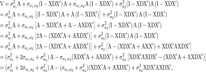
Since X′X is a diagonal matrix of population sizes and D is a diagonal matrix of reciprocal population sizes, X′XD is an identity matrix, and the above equation simplifies:

(A3)

Also (I − XDX′)(μ₂ + 0) = 0 since , and

(A4)

which gives

(A5)

APPENDIX B: THE CONDITIONS FOR THE PATTERN OF CRYPTIC EVOLUTION

The pedigree consists of F full-sib families, with midparental values and midoffspring values z′ taken on n offspring. The vector of individual phenotypes is denoted as y and z with E[y] = E[z] (i.e., there is no phenotypic trend), and we wish to find the conditions under which a trend in predicted breeding values is positive but masked by an annual environmental trend (b_y > b_z).

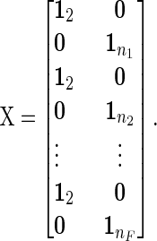
Grouping individuals by family, with parents first, the records are associated with the year of measurement by the incidence matrix:

(B1)

With full-sib families A⁻¹ has the structure

(B2)

and so has the form

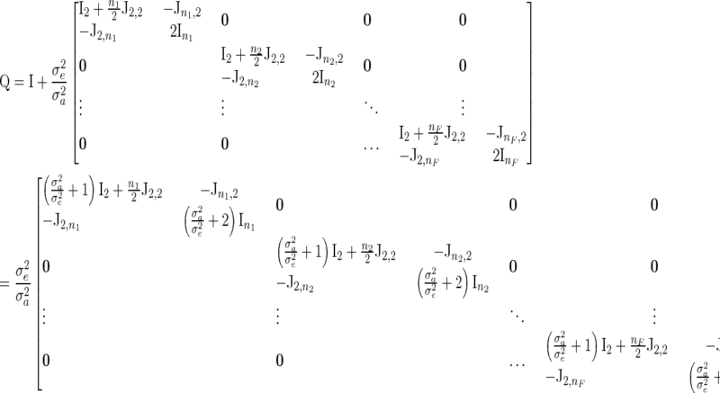(B3)

giving

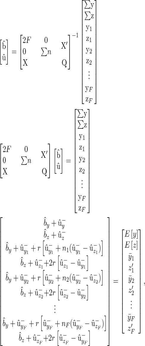(B4)

where .

Since , by definition, E[y] = b_y,

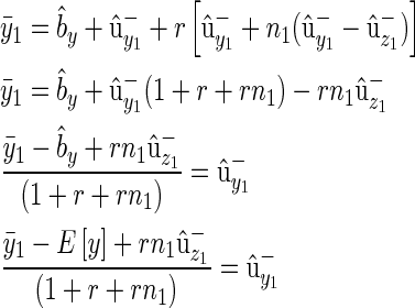(B5)

and

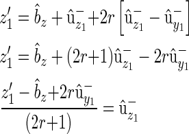(B6)

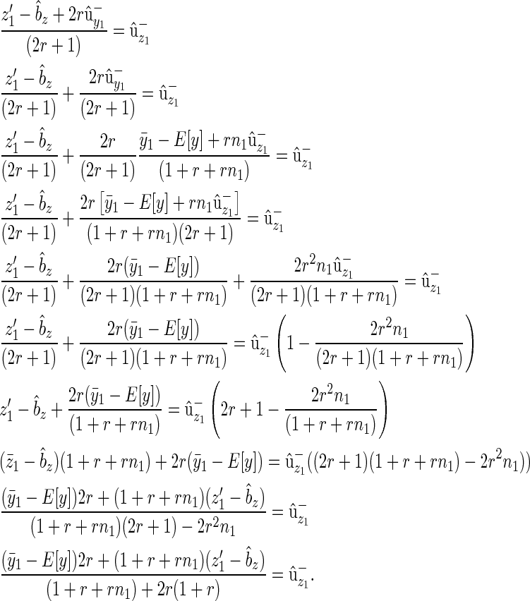
with substitution

(B7)

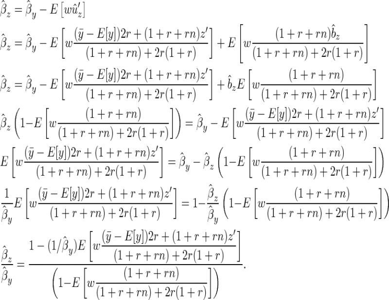
Since , where the expectation is over families and is the relative fitness of the parents,

(B8)

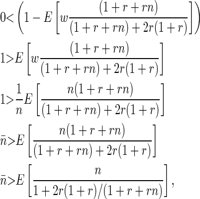
The denominator is positive when

(B9)

which is always true if r > 0 (which it is by definition), since 2r(1 + r)/(1 + r + rn) must be positive.

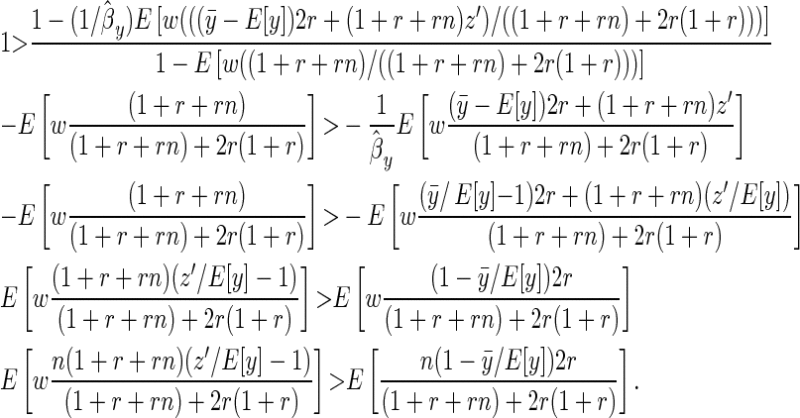
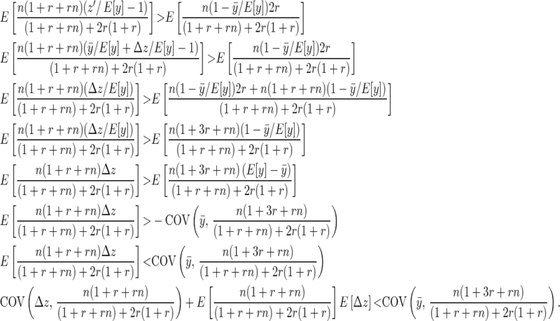
Given these results we want to know the conditions under which () assuming E[y] > 0:

(B10)

We can rewrite the family mean as , where Δz is the deviation of the offspring mean from the midparental value, and noting that ,

(B11)

APPENDIX C: WHY MOST PARENTS HAVE MORE SIBS THAN THEIR OFFSPRING UNDER A NEUTRAL MODEL

To show why parents on average will often have more sibs than their offspring we take the example of an asexual population. In generation 1 individual i has n_i offspring and n_i,j grandoffspring through their jth offspring. We denote population size in each generation as Ng, , and , where the subscripts g, p, and o indicate quantities taken over individuals in generation 1 (grandparents), generation 2 (parents), and generation 3 (offspring), respectively.

Our aim is to give the conditions under which parents, on average, have more sibs than their offspring,

(C1)

where δ = 1 if an individual breeds and 0 otherwise, and s is the number of sibs it has and s′ the number of sibs its offspring has. We subscript E with g, p or o to indicate the individuals over which the expectation is taken. s′ − s is not defined if an individual does not breed, and hence the condition δ > 0,

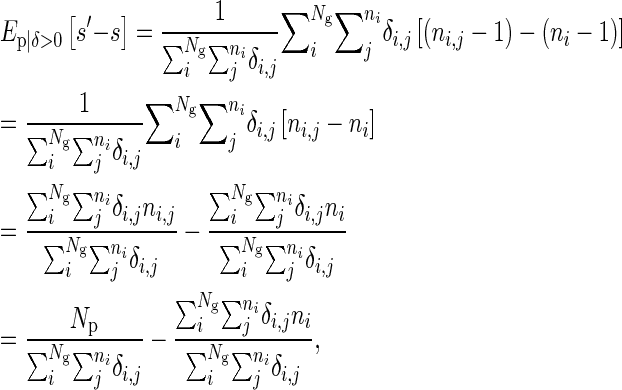(C2)

since the number of sibs an individual has is one less than the number of offspring its parents had.

This implies

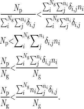(C3)

is the number of i's offspring that breed, and so denoting b_i as the proportion of individual i's offspring that breed we have and

(C4)

If we assume the parental and offspring reproductive functions are independent, then COV_g(n², b) = 0 and E_g[b] = 1 − f_p(0), where f_p is the probability mass function for the distribution of offspring from individuals in generation p. Given the assumption of independence, we need to give the conditions under which

(C5)

Here we show that this will be the case for some common distributions when population size is constant and the distribution of offspring in different generations is identically distributed.

For the Poisson distribution, we have

(C6)

For a multinomial distribution with each parent having equal probability of success,

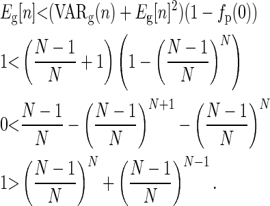(C7)

Since , then the above is satisfied if , which is true if N ≥ 2.

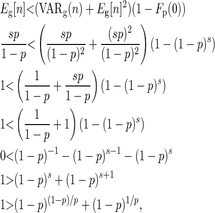
For a negative binomial distribution reproduction is the sum of a series of reproductive bouts where an offspring is (success) or is not (failure) produced. , where p is the probability of success in any one bout, and s is the number of failures before stopping reproduction, and

(C8)

which is satisfied when p ≠ 0 and p ≠ 1.

References

- Azevedo, R. B. R., P. D. Keightley, C. Laurén-Määttä, L. L. Vassilieva, M. Lynch et al., 2002. Spontaneous mutational variation for body size in Caenorhabditis elegans. Genetics 162 755–765. [DOI] [PMC free article] [PubMed] [Google Scholar]
- Bergsma, R., E. Kanis, E. F. Knol and P. Bijma, 2008. The contribution of social effects to heritable variation in finishing traits of domestic pigs (Sus scrofa). Genetics 178 1559–1570. [DOI] [PMC free article] [PubMed] [Google Scholar]
- Bijma, P., 2010. a Estimating indirect genetic effects: precision of estimates and optimum designs. Genetics 186 1013–1028. [DOI] [PMC free article] [PubMed] [Google Scholar]
- Bijma, P., 2010. b Fisher's fundamental theorem of inclusive fitness and the change in fitness due to natural selection when conspecifics interact. J. Evol. Biol. 23 194–206. [DOI] [PubMed] [Google Scholar]
- Bijma, P., 2010. c Multilevel selection 4: modeling the relationship of indirect genetic effects and group size. Genetics 186 1029–1031. [DOI] [PMC free article] [PubMed] [Google Scholar]
- Bijma, P., W. A. Muir and J. A. M. Van Arendonk, 2007. a Multilevel selection 1: quantitative genetics of inheritance and response to selection. Genetics 175 277–288. [DOI] [PMC free article] [PubMed] [Google Scholar]
- Bijma, P., W. M. Muir, E. D. Ellen, J. B. Wolf and J. A. M. Van Arendonk, 2007. b Multilevel selection 2: estimating the genetic parameters determining inheritance and response to selection. Genetics 175 289–299. [DOI] [PMC free article] [PubMed] [Google Scholar]
- Blanckenhorn, W. U., 2000. The evolution of body size: What keeps organisms small? Q. Rev. Biol. 75 385–407. [DOI] [PubMed] [Google Scholar]
- Blows, M. W., and M. Higgie, 2003. Genetic constraints on the evolution of mate recognition under natural selection. Am. Nat. 161 240–253. [DOI] [PubMed] [Google Scholar]
- Blows, M. W., S. F. Chenoweth and E. Hine, 2004. Orientation of the genetic variance-covariance matrix and the fitness surface for multiple male sexually selected traits. Am. Nat. 163 E329–E340. [DOI] [PubMed] [Google Scholar]
- Cooke, F., P. D. Taylor, C. M. Francis and R. F. Rockwell, 1990. Directional selection and clutch size in birds. Am. Nat. 136 261–267. [Google Scholar]
- Dickerson, G. E., 1955. Genetic slippage in response to selection for multiple objectives. Cold Spring Harbor Symp. Quant. Biol. 20 213–224. [DOI] [PubMed] [Google Scholar]
- Ewens, W. J., 1989. An interpretation and proof of the fundamental theorem of natural-selection. Theor. Popul. Biol. 36 167–180. [DOI] [PubMed] [Google Scholar]
- Falconer, D., 1983. Introduction to Quantitative Genetics. Longman, New York.
- Fisher, R. A., 1958. The Genetical Theory of Natural Selection, Ed. 2. Dover, New York.
- Frank, S. A., and M. Slatkin, 1992. Fisher's fundamental theorem of natural selection. Trends Ecol. Evol. 7 92–95. [DOI] [PubMed] [Google Scholar]
- Gaba, S., and D. Ebert, 2009. Time-shift experiments as a tool to study antagonistic coevolution. Trends Ecol. Evol. 24 226–232. [DOI] [PubMed] [Google Scholar]
- Garant, D., L. E. B. Kruuk, R. H. McCleery and B. C. Sheldon, 2004. Evolution in a changing environment: a case study with great tit fledging mass. Am. Nat. 164 E115–E129. [DOI] [PubMed] [Google Scholar]
- Gianola, D., and D. Sorensen, 2004. Quantitative genetic models for describing simultaneous and recursive relationships between phenotypes. Genetics 167 1407–1424. [DOI] [PMC free article] [PubMed] [Google Scholar]
- Gianola, D., S. Im and R. L. Fernando, 1988. Prediction of breeding value under Henderson's selection model—a revisitation. J. Dairy Sci. 71 2790–2798. [Google Scholar]
- Goodnight, C. J., 1985. The influence of environmental variation on group and individual selection in a cress. Evolution 39 545–558. [DOI] [PubMed] [Google Scholar]
- Grafen, A., 1988. On the uses of data on lifetime reproductive success, pp. 454–471 in Reproductive Success, edited by T. H. Clutton-Brock. University of Chicago Press, Chicago.
- Griffing, B., 1967. Selection in reference to biological groups. I. Individual and group selection applied to populations of unordered groups. Aust. J. Biol. Sci. 20 127–139. [PubMed] [Google Scholar]
- Hadfield, J. D., and A. J. Wilson, 2007. Multilevel selection 3: modelling the effects of interacting individuals as a function of group size. Genetics 177 667–668. [DOI] [PMC free article] [PubMed] [Google Scholar]
- Hadfield, J., A. J. Wilson, D. Garant, B. C. Sheldon and L. E. B. Kruuk, 2010. The misuse of BLUP in ecology and evolution. Am. Nat. 175 116–125. [DOI] [PubMed] [Google Scholar]
- Harris, W. E., A. J. McKane and J. B. Wolf, 2008. The maintenance of heritable variation through social competition. Evolution 62 337–347. [DOI] [PubMed] [Google Scholar]
- Hereford, J., T. F. Hansen and D. Houle, 2004. Comparing strengths of directional selection: How strong is strong? Evolution 58 2133–2143. [DOI] [PubMed] [Google Scholar]
- Im, S., R. L. Fernando and D. Gianola, 1989. Likelihood inferences in animal breeding under selection—a missing-data theory view point. Genet. Sel. Evol. 21 399–414. [Google Scholar]
- Iwasa, Y., and A. Pomiankowski, 1991. The evolution of costly mate preferences. 2. The handicap principle. Evolution 45 1431–1442. [DOI] [PubMed] [Google Scholar]
- Kingsolver, J. G., and D. W. Pfennig, 2004. Individual-level selection as a cause of Cope's rule of phyletic size increase. Evolution 58 1608–1612. [DOI] [PubMed] [Google Scholar]
- Kingsolver, J. G., H. E. Hoekstra, J. M. Hoekstra, D. Berrigan, S. N. Vignieri et al., 2001. The strength of phenotypic selection in natural populations. Am. Nat. 157 245–261. [DOI] [PubMed] [Google Scholar]
- Kinnison, M. T., and A. P. Hendry, 2001. The pace of modern life II: from rates of contemporary microevolution to pattern and process. Genetica 112 145–164. [PubMed] [Google Scholar]
- Kirkpatrick, M., and R. Lande, 1989. The evolution of maternal characters. Evolution 43 485–503. [DOI] [PubMed] [Google Scholar]
- Lande, R., 1979. Quantitative genetic analysis of multivariate evolution, applied to the brain: body size allometry. Evolution 33 402–416. [DOI] [PubMed] [Google Scholar]
- Larsson, K., H. P. van der Jeugd, I. T. van der Veen and P. Forslund, 1998. Body size declines despite positive directional selection on heritable size traits in a barnacle goose population. Evolution 52 1169–1184. [DOI] [PubMed] [Google Scholar]
- Lynch, M., and B. Walsh, 1998. Genetics and Analysis of Quantitative Traits. Sinauer Associates, Sunderland, MA.
- McGlothlin, J. W., A. J. Moore, J. B. Wolf and E. D. Brodie, 2010. Interacting phenotypes and the evolutionary process. III. Social evolution. Evolution 64 2558–2574. [DOI] [PubMed] [Google Scholar]
- Merila, J., L. E. B. Kruuk and B. C. Sheldon, 2001. a Cryptic evolution in a wild bird population. Nature 412 76–79. [DOI] [PubMed] [Google Scholar]
- Merila, J., B. C. Sheldon and L. E. B. Kruuk, 2001. b Explaining stasis: microevolutionary studies in natural populations. Genetica 112 199–222. [PubMed] [Google Scholar]
- Mitchell-Olds, T., and R. G. Shaw, 1987. Regression analysis of natural selection: statistical inference and biological interpretation. Evolution 41 1149–1161. [DOI] [PubMed] [Google Scholar]
- Mojica, J. P., and J. K. Kelly, 2010. Viability selection prior to trait expression is an essential component of natural selection. Proc. R. Soc. B Biol. Sci. 277 2945–2950. [DOI] [PMC free article] [PubMed] [Google Scholar]
- Muir, W. M., 2005. Incorporation of competitive effects in forest tree or animal breeding programs. Genetics 170 1247–1259. [DOI] [PMC free article] [PubMed] [Google Scholar]
- Neuenschwander, S., M. W. G. Brinkhof, M. Kolliker and H. Richner, 2003. Brood size, sibling competition, and the cost of begging in great tits (Parus major). Behav. Ecol. 14 457–462. [Google Scholar]
- Paquin, C. E., and J. Adams, 1983. Relative fitness can decrease in evolving asexual populations of S. cerevisiae. Nature 306 368–371. [DOI] [PubMed] [Google Scholar]
- Perez, K. O., and S. B. Munch, 2010. Extreme selection on size in the early lives of fish. Evolution 64 2450–2457. [DOI] [PubMed] [Google Scholar]
- Postma, E., 2006. Implications of the difference between true and predicted breeding values for the study of natural selection and micro-evolution. J. Evol. Biol. 19 309–320. [DOI] [PubMed] [Google Scholar]
- Price, G. R., 1972. a Extension of covariance selection mathematics. Ann. Hum. Genet. 35 485–490. [DOI] [PubMed] [Google Scholar]
- Price, G. R., 1972. b Fisher's ‘fundamental theorem’ made clear. Ann. Hum. Genet. 36 129–140. [DOI] [PubMed] [Google Scholar]
- Price, T., M. Kirkpatrick and S. J. Arnold, 1988. Directional selection and the evolution of breeding date in birds. Science 240 798–799. [DOI] [PubMed] [Google Scholar]
- Rausher, M. D., 1992. The measurement of selection on quantitative traits—biases due to environmental covariances between traits and fitness. Evolution 46 616–626. [DOI] [PubMed] [Google Scholar]
- Robertson, A., 1966. A mathematical model of culling process in dairy cattle. Anim. Prod. 8 95–108. [Google Scholar]
- Sorensen, D., and D. Gianola, 2002. Likelihood, Bayesian and MCMC Methods in Quantitative Genetics (Statistics for Biology and Health). Springer-Verlag, New York.
- Van Valen, L., 1973. A new evolutionary law. Evol. Theory 1 1–30. [Google Scholar]
- Willham, R. L., 1972. The role of maternal effects in animal breeding: Iii. Biometrical aspects of maternal effects in animals. J. Anim. Sci. 35 1288–1293. [DOI] [PubMed] [Google Scholar]
- Wilson, A. J., J. M. Pemberton, J. G. Pilkington, T. H. Clutton-Brock, D. W. Coltman et al., 2007. Quantitative genetics of growth and cryptic evolution of body size in an island population. Evol. Ecol. 21 337–356. [Google Scholar]
- Wolf, J. B., 2003. Genetic architecture and evolutionary constraint when the environment contains genes. Proc. Natl. Acad. Sci. USA 100 4655–4660. [DOI] [PMC free article] [PubMed] [Google Scholar]
- Wolf, J. B., E. D. Brodie, J. M. Cheverud, A. J. Moore and M. J. Wade, 1998. Evolutionary consequences of indirect genetic effects. Trends Ecol. Evol. 13 64–69. [DOI] [PubMed] [Google Scholar]