Abstract
Complex genetic interactions lie at the foundation of many diseases. Understanding the nature of these interactions is critical to developing rational intervention strategies. In mammalian systems hypothesis testing in vivo is expensive, time consuming, and often restricted to a few physiological endpoints. Thus, computational methods that generate causal hypotheses can help to prioritize targets for experimental intervention. We propose a Bayesian statistical method to infer networks of causal relationships among genotypes and phenotypes using expression quantitative trait loci (eQTL) data from genetically randomized populations. Causal relationships between network variables are described with hierarchical regression models. Prior distributions on the network structure enforce graph sparsity and have the potential to encode prior biological knowledge about the network. An efficient Monte Carlo method is used to search across the model space and sample highly probable networks. The result is an ensemble of networks that provide a measure of confidence in the estimated network topology. These networks can be used to make predictions of system-wide response to perturbations. We applied our method to kidney gene expression data from an MRL/MpJ × SM/J intercross population and predicted a previously uncharacterized feedback loop in the local renin–angiotensin system.
MULTIFACTORIAL experiments performed with a randomized experimental design provide conditions for uncovering causation (Fisher 1926). In populations derived from inbred strain crosses, the genetic variation that occurs naturally within a population serves as a multifactorial perturbation (Jansen and Nap 2001). Randomization of alleles during meiosis ensures the unidirectional influence of genotype on phenotype, allowing for the identification of quantitative trait loci (QTL) causal to phenotypes. Expression quantitative trait loci (eQTL) data consist of genotypes at markers across the genome, genome-wide gene expression, and other phenotypes. Identifying causal relationships between complex traits from eQTL data has recently become a topic of great interest (Rockman 2008; Li et al. 2010).
QTL can act as causal anchors to distinguish direct and indirect relationships between pairs of phenotypes (Li et al. 2006). Conditional independence tests among triplets (two phenotypes and a shared QTL) have been widely used to sort out causal, reactive, and independent relationships between pairs of phenotypes (Schadt et al. 2005). These methods have been extended to allow for the interaction between genotype and phenotype (Kulp and Jagalur 2006). The TRIGGER algorithm was developed for large-scale inference using conditional independence tests to generate networks at a desired false discovery rate (Chen et al. 2007). In another approach, an undirected network is estimated using only continuous phenotypes and QTL are added and used to direct the edges in the network (Chaibub-Neto et al. 2008). Bayesian Network (BN) methodology has been previously implemented with structural priors derived from QTL analysis and the conditional analysis of triplets (Zhu et al. 2004, 2007). Many current approaches are based on the local analysis of small sets of variables that are pieced together from multiple causality tests between phenotypes. This can be problematic because local relationships between variables can be altered in the context of a larger network of interactions.
Recently methodologies have emerged for the joint modeling of genotypes (discrete variables) and phenotypes (continuous variables). A method that employs simulated annealing and Markov chain Monte Carlo (MCMC) methods was proposed and applied to dynamic data (Winrow et al. 2010). A method called QTLnet uses a modified Metropolis–Hastings algorithm to estimate the QTL network conditional on a proposed phenotype network (Chaibub-Neto et al. 2010).
In this article we describe a Bayesian approach to the joint inference of the genotype–phenotype map from eQTL data. We define local models in which a child node representing a continuous phenotype is causally connected to parent nodes that may be discrete (genotypes) or continuous (phenotypes) and describe their relationships through hierarchical regression models, which can accommodate interaction terms. We derive a scoring metric for evaluating local models and place constraints on the network through a structural prior. A search procedure designed for efficient graph sampling is proposed. We have applied our method to expression data from the kidneys of an MRL/MpJ × SM/J intercross to infer causal relationships among genes known to react in the renal renin–angiotensin system (RAS).
METHODS
Statistical model and sampling strategy:
Bayesian networks are graphical models that leverage conditional independencies between variables to describe joint multivariate probability distributions (Heckerman 1997). Network nodes correspond to discrete or continuous random variables and edges represent variable dependencies. We define the data as
 |
where X and Q are the sets of random variables representing phenotypes and genotypes at QTL markers, respectively.
The graph G is restricted to be a directed acyclic graph (DAG). G obeys the Markov condition, which states that, each variable, Di, is independent of its nondescendants (unconnected), given its parents in G. Under these assumptions, the joint probability distribution can be conveniently decomposed into the product
 |
(1) |
where πG(Di) is the set of parents of Di in G. The posterior probability of the graph G after the data D is taken into account and can be written as the product of the structural prior P(G) and the marginal likelihood P(D|G):
 |
The marginal likelihood requires integration over the parameters θ,
 |
where P(θ|G) is the prior on the parameters for a given graph structure. The DAG restriction permits factorization of the marginal likelihood according to Equation 1.
Identifying the DAG that best explains the data is a nondeterministic polynomial-time hard (NP-hard) problem. We impose structural priors to constrain the model space and apply a search procedure to sample highly probable graphs. Following Imoto et al. (2004), we express prior knowledge through an energy function
 |
where B is the prior matrix with elements  that express the prior probability that there is a causal edge from node Xi to node Xj. The prior distribution takes the form of an energy function embedded in a Gibbs distribution,
 |
where τ is referred to as the inverse temperature hyperparameter. The prior parameter matrix can be thought of as a Gaussian belief network where the indexes bi,j represent the strength of the dependency between variables Xi and Xj (Heckerman 1997). The energy function measures the Manhattan distance between the belief network and the graph at hand. In our applications, we enforce a noninformative prior by setting B = 0m×n and τ = 0.1, which promotes sparsity by penalizing dense graphs. In principle, biological knowledge of the graph structure from previous experiments and literature can be encoded into this framework, but this is outside the scope of this article (Werhli and Husmeier 2007).
The computational intensity of the sampling scheme necessitates an additional constraint on parent cardinalities. We enforce a fan-in restriction of at most k parents for every node in the network. In our applications we set k = 3. For each child node we enumerate and precompute scores for all possible parent sets, penalizing for more complex graph structures.
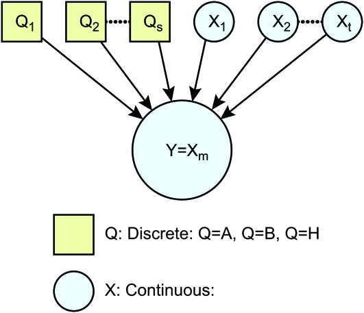
We define a local family to be a child node and its parents (Figure 1) and model them with multilevel regression models (Gelman and Hill 2007). Consider the general case, when a continuous child node y = Xm has parents πG(y) = {Q1, … , Qk, X1, … , Xn}. We use the model
 |
where β0 is constant,  and
and  . The model in matrix notation is given by
 |
where A ∈ Rn×k, y, ɛ ∈ Rn, and β ∈ Rk. The columns of A correspond to a constant term, a binary matrix indicating genotypes for each parental Qj, and columns for each parental Xi. In our formulation, we set a diffuse prior by assuming the mean effects are all the same. This can be modified to reflect available a priori information about the QTL effects.
Figure 1.—
Example of a local family, where continuous child node y = Xm has discrete and continuous parents πG(y) = {Q1, Q2, … , Qs, X1, X2, … , Xt}.
For convenience, we make the assumption that unknown parameters of local probability distributions are independent and utilize the normal and inverse gamma distributions, which are conditionally conjugate. In addition, we assume that the prior distribution of the parameters for local models depends only on the parents (parameter modularity). For a local model, the joint distribution for the parameters is
 |
where
 |
 |
The parameters a and b can be thought of as carrying information from a prior experiment, where a is the number of observations and b = λa/(a − 1) is the prior estimate of σ2 (George and McCulloch 1993). Small values for a and b can convey ignorance about the parameters. Notably, as a, b → 0, the posterior does not have a proper limiting distribution, and posterior inference has been shown to be sensitive (Dongen 2006; Gelman 2006). We use values between 10−3 and 10−1 and have not encountered any instability. In our experience, changing the values of a and b does have an effect on the precomputed scores, but overall the sampled networks do not change much. The resulting marginal likelihood for a model G is given by
 |
where p is the dimension of the parameter vector β, n is the sample size, and |·| is the determinant (Ntzoufras 2009).
The posterior sum of squares, SSpost, is defined as
 |
where the posterior estimates of β and σ are
 |
 |
The regression matrix A is typically ill-conditioned and can give rise to unstable parameter estimates. We implement a Tikhonov regularization scheme that stabilizes the least-squares problem and penalizes the curvature of the solution (Hansen 1998; Calvetti et al. 2006). The least-squares solution for the regression parameters  is obtained by solving the following minimization problem,
 |
where L2 is the discrete approximation of the second derivative,
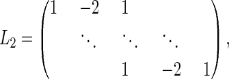 |
and λ is a Tikhonov regularization parameter. For convenience, in the global model (full graph), we omit reference to the regression matrix A, as it is implicit in the local graph structures Gk. The score ϕ for a local family Gk can be calculated as
 |
where Gk is the model that contains parents  . The posterior distribution for the full DAG can be calculated as the product of scores for local regression models:
 |
We implement a Metropolis–Hastings strategy to sample networks from the posterior distribution. Single edge proposals of adding, deleting, or reversing an edge in the current graph are known to not mix well and are slow to converge (Madigan and York 1995). The reversible edge (REV) proposal takes into account whether the reversal of an edge is useful in combination with the other nodes in the parent sets (Grzegorczyk and Husmeier 2008). The REV move reverses the edge between two nodes and then samples new parent sets such that the new graph structure is acyclic. We propose a combination of modified edge reversals and single-edge proposals for the discrete-continuous domain that arises in eQTL data (supporting information, File S1). This adaptation is restricted to edge reversals between continuous nodes, thereby preserving the unidirectional relationship between genotype and phenotype. Although the modified REV move operates only between continuous nodes (phenotypes), the genotype topology can be substantially changed indirectly through the re-estimation of the parent sets. All calculations are done in Matlab and the code is available upon request.
Applications:
Simulation study:
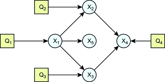
We simulated five continuous phenotypes and four discrete QTL (Figure 2) for intercross populations of size 500 using R/QTL (Broman and Sen 2009). The genome consists of five chromosomes of length 100, with 10 genetic markers randomly distributed across each chromosome. Phenotypes X1, X2, X3, and X4 have one QTL each on chromosomes 1, 2, 3, and 4, respectively, and phenotype X5 has no QTL. The QTL are unlinked and occur near the center of the chromosome. Additive and dominance effects were generated from U[0.5, 1] and U[0, 0.5], respectively. Phenotypes were generated from a normal distribution X ∼ N(0, 1) and were then modified according to a conditional Gaussian distribution,
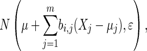 |
to preserve the structural relationships shown in Figure 2. The regression coefficients, bi,j, were fixed at  , and the variance, ɛ, was of the order of 1e − 1.
Figure 2.—
The simulated network was generated as the compilation of local models.
MRL/MpJ × SM/JF2 intercross:
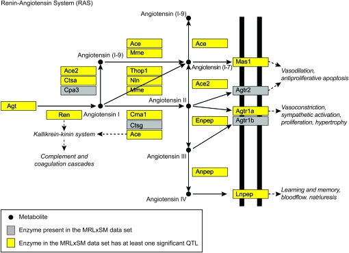
We applied our methods to kidney eQTL data from an MRL/MpJ × SM/J intercross (Figure S1; Hageman et al. 2011). Pathway enrichment analysis revealed the RAS pathway (Figure 3) as overrepresented (P-value <0.001) in the chromosome 4 trans-band. Of 18 genes in this pathway, 7 have a QTL in the chromosome 4 region, all of which were trans-regulated (Table S1). We identified 7 additional genes in this pathway that have at least one significant QTL elsewhere in the genome. These 14 genes, along with SNPs corresponding to significant QTL, were selected as variables. In cases with more than one significant SNP per chromosome, the SNP corresponding to the highest LOD score was selected (Table S2). These data are available in NCBI's Gene Expression Omnibus under accession no. GSE23310 (Edgar et al. 2002).
Figure 3.—
The RAS pathway as depicted in KEGG was overrepresented in the chromosome 4 trans-band for the MRL/MpJ × SM/J intercross. Members of this pathway with significant QTL are indicated. These enzymes and QTL were selected as network variables.
RESULTS AND DISCUSSION
We have proposed a Bayesian statistical framework for the joint inference of the causal phenotype–genotype network from the natural genetic variation in segregating populations. Networks are decomposed into local models with continuous children and scored using a Bayesian posterior probability. Structural priors that can encode sparsity and biological knowledge are used to constrain the model space. The modified Metropolis–Hastings algorithm relies on a single edge and reversible edge proposals for efficient DAG sampling. The result is an ensemble of highly probable networks from which predictions can be made.
In the simulation study, four chains were run from different random initial DAGs for 50,000 iterations for each data set. The acceptance rate in all cases was between 21% and 33%, and the reduction of scale parameters was <1.2 (Gilks et al. 1996). The initial burn-in was discarded, and the chains were combined for Bayesian model averaging (BMA) over graphs of high probability (Madigan and Raferty 1984). For each simulated data set, the BMA result is a matrix with entries that are estimates of the marginal probability of an edge (e.g., Table S3). To summarize this information, we compare the posterior probabilities for the causal relationship, Xi → Xj, and reactive relationship Xj → Xi for each phenotype. If there is a negligible difference (<0.05), we conclude that we are unable to establish the nature of relationship Xi ↔ Xj. To determine whether the relationships between QTL and phenotypes were adequately recovered, for each simulation we identified the parental QTL with the maximum posterior probability for each phenotype. The number of times features were recovered across the 100 simulated data sets is given in Table 1. Overall, our method performed well recovering both direct and indirect relationships from simulated data. The edges between QTL and phenotype were easier to recover than the edges between phenotypes. We struggled to identify the relationship between X1 and X5, which share a common QTL; however, this may be inherent to the structure of the model.
TABLE 1.
The number of times that each possible causal relationship had the highest posterior probability (top) and number of times that the causal QTL had the highest posterior probability (bottom)
| Phenotypes | → | ← | ←→ |
|---|---|---|---|
| (X1, X2) | 94 | 0 | 6 |
| (X1, X3) | 92 | 0 | 8 |
| (X1, X5) | 9 | 16 | 75 |
| (X2, X4) | 100 | 0 | 0 |
| (X3, X4) | 100 | 0 | 0 |
| QTL–phenotypes | → | ||
| (Q1, X1) | 86 | ||
| (Q2, X2) | 100 | ||
| (Q3, X3) | 100 | ||
| (Q4, X4) | 100 |
The RAS pathway plays a major role in blood pressure regulation (Fyhrquist and Saijonmaa 2008). Both systemic RAS and the activation of local tissue RAS have been associated with hypertension, diabetes, and cardiovascular and renal damage. We selected this pathway to demonstrate our approach on real kidney data from an F2 intercross. Our data, and hence our models, reflect only the local (renal) RAS, which is different from the more commonly referred to systemic RAS. The local RAS is not a closed system and can interact with the endocrine RAS as well as other peptide systems outside the kidney that are not considered here.
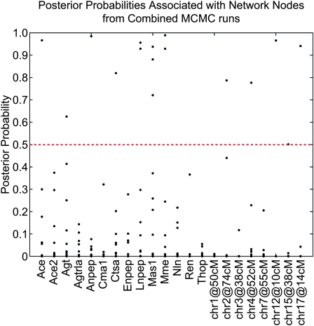
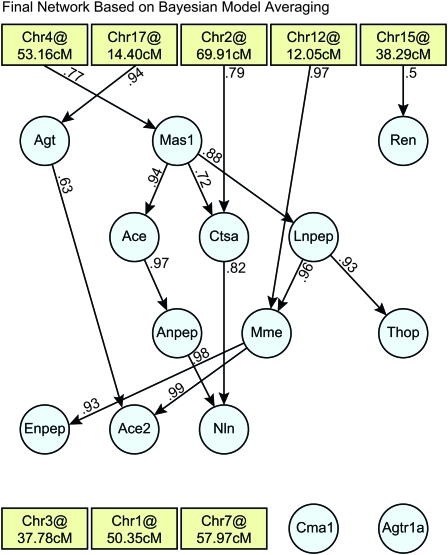
We applied our method to a reduced RAS pathway with 14 genes that have significant QTL somewhere in the genome. Two parallel chains were seeded from random DAGs and run for 800,000 iterations. Acceptance rates were 10% and 13%. The initial burn-in was discarded. The estimated posterior probabilities of the parameters (edges) were in strong agreement (ρ = 0.99), indicating convergence (Figure S2), and the distribution of posterior probabilities was clearly bimodal. Edges with probabilities >0.5 were selected for the final network on the basis of BMA (Figure 4). The posterior probabilities for all edges are given in Table S4. Alternatively, we employed model selection to extract the four most probable networks (Figure S3 and Figure S4).
Figure 4.—
Posterior probabilities estimated by BMA for each network node. Each point is an entry in the consensus matrix, which represents the probability of a connection associated with the given node. Connections with probabilities >0.5 serve as nodes in the final weighted network.
Our final model (Figure 5) differs from the canonical pathway (Figure 3), suggesting enzyme regulation in regions of the pathway that are not directly linked. For example, Mas1, which encodes the MAS1 oncogene and binds the angiotensin II metabolite angiotensin(1–7), has a large effect on Lnpep. Lnpep encodes the leucyl/cystinyl aminopeptidase, a receptor for another angiotensin II metabolite. The expression of Lnpep affects the expression of both Thop1 and Mme, both encoding enzymes that produce angiotensin(1–7), the ligand for the MAS1 oncogene. This relationship suggests a feedback loop in the canonical pathway. Mas1 appears to be a master regulator; we predict that intervention at this level will perturb nearly all pathway members with the exception of Ren and Agt. Ren was found to be causally linked to Mme with low probability (0.366); however, Mme is upstream of Ren with probability 0.245 (Table S4). We believe that Ren and Mme are causally linked, but the direction of causality is unclear. The actions of Ren likely do not occur at the transcriptional level.
Figure 5.—
A graphical representation of the final RAS network based on BMA. Edges were drawn if their probability exceeded 0.5.
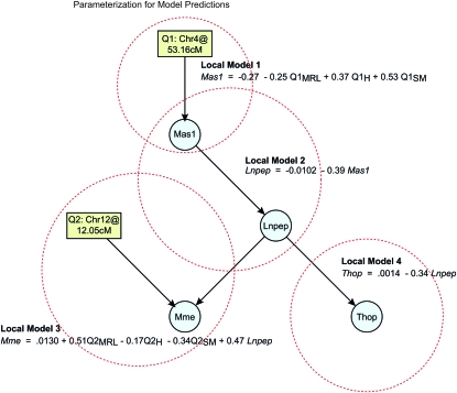
A major feature of this approach is the ability to generate hypotheses and perform in silico experiments with the networks. The Markov property allows us to consider each local family as independent of its predecessors. From the BMA network the most probable connections can be determined. Once a network is identified it can be parameterized by the regression coefficients of the local families. In the parameterized network, the sign and magnitude of the regression coefficients reveal the nature of the relationships between variables, and forward quantitative predictions can be made by simulation. We parameterized a highly probable region of the BMA network for the RAS pathway that involved Mas1, Lnpep, Mme, Thop, and QTL on chromosomes 4 and 12 (Figure 6). Examination of the regression coefficients suggests Mas1 inhibits the Lnpep receptor, which in turn inhibits Thop. The expression of Mme depends on the expression of Lnpep, but also the genotype on the chromosome 4 locus, e.g., Mme is strongly activated by a homozygous MRL genotype at the chromosome 4 locus. Further testing is required to validate these hypotheses. Nonetheless, our method provides a framework for predicting the effects of interventions, such as drugs, that attempt to modify gene action to alter downstream phenotypes.
Figure 6.—
An illustration of the parameterization of local models for the purpose of making forward prediction. The parameterization is given by the least-squares estimates of the regression coefficients for the local models; they provide insight into the relationships between network variables. We selected a highly probable region of the graph, which suggests a feedback mechanism in the canonical pathway.
The size of the model space grows at a superexponential rate with the number of nodes (Friedman et al. 2000), and adequate coverage of the model space becomes difficult and quickly impossible with increasing numbers of variables. These issues are inherent in BN methodologies. Even with the addition of the reversible-edge proposal, our method can reconstruct networks only on the order of 30 nodes before becoming unstable. This is a far stretch from the number of transcripts in an eQTL data set (≈30,000). The small sample size compared to the number of measured traits (n ≫ p) that arises in eQTL data is another limiting consideration. Variable selection is a major challenge for any network inference method. We found that restriction to a moderate number of biologically motivated variables is required for reliable inference and tractable sampling. A method that can infer mixed-domain dynamic BNs up to 10,000 nodes has been proposed (Winrow et al. 2010), but it is difficult to assess the validity of such large-scale networks. We are currently investigating improvements to our sampling scheme and priors that will allow us to infer larger systems, but we expect to achieve only modest increases.
QTLnet is an algorithm similar to our approach that uses homogeneous conditional Gaussian regression models and a hybrid Metropolis–Hastings algorithm to estimate network connections (Chaibub-Neto et al. 2010). In the QTLnet sampling scheme, a phenotype network is generated via single-edge proposals, and then the genetic architecture is estimated conditional on the proposed network. A combination of single-edge proposals and conditional genome scans makes QTLnet computationally intensive. We have applied both QTLnet (version 0.4.1) and our algorithm to the RAS pathway data (Figure S10, Figure S11, and Table S5). Both methods predict many of the same connections, including the identification of Mas1 as a master regulator and feedback in the canonical pathways between Mas1, Lnpep, Mma, and Thop. With no sparsity restrictions, QTLnet predicted a much denser set of interactions, which was expected. When we extended the number of variables by including gene expression data on RAS components that did not have QTL, our method provided essentially the same network (Figure S5, Figure S6, Figure S7, Figure S8, Figure S9, and Table S6). The QTLnet algorithm did not exhibit the same concordance (Figure S10, Figure S11, and Table S5); we found that genes with no significant QTL in the single-trait analysis were connected in the network, with the exception of Agtr1b.
An advantage of the QTLnet method is that it estimates unobserved QTL genotypes conditional on SNP markers using hidden Markov models (HMM) and conditions on them in the sampling process (Broman and Sen 2009). In contrast, we use selected SNPs for QTL in the model space. Therefore, the QTLnet model space is always smaller than ours, which eases the sampling process. On the other hand, conditional genome scans are performed and single-edge proposals are made, making iterations more laborious. A disadvantage of the QTLnet approach is the potential for more than one variable in a close genomic region (e.g., small regions on the same chromosome) to be represented in the network. Genotypes in close regions are not necessarily independent and their inclusion can affect the inferred topology. In our QTLnet-derived RAS networks, there are several instances of this; e.g., in the reduced RAS network there are two SNPs on chromosome 2 that are represented at 73 and 88 cM (Figure S11). The optimal way to include genotypes to safeguard against errors in inference due to linkage between variables in the causal network remains an open question.
We have adopted a structural prior in the form of a Gaussian belief network that has the potential to encode biological knowledge and sparsity. The sparsity prior that we applied can safeguard against overfitting, which is often an issue in a high-dimensional model space. Growing resources of publicly available data together with annotations from the literature can offer support for relationships between variables. However, methods for encoding this information into a prior belief network remain to be developed.
The interaction between genotype and phenotype has been shown to play an important role in the causal inference of network interactions (Kulp and Jagalur 2006). We have modeled the local relationships between continuous children with mixed parents using hierarchical regression models. These models can be extended to investigate the interaction between variables, i.e., phenotype–genotype, genotype–genotype, and phenotype–phenotype. However, the addition of interaction terms will substantially increase the search space. Such models may be feasible for small-scale networks.
In summary, we have proposed a Bayesian statistical framework for estimation of causal phenotype–genotype networks. Our method utilizes precomputed Bayesian scores of local models, structural priors, which can convey sparsity and biological knowledge, and an efficient MCMC search strategy. The resulting sample of highly probable networks can be mined for the discovery of novel phenotype relationships and predictions. Future developments need to address the preselection of variables and efficient search strategies; these issues are challenging and possibly insurmountable. There are growing resources of data that can provide knowledge about the expected interactions. Summarizing these data as a biologically informative prior distribution is not straightforward, but has the potential to substantially improve network inference. Computational methods for network inference are valuable tools for generating and validating hypotheses, which can drive new experiments.
Acknowledgments
This project was funded by grants from the National Institute of General Medical Sciences (GM076468) (to G.A.C. and R.K.); a National Heart, Lung, and Blood Institute NSRA fellowship (1F32HL095240-02) (to R.S.H.); an American Heart Association postdoctoral fellowship (to M.S.L.); and National Heart, Lung, and Blood Institute grants HL077796 and HL081162 (to B.P.).
Supporting information is available online at http://www.genetics.org/cgi/content/full/genetics.110.123273/DC1.
Available freely online through the author-supported open access option.
Sequence data from this article have been deposited with the National Center for Biotechnology Information's Gene Expression Omnibus Data Library under accession no. GSE23310.
References
- Broman, K. W., and S. Sen, 2009. A Guide to QTL Mapping With R/qtl. Springer-Verlag, Berlin/Heidelberg, Germany/New York.
- Calvetti, D., J. P. Kaipio and E. Somersalo, 2006. Aristotelian prior boundary conditions. Int. J. Math. Comput. Sci. 1 63–81. [Google Scholar]
- Chaibub-Neto, E., C. T. Ferrara, A. D. Attie and B. S. Yandell, 2008. Inferring causal phenotype networks from segregating populations. Genetics 179 1089–1100. [DOI] [PMC free article] [PubMed] [Google Scholar]
- Chaibub-Neto, E., M. P. Keller, A. D. Attie and B. S. Yandell, 2010. Causal graphical models in systems genetics: a uniðed framework for joint inference of causal network and genetic architecture for correlated phenotypes. Ann. Appl. Stat. 4 320–339. [DOI] [PMC free article] [PubMed] [Google Scholar]
- Chen, L. S., F. Emmert-Streib and J. D. Storey, 2007. Harnessing naturally randomized transcription to infer regulatory relationships among genes. Genome Biol. 8 R219. [DOI] [PMC free article] [PubMed] [Google Scholar]
- Dongen, S. V., 2006. Prior specification in Bayesian statistics: three cautionary tales. J. Theor. Biol. 242 90–100. [DOI] [PubMed] [Google Scholar]
- Edgar, R., M. Domrachev and A. E. Lash, 2002. Gene Expression Omnibus: NCBI gene expression and hybridization array data repository. Nucleic Acids Res. 30 207–210. [DOI] [PMC free article] [PubMed] [Google Scholar]
- Fisher, R. A., 1926. The arrangement of field experiments. J. Ministry Agric. 33 503–511. [Google Scholar]
- Friedman, N., M. Linial, I. Nachman and D. Pe'er, 2000. Using Bayesian networks to analyze expression data. J. Comput. Biol. 7 601–620. [DOI] [PubMed] [Google Scholar]
- Fyhrquist, F., and O. Saijonmaa, 2008. Renin-angiotensin system revisited. J. Int. Med. 264 224–236. [DOI] [PMC free article] [PubMed] [Google Scholar]
- Gelman, A., 2006. Prior distributions for variance parameters in hierarchical models. Bayesian Anal. 1 515–533. [Google Scholar]
- Gelman, A., and J. Hill, 2007. Data Analysis Using Multilevel/Hierarchical Models. Cambridge University Press, Cambridge, UK/London/New York.
- George, E. I., and R. E. McCulloch, 1993. Variable selection via Gibbs sampling. J. Am. Stat. Assoc. 88 881–889. [Google Scholar]
- Gilks, W. R., S. Richardson and D. J. Spiegelhalter, 1996. Markov Chain Monte Carlo in Practice. Chapman & Hall, London/New York.
- Grzegorczyk, M., and D. Husmeier, 2008. Improving the structure MCMC sampler for Bayesian networks by introducing a new edge reversal move. Mach. Learn. 71 265–305. [Google Scholar]
- Hageman, R. S., M. S. Leduc, C. R. Caputo, S. W. Tsaih, G. A. Churchill et al., 2011. Uncovering genes and regulatory pathways related to urinary albumin excretion. J. Am. Soc. Nephrol. 22 73–81. [DOI] [PMC free article] [PubMed] [Google Scholar]
- Hansen, P. C., 1998. Rank-Deficient and Discrete Ill-Posed Problems. Society for Industrial and Applied Mathematics, Philadelphia.
- Heckerman, D., 1997. Bayesian networks for data mining. Data Mining and Knowledge Discovery 1 79–119. [Google Scholar]
- Imoto, S., T. Higuchi, T. Goto, K. Tashiro, S. Kuhara et al., 2004. Combining microarrays and biological knowledge for estimating gene networks via Bayesian Networks. J. Bioinform. Comput. Biol. 2 77–98. [DOI] [PubMed] [Google Scholar]
- Jansen, R. C., and J. Nap, 2001. Genetical genomics: the added value from segregation. Trends Genet. 17 388–391. [DOI] [PubMed] [Google Scholar]
- Kulp, D., and M. Jagalur, 2006. Causal inference of regulator-target pairs by gene mapping of expression phenotypes. BMC Genomics 7 125. [DOI] [PMC free article] [PubMed] [Google Scholar]
- Li, R., S.-W. Tsaih, K. Shockley, I. M. Stylianou, J. Wergedal et al., 2006. Structural model analysis of multiple quantitative traits. PLoS Genet. 2 e114. [DOI] [PMC free article] [PubMed] [Google Scholar]
- Li, Y., B. M. Tesson, G. A. Churchill and R. C. Jansen, 2010. Critical reasoning on causal inference in genome-wide linkage and association studies. Trends Genet. 28 493–498. [DOI] [PMC free article] [PubMed] [Google Scholar]
- Madigan, D., and A. E. Raferty, 1984. Model selection and accounting for model uncertainty in graphical models using Occam's window. J. Am. Soc. Nephrol. 89 1535–1546. [Google Scholar]
- Madigan, D., and J. York, 1995. Bayesian graphical models for discrete data. Int. Stat. Rev. 63 215–232. [Google Scholar]
- Ntzoufras, I., 2009. Bayesian Modeling Using WinBUGS. Wiley, New York.
- Rockman, M. V., 2008. Reverse engineering the genotype-phenotype map with natural genetic variation. Nature 456 738–744. [DOI] [PubMed] [Google Scholar]
- Schadt, E. E., J. Lamb, X. Yang, J. Zhu, S. Edwards et al., 2005. An integrative genomics approach to infer causal associations between gene expression and disease. Nature 37 710–717. [DOI] [PMC free article] [PubMed] [Google Scholar]
- Werhli, A. V., and D. Husmeier, 2007. Reconstructing gene regulatory networks with Bayesian networks by combining expression data with multiple sources of prior knowledge. Stat. Appl. Genet. Mol. Biol. 6 1–42. [DOI] [PubMed] [Google Scholar]
- Winrow, C. J., D. L. Williams, A. Kasarskis, J. Millstein, A. D. Laposky et al., 2010. Uncovering the genetic landscape for multiple sleep-wake traits. PLoS One 4 125. [DOI] [PMC free article] [PubMed] [Google Scholar]
- Zhu, J., P. Y. Lum, J. Lamb, D. GuhaThakurta, S. W. Edwards et al., 2004. An integrative approach to the reconstruction of gene networks in segregating populations. Cytogenet. Genome Res. 105 363–374. [DOI] [PubMed] [Google Scholar]
- Zhu, J., M. C. Wiener, C. Zhang, A. Fridman, E. Minch et al., 2007. Increasing the power to detect causal associations by combining genotypic and expression data in segregating populations. PLoS Comput. Biol. 3 692–703. [DOI] [PMC free article] [PubMed] [Google Scholar]


