

Abstract
Identification of transcription factor binding sites is necessary for deciphering gene regulatory networks. Several new methods provide extensive data about the specificity of transcription factors but most methods for analyzing these data to obtain specificity models are limited in scope by, for example, assuming additive interactions or are inefficient in their exploration of more complex models. This article describes an approach—encoding of DNA sequences as the vertices of a regular simplex—that allows simultaneous direct comparison of simple and complex models, with higher-order parameters fit to the residuals of lower-order models. In addition to providing an efficient assessment of all model parameters, this approach can yield valuable insight into the mechanism of binding by highlighting features that are critical to accurate models.
THE regulation of gene expression depends on DNA-binding transcription factors (TFs) that recognize specific DNA sequences and control the transcription rate of nearby genes. These TFs can distinguish their regulatory binding sites from the vast majority of other DNA sequences through specific contacts with the base pairs that provide differences in binding energies to different sequences. Modeling of the specificity of individual TFs is an important component of understanding regulatory networks and allows for the prediction of uncharacterized regulatory interactions, the effects of genetic variations on regulatory networks, and the design of promoters and TFs with novel characteristics. A critical issue in modeling DNA-binding specificity is the complexity of the model. Simple models, such as position weight matrices (PWMs) often perform reasonably well, but many times more complex models are needed. Determining an optimal model is essential but current methods are usually inefficient even when extensive, accurate quantitative binding data are available. This article describes an encoding of DNA binding sites that is maximally efficient at all levels of complexity and allows for the rapid determination of the optimal model based on the available data.
COMMON ENCODINGS OF DNA SITES AND THEIR LIMITATIONS
This article describes the use of a scoring vector,  , that assigns a quantitative value to any sequence
  via a dot product,
  (the notation
  is a DNA sequence;
  is a vector encoding that sequence). The most commonly used encoding is “dummy encoding” in which a 1 represents the occurrence of a particular base at a particular position and 0 represents its absence, for example,
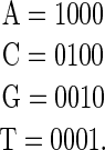 |
Sequences of any length, say L, can be made by concatenating those together in 4L-long binary strings that encode the entire sequence. This approach is used, often implicitly, whenever a weight matrix (Figure 1; also referred to as PWM or position-specific scoring matrix, PSSM) is used to score sequences for specific functions (Stormo
et al. 1982; Stormo 2000). (The matrix representation is used for convenience, to separate the elements that correspond to each position in the sequence, but the vector  is just the concatenation of the columns.) Such a weight matrix is not a unique solution as the same scores can be assigned to every sequence with different parameters, for instance, by adding any constant to every element of one column and subtracting the same constant from every element of another column. This issue is especially important when one has quantitative data, such as free energies of binding to several different sequences, and wishes to obtain the weight matrix that provides the best fit for that data (Stormo
et al. 1986; Foat
et al. 2006). Multiple linear regression provides the best-fit solution to such data but requires that there are only 3L + 1 parameters. A simple solution is to assign one reference base to be all 0's,
is just the concatenation of the columns.) Such a weight matrix is not a unique solution as the same scores can be assigned to every sequence with different parameters, for instance, by adding any constant to every element of one column and subtracting the same constant from every element of another column. This issue is especially important when one has quantitative data, such as free energies of binding to several different sequences, and wishes to obtain the weight matrix that provides the best fit for that data (Stormo
et al. 1986; Foat
et al. 2006). Multiple linear regression provides the best-fit solution to such data but requires that there are only 3L + 1 parameters. A simple solution is to assign one reference base to be all 0's,
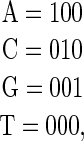 |
so that the intercept of the regression (the “+1” parameter) corresponds to the binding energy of the sequence of all T's, and the remaining parameters are the differences in binding energy to each other base (Stormo et al. 1986) (Figure 1). This is the method used by Berg and Von Hippel (1987) except that they assigned 0's to the preferred base at each position (Figure 1) so that all of the other energy parameters are positive. Other constraints on each position are also possible, such as setting the mean to 0 or setting the sum of the exponentiated parameters to 1, which corresponds to a probabilistic model. In the commonly used log-odds method the sum of exponentiated parameters times the priors for each base is set to 1 (Stormo 2000). In those methods there appear to be four parameters per position, but because of the imposed constraint only three are independent, and this complicates their use in regression methods.
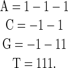
Figure 1.—

Each of these PWMs would assign the same score to every three-long sequence. (A) The parameters are all within the matrix, but the matrix is not unique; adding a constant to any column and subtracting that same constant from another column would give the same scores. (B) The T row is set to 0, and the external parameter +3 is added, which is the score for the sequence TTT. This matrix is unique given the constraint of 0's in the T row. (C) The preferred (lowest scoring) base in each column is set to 0, and the external parameter is −6, which is the score of that preferred sequence. This matrix is unique given that constraint and is the matrix obtained by the method of Berg and Von Hippel (1987).
While the 3-bit encoding provides the minimum number of parameters, it causes the vectors of different sequences to be different lengths. For many discriminant learning approaches the complexity of the problem is reduced by using the minimum number of parameters and with sequence vectors of all the same length. For example, in a quadratic programming method (Djordjevic
et al. 2003) one finds the weight vector  with minimum length that satisfies
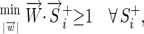 |
where  is the set of known binding sites (the “training set”). If
  is a constant, this reduces to minimizing the angle,
  , between
  and the most distant of
  because
 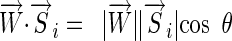 . This is equivalent to placing
  in the center of the convex hull defined by the set of
  and is the result obtained by training a support vector machine using only the positive examples (Djordjevic
et al. 2003). Other methods that learn from training examples, including both positive and negative examples, are often easiest to implement if the training vectors are all the same length. None of the commonly used encoding methods both use the minimum number of parameters and maintain equal length vectors for all sequences.
and is the result obtained by training a support vector machine using only the positive examples (Djordjevic
et al. 2003). Other methods that learn from training examples, including both positive and negative examples, are often easiest to implement if the training vectors are all the same length. None of the commonly used encoding methods both use the minimum number of parameters and maintain equal length vectors for all sequences.
Another important issue in modeling regulatory sites is the complexity of the model. The standard weight matrix method assumes that the positions of the site contribute independently (additively) to the functional activity of those sites. This is a reasonable approximation in some cases but is not true in general. One can easily extend the idea of the weight matrix to encode combinations of bases, such as dinucleotides, trinucleotides, etc. In fact one of the issues that must be addressed for any TF is the level of complexity required to adequately model its specificity (where the definition of “adequately” may vary depending on the purpose). Such higher-order encoding can use the dummy encoding described above, for example where the 1 represents a specific dinucleotide occurring at a position (Stormo et al. 1986; Zhang and Marr 1993; Lee et al. 2002; Zhou and Liu 2004). However, this approach suffers from the same limitations of either extra parameters (16 for dinucleotides where only 15 are independent) or unequal vector lengths. That idea can be extended to any higher order, but the same limitations apply. In addition, while one can compare the overall fitness of the higher-order models to that of the lower-order ones and determine which is more significant given the extra parameters, this does directly specify how well the simpler models fit the data and what is gained by each additional level of complexity. That information can be obtained by rerunning the regression multiple times using different models and comparing their fit to the data, such as by R2 values, but it is more efficient to define an overall model with parameters defining different submodels and determining the significance assigned to each parameter.
SIMPLEX ENCODING
An alternative encoding that solves all of the limitations listed above is to use simplex encoding, where sequences are encoded as the vertices of a regular 0-centered simplex. This encoding is most easily described using low-level examples and then generalizing to higher orders. For single-base models, such as the weight matrix, this corresponds to encoding each base as one of the four tetrahedral vertices of the cube centered at the origin, as has been described previously as a graphical method for displaying the distribution of bases in DNA sequences (Zhang and Zhang 1991) (Figure 2):
 |
This has the minimum number of three required parameters, all vectors are of equal length, and all vectors are equidistant from each other. For any weight vector the mean score over all possible sequences is 0, so the intercept from regression corresponds to that mean value, and each independent parameter corresponds to the difference from the mean. We refer to this as wyk encoding for the standard two-base degenerate code:
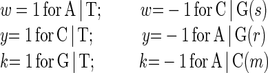 |
Figure 2.—

The tetrahedral encoding of the bases, with the origin at 0 (central dot) and each vertex of the cube being at position 1 or −1 in each dimension. The coordinates (dashed arrows) are labeled by the degenerate nucleotide code: W = (A or T), Y = (C or T), and K = (G or T). The coordinates for each base, in WYK space, are as follows: A = (1, -1, -1); C = (-1, 1, -1); G = (-1, -1, 1); T = (1, 1, 1).
HIGHER-ORDER BINDING MODELS
Higher-order models encode sequences as the vertices of a regular simplex, the equivalent of tetrahedral encoding in higher dimensions. These encodings can be constructed by the use of a Hadamard matrix,  , which is an
  matrix with each element being 1 or -1 and with the property that
 |
Hadamard matrices are conjectured to exist for all values of n that are a multiple of 4, and for  that are a power of 2 there is a very simple method of construction, shown in Figure 3. Important properties of Hadamard matrices are that all of the rows (and columns) are normal to one another (have a dot product of 0) and therefore represent a basis set for the n-dimensional space. Rows (and columns) can be exchanged without affecting any of the properties. A Hadamard matrix is said to be “normalized” if it has the top row and left column as all 1's, as in
  of Figure 3. Note that if the first column of
  is removed, we are left with the tetrahedral encoding described above (in row order T, C, A, G). By removing the first column of all 1's from any Hadamard matrix we reduce the dimensionality of the space by 1, but still have n points that are equidistant from one another, with a dot product of -1. The dot product of a row with itself is n -1. Those n points are the vertices of a regular simplex (higher-dimensional equivalent of a tetrahedron) and form the basis of the encoding for all higher levels.
Figure 3.—

Hadamard matrices. (A) Hadamard matrix for n = 1. (B) Rule for constructing Hadamard matrices for any power of 2, given H1. (C) H4 obtained by this method. This form is “normalized” with the top row and left column as all 1's.
Figure 4 shows  with the rows and columns rearranged to highlight some properties of this encoding for dinucleotides. The first column, of all 1's, corresponds to the intercept in regression, or the mean value of all the sequences, and is not used in the encoding of the sequences. This reduces the dimensionality of the space to 15 in which the 16 dinucleotide sequences are embedded. The next three columns correspond to the first base of the dinucleotide, using the 3-bit encoding described above. The next three columns are the same for the second base of the dinucleotide. The remaining nine columns are obtained as the outer product of the two bases. This construction maintains all of the desired features: it uses the minimum number of independent parameters, 15; each dinucleotide-encoding vector has the same length; and all vectors are equidistant from one another. Furthermore, regression to quantitative data determines the significance of each parameter independently and in combination they specify the fit to the data provided by each submodel. Since the number of parameters is the minimum needed, regression results in a unique solution. And since the separate mononucleotide encodings are included in the dinucleotide encoding (in positions 2–4 and 5–7 of
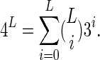
  of Figure 4), the remaining 9 dinucleotide parameters are fitting to the residuals left after the best fit by the mononucleotide positions. This means that a single regression analysis is sufficient to determine the best mononucleotide (weight matrix) model, the fraction of the total variance explained by that model, the contribution of each dinucleotide that is not explained by the mononucleotide model, and the increase in the total variance explained by including higher-order parameters. For sites of length L, for which there are 4L different sequences, one could capture all of the mononucleotide parameters plus all of the adjacent dinucleotide contributions with only
 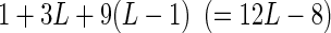 parameters. A binding site of length 10, which is fairly typical, requires only 112 parameters.
Figure 4.—

The Hadamard matrix H16 obtained as in Figure 3, except that the rows and columns have been rearranged to indicate the meaning of specific positions in the encoded sequences. The first column corresponds to the mean value of all sites and is deleted from the encoding to reduce the dimensionality to 15. The next three columns are the encoding of the first base of the dinucleotide, and the next three columns are for the second base of the dinucleotide, both based on the WYK encoding of Figure 2, as described in the text. The last nine columns are obtained as the outer product of the two base encodings. The order of those nine parameters is (w1w2, w1y2, w1k2, y1w2, y1y2, y1k2, k1w2, k1y2, k1k2) (see File S1 for an example). The column vector on the right shows the equivalence of each specific dinucleotide for each encoded string.
Figure 5 provides an example of determining the mono- and adjacent dinucleotide parameters for a three-long binding site. The binding energies for all 64 trinucleotides have been assigned in this simulated data set (see supporting information, File S1) such that an additive binding model is modified with energetic contributions from specific dinucleotides between adjacent positions 1, 2 and 2, 3, but not between positions 1, 3. A single-regression analysis provides the best-fitting weight matrix parameters, displayed as their energy contributions in the “regression logo” of Figure 5, as well as the contributions from the adjacent dinucleotides that are not explained by the additive mononucleotide parameters. At the bottom of Figure 5 is the fractional variance explained by each position, totaling 0.86 for the three independent base contributions, as well as the variance explained by the contributing dinucleotides, each contributing 0.07.
Figure 5.—

The “regression logo” (RegLogo) for the simulated data shown in File S1. The vertical axis is the energy parameter (with negative values, for the preferred bases, on top) for each mononucleotide in positions 1, 2, 3. Between them are the energy values for the adjacent dinucleotides 1, 2 and 2, 3 on the same scale. The energies for the dinucleotides are for the residual values not captured by the mononucleotide energies. So the energy for any specific three-long sequence is the sum of all the values for that sequence, including both the mononucleotide energies and the dinucleotide energies. The horizontal axis shows the variance explained by each base position and each dinucleotide. The total variance explained by a standard weight matrix is 0.86, with each dinucleotide contributing 0.07 to capture all of the variance in the data.
When encoding a functional site of length L, one can choose different levels of encoding, but will often be limited by the amount of data available. The simplest encoding would be the mononucleotide, for the standard PWM model, that requires 3L + 1 parameters (Figure 1). If one suspects there is nonadditivity (perhaps the simple model does not fit the quantitative data well), another model to test includes dinucleotides for all adjacent bases, since that is where one most expects to see the nonadditive effects (Stormo and Zhao 2007), which requires 3L + 9(L − 1) + 1 parameters, including the 9 dinucleotide parameters for the L − 1 adjacent bases in the site. Another model might include all dinucleotides, whether or not they are adjacent, which would require 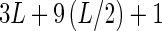 parameters, including the 9 dinucleotide parameters at the
  pairs of positions. One can add trinucleotide encoding by the same strategy of appending the 27 parameters of the three-way outer product of
  to the parameters for the three mono- and three dinucleotides. The total number of parameters for a trinucleotide encoding (including the constant term for the overall mean) is 3 × 3 + 3 × 9 + 27 + 1 = 64, which is exactly the number needed for the 64 trinucleotides. This strategy can be taken to any level, and from the expansion of the binomial coefficients we see that L-long sites, for which there are 4L different sequences, can be encoded from all of the lower-level combinations:
 |
Of course using the full encoding of all subsequence combinations requires having functional assays for all possible sequences. Current methods are making that feasible for many more transcription factors (Stormo and Zhao 2010) and in such cases one can ask why bother building a model at all, rather than simply using the functional data for each site? As described above, the model building, and especially the parameter estimation, can be useful by itself because it can provide some insight into how the sequence determines the functional activity. For example, perhaps the protein binds to sites in an essentially additive manner, in which case only the mononucleotide parameters will be significant and none of the combinatorial parameters will contribute much to the overall fit. All of the data contribute to estimating those 3L + 1 parameters, which increases their accuracy, and the fact that they explain most of the variance confirms the primarily additive mechanism of interaction. Alternatively, perhaps some of the combinatorial parameters are significant but others are not. That would also suggest how the protein recognizes the sites and distinguishes between different sequences, informing physical and structural models about the interaction. The example in Figure 5 illustrates how, in a single-regression analysis, one can get the best additive model and determine any of the nonadditive parameters and their relative importance in modeling the available data. Although shown only for the dinucleotide level in this simple example, an extended analysis can be accomplished for all higher levels, and all potentially important combinations, in a single step, limited only by the available data. Since this example used simple linear regression to obtain the parameters of the model, there is a unique optimal solution and other approaches could be used to obtain it. Typically, as in (Stormo et al. 1986; Benos et al. 2002a; Lee et al. 2002), one first obtains the best mononucleotide model and assesses its fit to the data. If a better fit is required, the regression can be rerun including high-order parameters, even fitting specifically to the residuals from the lower-order model to learn what important features were missed. The advantage of the simplex encoding strategy is that those steps are accomplished in a single run up to whatever order model is deemed potentially appropriate (and for which sufficient data exist). Furthermore, the parameters are inherently independent and represent the contrasts between different features in the data. The constant term is the overall average and each mononucleotide parameter is the difference from the average, the contrasts, for the three possible pairings of bases at each position. Higher-order parameters are the contrasts for specific combinations of bases after the lower-order effects have already been taken into account, and the independent contributions to the explained variance are obtained directly.
DISCUSSION
Binding sites for transcription factors are important components of regulatory networks. Having mathematical models to represent them allows genome searches for new regulatory targets as well as predicting the effects of genetic variations that occur within them. It can also facilitate the design of promoters and factors with novel characteristics. Current technologies expedite the high-throughput determination of the specificity of transcription factors, greatly expanding our knowledge of the factors and the regulatory networks in which they participate. But a fundamental question in modeling binding sites is the complexity of the model needed for accurate predictions. While weight matrices have dominated the field for many years, due to their increased accuracy over simple consensus sequences and small number of parameters, it is clear that in many cases they do not provide the desired accuracy. It has long been recognized that more complex models, such as including dinucleotide parameters and even higher-order models, can improve binding site predictions, but finding the optimal model has usually involved iterative assessments and comparisons. By using simplex encoding one can assess all levels of models in one test because each level is included in the model independently of the higher-order models, and the higher-order models fit the residuals from the lower-order models. As demonstrated in the example in Figure 5, a single regression analysis can obtain the best-fit weight matrix and the parameters for all of the dinucleotide residuals along with their contributions to explaining the variance.
Despite the simplicity and power of the simplex encoding scheme, some caveats remain. The examples described have used multiple linear regression to find the optimal parameters, but in some cases nonlinear regression is required to find the best model. In particular, if one obtains binding energy data for all possible sequences, many of those will likely be bound nonspecifically, where the energy is independent of the sequence (Benos et al. 2002b; Stormo and Zhao 2007). In such a case there will be significant nonadditivity, but in a somewhat trivial sense that can better accommodated by assuming two modes of binding, one specific and one nonspecific (Stormo and Zhao 2007; Zhao et al. 2009). Of course simplex encoding can be utilized for other methods of modeling binding sites besides regression, such as many different types of machine learning methods. After one has obtained an optimal model, it may be possible to further simplify it, removing parameters that contribute little or nothing to the overall fit. In the example in Figure 5, one could use dinucleotide parameters solely for the combination GC in positions 1, 2 and CA in positions 2, 3 and fit the entire data very well with only nine total parameters. But the simplex encoding allows one to obtain that conclusion efficiently without extensive exploration of many different models. It obtains all of the parameters for a given class of models, such as mononucleotide plus adjacent dinucleotides, in one step, and then subsequently one may pare the model down by eliminating parameters without significant contributions. The desired goal is to obtain a model that captures all of the important “features” of the sequence that contribute to its activity, where those may be individual bases at some positions, combinations of bases at others, and even specific characteristics of the sequences, such as complementarity between positions as for RNA structures required by RNA-binding proteins (Stormo 1988; Gorodkin et al. 1997; Sharon et al. 2008). Identifying the optimal set of features to be included in the scoring vector may require multiple assessments and comparisons, but the simplex encoding described here can still facilitate the search. The one characteristic of some binding sites that is not captured by this approach is when binding sites can be of variable length, requiring gaps when creating multiple alignments of the sites. Models allowing gaps usually require something like a hidden Markov model and are not easily encoded in vectors of fixed length, although if the variable length is quite limited they can be modeled as alternative modes of binding with separate models for each mode. Finally, it should be pointed out that Hadamard matrices exist for n = 20 so the same methods described here can be applied to protein motifs, and even to amino acid–base pair combinations, of which there are 80. Of course with so many lower-level elements the higher-order combinations explode rapidly, but it is still possible to employ the same modeling approach when sufficient data are available.
Acknowledgments
I thank Mohammed Khan and Gurmukh Sahota for writing software to convert between acgt encoding and wyk encoding and for performing the multiple regression used in Figure 5. I thank all members of the Stormo laboratory for comments on this work, especially Yue Zhao and Ryan Christensen who have tested this method on some of their data analyses. This work was supported by National Institutes of Health grant HG00249.
Supporting information is available online at http://www.genetics.org/cgi/content/full/genetics.110.126052/DC1.
References
- Benos, P. V., M. L. Bulyk and G. D. Stormo, 2002. a Additivity in protein-DNA interactions: How good an approximation is it? Nucleic Acids Res. 30 4442–4451. [DOI] [PMC free article] [PubMed] [Google Scholar]
- Benos, P. V., A. S. Lapedes and G. D. Stormo, 2002. b Is there a code for protein-DNA recognition? Probab(ilistical)ly. BioEssays 24 466–475. [DOI] [PubMed] [Google Scholar]
- Berg, O. G., and P. H. von Hippel, 1987. Selection of DNA binding sites by regulatory proteins. Statistical-mechanical theory and application to operators and promoters. J. Mol. Biol. 193 723–750. [DOI] [PubMed] [Google Scholar]
- Djordjevic, M., A. M. Sengupta and B. I. Shraiman, 2003. A biophysical approach to transcription factor binding site discovery. Genome Res. 13 2381–2390. [DOI] [PMC free article] [PubMed] [Google Scholar]
- Foat, B. C., A. V. Morozov and H. J. Bussemaker, 2006. Statistical mechanical modeling of genome-wide transcription factor occupancy data by MatrixREDUCE. Bioinformatics 22 e141–e149. [DOI] [PubMed] [Google Scholar]
- Gorodkin, J., L. J. Heyer, S. Brunak and G. D. Stormo, 1997. Displaying the information contents of structural RNA alignments: the structure logos. Comput. Appl. Biosci. 13 583–586. [DOI] [PubMed] [Google Scholar]
- Lee, M. L., M. L. Bulyk, G. A. Whitmore and G. M. Church, 2002. A statistical model for investigating binding probabilities of DNA nucleotide sequences using microarrays. Biometrics 58 981–988. [DOI] [PubMed] [Google Scholar]
- Sharon, E., S. Lubliner and E. Segal, 2008. A feature-based approach to modeling protein-DNA interactions. PLoS Comput. Biol. 4 e1000154. [DOI] [PMC free article] [PubMed] [Google Scholar]
- Stormo, G. D., 1988. Computer methods for analyzing sequence recognition of nucleic acids. Annu. Rev. Biophys. Biophys. Chem. 17 241–263. [DOI] [PubMed] [Google Scholar]
- Stormo, G. D., 2000. DNA binding sites: representation and discovery. Bioinformatics 16 16–23. [DOI] [PubMed] [Google Scholar]
- Stormo, G. D., and Y. Zhao, 2007. Putting numbers on the network connections. BioEssays 29 717–721. [DOI] [PubMed] [Google Scholar]
- Stormo, G. D., and Y. Zhao, 2010. Determining the specificity of protein-DNA interactions. Nat. Rev. Genet. 11 751–760. [DOI] [PubMed] [Google Scholar]
- Stormo, G. D., T. D. Schneider, L. Gold and A. Ehrenfeucht, 1982. Use of the ‘Perceptron’ algorithm to distinguish translational initiation sites in E. coli. Nucleic Acids Res. 10 2997–3011. [DOI] [PMC free article] [PubMed] [Google Scholar]
- Stormo, G. D., T. D. Schneider and L. Gold, 1986. Quantitative analysis of the relationship between nucleotide sequence and functional activity. Nucleic Acids Res. 14 6661–6679. [DOI] [PMC free article] [PubMed] [Google Scholar]
- Zhang, C. T., and R. Zhang, 1991. Analysis of distribution of bases in the coding sequences by a diagrammatic technique. Nucleic Acids Res. 19 6313–6317. [DOI] [PMC free article] [PubMed] [Google Scholar]
- Zhang, M. Q., and T. G. Marr, 1993. A weight array method for splicing signal analysis. Comput. Appl. Biosci. 9 499–509. [DOI] [PubMed] [Google Scholar]
- Zhao, Y., D. Granas and G. D. Stormo, 2009. Inferring binding energies from selected binding sites. PLoS Comput. Biol. 5 e1000590. [DOI] [PMC free article] [PubMed] [Google Scholar]
- Zhou, Q., and J. S. Liu, 2004. Modeling within-motif dependence for transcription factor binding site predictions. Bioinformatics 20 909–916. [DOI] [PubMed] [Google Scholar]