On Computing the Coalescence Time Density in an Isolation-With-Migration Model With Few Samples

IN a recent article, Wang and Hey (2009) consider estimation of the parameters in an isolation-with-migration (IM) model for two species. For each locus, the data X consist of two samples, and therefore the probability of the data depends only on the time to the most recent common ancestor (MRCA), and we can write the likelihood for a single locus as

where f(t|Θ) is the probability density of the coalescent time. Assuming free recombination between loci, the full likelihood is a product of each locus likelihood.

To determine the likelihood we must determine the density f(t|Θ) for coalescent of two samples in the IM model. Wang and Hey (2009) find the time to the MRCA by explicitly integrating over all possible sample paths in the system. The purpose of this letter is to demonstrate that the time to the MRCA is easy to compute from a matrix exponential. Furthermore, the matrix exponential framework has the advantage that it generalizes to more than two samples. We describe the IM model, briefly describe the solution to computing the coalescence time density from Wang and Hey (2009), and finally present an approach that computes the density through matrix exponentials.

The description of the model is taken from Wang and Hey (2009) and formulates the IM model as a continuous time Markov chain. Before time T and for two samples the system is in one of the following five states: S₁₁, both genes are in population 1; S₂₂, both genes are in population 2; S₁₂, one gene is in population 1 and the other is in population 2; S₁, the genes have coalesced and the single gene is in population 1; and S₂, the genes have coalesced and the single gene is in population 2. The rates between the states can be described by the instantaneous rate matrix Q given by

(1)

where the diagonals are such that each row sums to zero. After time T, the system only has two states: S_AA corresponding to two genes in the ancestral population and S_A corresponding to one single gene in the ancestral population. The rate of going from state S_AA to state S_A is 2/θ_A. The model parameters are thus Θ = (θ₁, θ₂, θ_A, m₁, m₂, T), where θ₁, θ₂, and θ_A are the scaled population sizes, m₁ and m₂ are the migration rates and T is the speciation time. We refer to Wang and Hey (2009, Figure 1) for an illustration of the model and for more details on the model parameters.

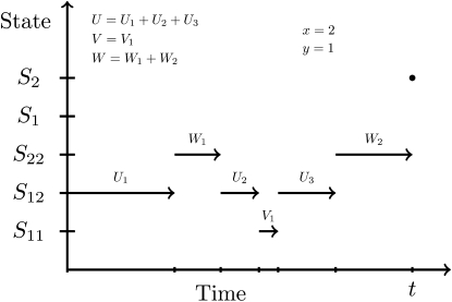
Figure 1.—

Illustration of a sample path with coalescent in population 2 at time t.

Now consider the sample path z = {z(s) : 0 ≤ s ≤ t } shown in Figure 1, where the coalescent happens at time t < T and in population 2. The density for this sample path is given by

where x and y are the number of transitions to the states S₁₂ and S₁₁, respectively. The number of transitions from S₁₁ to S₁₂ and from S₁₂ to S₁₁ is therefore y and, since the starting state is S₁₂, the number of transitions from S₁₂ to S₂₂ and S₂₂ to S₁₂ is x − y + 1 and x − y. The variables U, V, and W are the total amount of time spent in the states S₁₂, S₁₁, and S₂₂, respectively.

To determine the density f₂(t|Θ) for coalescent in population 2 at time t < T, Wang and Hey (2009) explicitly integrate all possible sample paths that find a MRCA at time t. The integration is performed by first integrating all sample paths that share the same values for the five variables (x, y, U, V, W); this density is termed p(x, y, U, V, W |Θ). Second, this expression is summed over variables (x, y) and integrated over variables (U, V, W) with the constraint U +V +W = t:

The inner summation becomes a Bessel I_α(x) function and the two-dimensional planar integration is handled numerically.

It is possible, however, to take immediate advantage of the continuous time Markov chain representation (1) and to solve the system of ordinary differential equations analytically. The two samples are either from the same species (corresponding to the starting state being S₁₁ or S₂₂) or the two samples are from each of the species (in which case the starting state is S₁₂). Starting in state a, the density for coalescent in population 1, for t < T, is given by

(2)

where e^A is the matrix exponential and (e^A)_jk is entry (j, k) in e^A. Calculating matrix exponentials has a very long history (e.g., Moler and Van Loan 2003), and implementations are available in most standard computer languages. The density for coalescent in population 2 at time t < T is

(3)

and the total density for a coalescent at time t < T is

(4)

Similarly, the density for coalescent in the ancestral population at time t > T is

(5)

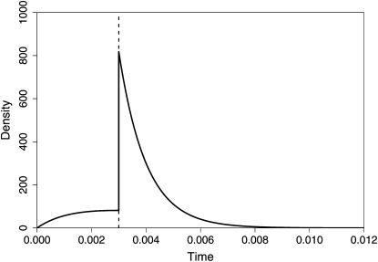
In Figure 2 we illustrate the coalescent density in the two species IM model. We use the same parameters as in the simulation study in Wang and Hey (2009, Table 6): θ₁ = 0.005, θ₂ = 0.003, θ_A = 0.002, m₁ = 50, m₂ = 100, and T = 0.003 (the vertical line).

Figure 2.—

Illustration of the density (4) and (5) for coalescent in the two species isolation with migration model.

Multiple analytical approaches for computing the coalescence time density can be found in the literature. Variations of the IM model have been analyzed using Laplace transforms in, e.g., Latter (1973), Takahata (1995), and Wilkinson-Herbots (1998). Their results can also be derived using matrix exponentiation. In Wakeley (1996), a spectral decomposition was used to obtain a continuous-time approximation to a discrete time model. Generalizations of the IM model dealing with two loci with recombination between loci are analyzed using expressions for continuous time Markov chains in Slatkin and Pollack (2006) and Simonsen and Churchill (1997).

We finally emphasize that the matrix exponential framework described above generalizes to more than two samples and more than two populations. For any coalescence system that can be expressed as a finite-state homogeneous continuous time Markov chain, we can compute the density of coalescence times using matrix exponentiation. Expressing a coalescence process as such a system is straightforward although a major complication is an explosion in the number of states when the number of samples and populations increase.

If the Markov chain is not homogeneous, that is, the rate matrix Q depends on the time parameter t, simple matrix exponentiation is no longer a solution to the coupled set of differential equations. The model of Innan and Watanabe (2006), for instance, consists of the same set of states and almost the same rate matrix, but has the migration rates depend linearly on the time variable t. For this system, the approach described above cannot be applied.

References

- Innan, H., and H. Watanabe, 2006. The effect of gene flow on the coalescent time in the human–chimpanzee ancestral population. Mol. Biol. Evol. 23 1040–1047. [DOI] [PubMed] [Google Scholar]
- Latter, B. D. H., 1973. The island model of population differentiation: a general solution. Genetics 73 147–157. [DOI] [PMC free article] [PubMed] [Google Scholar]
- Moler, C., and C. Van Loan, 2003. Nineteen dubious ways to compute the exponential of a matrix, twenty-five years later. SIAM Rev. 45 3–49. [Google Scholar]
- Simonsen, K. L., and G. A. Churchill, 1997. A Markov chain model of coalescence with recombination. Theor. Popul. Biol. 52 43–59. [DOI] [PubMed] [Google Scholar]
- Slatkin, M., and J. L. Pollack, 2006. The concordance of gene trees and species trees at two linked loci. Genetics 172 1979–1984. [DOI] [PMC free article] [PubMed] [Google Scholar]
- Takahata, J., 1995. A genetic perspective on the origin and history of humans. Annu. Rev. Ecol. Syst. 26 343–372. [Google Scholar]
- Wakeley, J., 1996. Pairwise differences under a general model of population subdivision. Genetics 75 81–89. [Google Scholar]
- Wang, Y., and J. Hey, 2009. Estimating divergence parameters with small samples from a large number of loci. Genetics 184 363–379. [DOI] [PMC free article] [PubMed] [Google Scholar]
- Wilkinson-Herbots, H. M., 1998. Genealogy and subpopulation differentiation under various models of population structure. J. Math. Biol. 37 535–585. [Google Scholar]