Torsional Kinematic Model for Concentric Tube Robots

Abstract

A recent approach to steerable needle design is based on combining pre-curved tubes concentrically. By rotating and extending the tubes with respect to each other, the position and orientation of the needle tip, as well as the shape of the inserted length, can be controlled. Prior models neglected torsional twisting in the curved portions of the tubes. This paper presents a mechanics model that includes torsion, applies to any number of tubes and allows curvature and stiffness to vary with arc length. While the general model is comprised of differential equations, an analytic solution is given for two tubes of constant curvature. This solution enables analytic prediction of “snap through” instability based on a single dimensionless parameter. Simulation and experiments are used to illustrate the results.

I. INTRODUCTION

THE challenge of most existing needle-based medical procedures is the safe and accurate navigation of the needle through tissue to the desired target. This topic has received considerable recent attention from the robotics community with efforts focused on two topics, path planning and image-based feedback control, to accommodate needle and tissue deformation in reaching a target.

Once the target is reached, the subsequent step is very simple and usually consists of using the needle’s lumen to either deliver drugs or radioactive seeds or to capture a biopsy sample. Many new and exciting needle-based interventions could be developed, however, if the needle’s shape could be actively controlled along its entire length. An important class of applications for such a device would be to enter a body lumen by steering through tissue or through a body orifice. Once inside the lumen, the proximal portion can remain relatively fixed while the distal portion manipulates tools within the lumen to perform minimally invasive surgery.

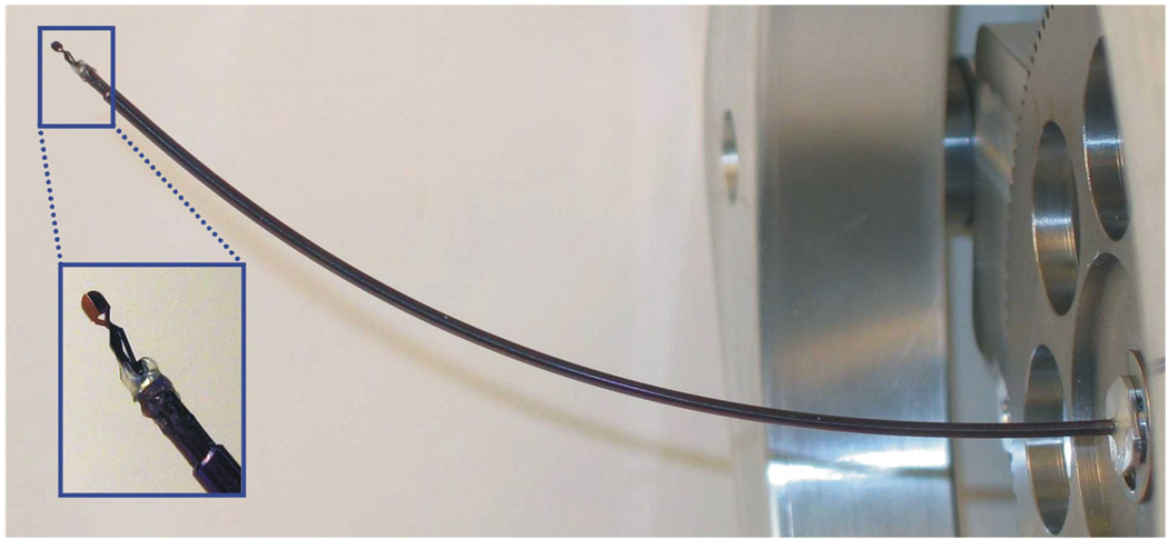
A promising technology for constructing such steerable needle robots is based on the concentric combination of precurved elastic tubes [6]–[12]. The shape of the robotic needle as well as its tip position and orientation can be actively controlled by relative rotation and translation of the tubes at their proximal end. The lumen of the tubes can house tubes and wires for control of tip-mounted tools. A simple example is shown in Fig. 1 in which actuated linear motion of a wire inside the robot opens and closes the tip-mounted forceps.

Fig. 1.

Concentric tube robot with 1 mm diameter tip-mounted forceps.

The kinematic modeling for real-time control of these robots is challenging in comparison to that of traditional robots whose links are relatively rigid and whose joints are discrete. The forward kinematics can be cast as a 3D beam bending problem in which the kinematic input variables (tube rotations and displacements at the proximal end) enter the problem as a subset of the boundary conditions. The remaining boundary conditions are comprised of point forces and torques applied to the distal ends of the tubes.

Contact along the robot’s length (e.g., with tissue) generates additional distributed and point loads. Thus, it can be anticipated that the forward kinematics can be expressed as a two-point boundary value problem involving a differential equation with respect to arc length along the common center line of the tubes. Phenomena which may be included in the model are bending, torsion, friction, shear, axial elongation and nonlinear constitutive behavior.

Real-time control necessitates balancing accuracy of the model with efficiency of its computation. Thus, efforts to date have modeled curved portions of the tubes as piecewise constant curvature and experiencing pure bending [6]–[12]. This choice results in an algebraic expression for curvature of the combined tubes which can be analytically integrated to yield position and orientation of the robot’s tip. Models of this type have been demonstrated to provide reasonable performance in combination with real-time sensing of the tip frame (teleoperation in [9], image servoing in [12]). It remains an open question, however, as to what the most appropriate kinematic control model may be and what phenomena it should include. Furthermore, certain phenomena may be important to model during robot design, but may not need be included in an on-line model.

Toward answering these questions, this paper presents a mechanics model that incorporates bending and torsion for any number of tubes whose stiffness and initial curvature can be arbitrary functions of arc length. The paper is arranged as follows. The next section reviews related work. Section III presents the model. Section IV provides an analytic solution of the model for two tubes of constant curvature and describes when such tubes can experience a “snap through” instability. Section V presents validation experiments and the final section presents conclusions.

II. RELATED WORK

When curved tubes are inserted inside each other, their common axis must conform to a mutual resultant curvature. By performing relative translations and rotations of the tubes, both the curvature as well as the overall length of the robot can be varied. The first robots of this type composed of two tubes were presented in [3],[4],[5]. Robots composed from three or more tubes were first proposed in [6],[7].

In [6], a forward kinematic model was derived for an arbitrary number of tubes of piecewise constant curvature. The model assumes that the tubes are torsionally rigid, frictionless, linear elastic and that each tube experiences piecewise constant bending moments along its length. The latter assumption implies that shear deformation of the cross section as well as axial elongation are also negligible. In addition, it is assumed that no external loads are applied. Using this model, tubes of piecewise constant curvature combine to form robots of piecewise constant curvature whose shape can be computed using an algebraic equation. A similar equation for two constant-curvature tubes was conjectured, but not proven in [7].

While it was shown in [8] that closed form inverse kinematic solutions can be derived for simple robot designs, they are difficult to obtain for more general designs. A Jacobian-based inverse kinematic solution for an arbitrary number of piecewise constant curvature tubes using the algebraic curvature model was formulated and demonstrated in simulation in [8] and experimentally on a 3-tube teleoperated system in [9].

Experimental evaluation of the curvature model on pairs of constant curvature tubes did not provide an accurate fit to the data [6],[9]. It was observed, however, that the combined tube shape closely matched constant curvature arcs. Thus, an accurate kinematic model could be obtained using a truncated Fourier series to represent curvature and plane angle as periodic functions of relative tube rotation angle [6]. Alternately, these functions could be implemented efficiently using a table driven model and this approach was implemented on a teleoperated 3-tube robot operated at 1 kHz in [9].

Empirical input-output maps such as these are well suited to real-time control applications and have the benefit of accounting for all unmodeled phenomena including torsion, friction and nonlinear elasticity. Since they are not true representations of the underlying physics, however, they cannot provide insights for robot design (e.g, how to eliminate “snap through” instabilities). Furthermore, if physics-based models amenable to real-time control could be developed, they would likely require less complicated online calibration and produce smaller errors than would a functionally approximate model.

To this end, an energy model that included torsional windup in the straight transmission lengths of the tubes was proposed in [7] and numerical energy minimization was suggested as a means of solving for transmission twist. This model, which assumes that the curved portions of the tubes are torsionally rigid, was used to investigate solution multiplicity and stability for a pair of curved elements in [11] and employed for visual servoing of a two-tube robot in [12].

Torsional twist occurs along the entire length of the tubes. The relative contribution to the overall robot shape of twist in the straight transmission sections versus the curved sections will depend on both the design of the drive system and the application-specific robot design. Thus, it is desirable to develop a model that includes twist in both the curved and straight sections of the tubes.

III. MECHANICS MODEL INCORPORATING TORSION

Here, we consider tubes of arbitrary initial curvature and incorporate the effect of torsion due to bending along the entire length the tubes. We show that the model can be derived either from the special Cosserat rod model or using the calculus of variations. The resulting model is a differential equation which must be integrated along the length of the tubes to determine twist angle, and thus curvature, as a function of arc length. To define coordinates and introduce terminology, we first briefly review the torsionally rigid model of [6].

A. Torsionally Rigid Algebraic Curvature Model

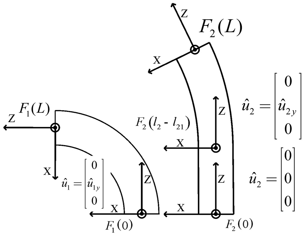
The tubes are labeled with subscript indices, i = 1, 2,…,n , where 1 is the outermost tube and n is the innermost tube. As shown in Fig. 2, material coordinate frames for each cross section can be defined as a function of arc length s along tube i by defining a single frame at the proximal end, F_i(0), such that its z axis is tangent to the tube’s centerline. Under the assumption that the tubes do not possess initial material torsion, the frame, F_i(s), is obtained by sliding F_i(0) along the tube centerline without rotation about its z axis. As the tubes bend and rotate, the frames move with their cross sections. Assuming torsional rigidity, any relative rotation between the tubes will be constant along their entire length. We can also define a reference frame, F₀(s), which does not rotate about its z axis. When needed for clarity, superscripts will be used to indicate the coordinate frame of vectors and transforms.

Fig. 2.

Tube coordinate frames and initial curvatures.

As the i^th tube’s coordinate frame F_i(s) slides down its centerline, it experiences a body-frame angular rate of change per unit arc length given by

$$u_i^{F_i(s)}(s)={\left[u_{\mathit{\text{ix}}}(s)u_{\mathit{\text{iy}}}(s)u_{\mathit{\text{iz}}}(s)\right]}^T$$ (1)

in which (u_ix,u_iy) are the components of curvature due to bending and u_iz = 0 is the curvature component due to torsion. A circumflex on a curvature component is used to designate the initial undeformed curvature of a tube. In the examples of Fig. 2, the tubes have nonzero y components of curvature.

The algebraic curvature model can be derived by combining three equations – a constitutive model relating bending moments to changes in curvature of individual tubes, the equilibrium of bending moments for the assembled tubes and a compatibility equation relating the individual curvatures of the assembled tubes.

When the tubes are assembled concentrically, the bending moment vector at any point along tube i is given by

$$m_i^{F_i(s)}(s)=K_i\left(u_i^{F_i(s)}(s)-{\widehat{u}}_i^{F_i(s)}(s)\right)$$ (2)

in which $m_i^{F_i(s)}(s)$ is the moment vector, $u_i^{F_i(s)}(s)\text{ and }{\widehat{u}}_i^{F_i(s)}(s)$ are the resultant and initial angular frame rates and K_i is the frame-invariant stiffness tensor for a tube given by

$$K_i=\left[\begin{array}{ccc}\hfill k_{\mathit{\text{ix}}}\hfill & \hfill 0\hfill & \hfill 0\hfill \\ \hfill 0\hfill & \hfill k_{\mathit{\text{iy}}}\hfill & \hfill 0\hfill \\ \hfill 0\hfill & \hfill 0\hfill & \hfill k_{\mathit{\text{iz}}}\hfill \end{array}\right]=\left[\begin{array}{ccc}\hfill E_i{I}_i\hfill & \hfill 0\hfill & \hfill 0\hfill \\ \hfill 0\hfill & \hfill E_i{I}_i\hfill & \hfill 0\hfill \\ \hfill 0\hfill & \hfill 0\hfill & \hfill J_i{G}_i\hfill \end{array}\right]$$ (3)

in which E_i is the modulus of elasticity, I_i is the area moment of inertia, J_i is the polar moment of inertia and G_i is the shear modulus.

While (2) applies on a point-wise basis, the pure bending assumption permits it to be applied to sections of the robot in which each tube has constant initial curvature. The moment equilibrium equation can be applied to each of these sections by transforming (2) for each tube to a single frame such as F₀(s). Defining θ_i as the z axis rotation angle from frame F₀(s) to frame F_i(s), the curvature vectors transform as

$$u_i^{F_0(s)}=R_z(\theta )u_i^{F_i(s)}.$$ (4)

in which R_z(θ_i) is a rotation matrix. The moment equilibrium equation for the concentric tubes is

$${\displaystyle \sum _{i=1}^n{m}_i^{F_0(s)}}=0.$$ (5)

Since all tubes must conform to the same final curvature, the compatibility equation is given by

$$u_1^{F_0(s)}=u_2^{F_0(s)}=\cdots =u_n^{F_0(s)}$$ (6)

Combining (2)–(6) yields an expression for the resultant angular frame rate for a section of needle length comprised of n overlapping tubes of constant curvature,

$$u_i^{F_0(s)}={\left({\displaystyle \sum _{i=1}^n{K}_i}\right)}^{-1}{\displaystyle \sum _{i=1}^n{K}_i}{\widehat{u}}_i^{F_0(s)}.$$ (7)

Assuming torsional rigidity and piecewise constant curvature of the individual tubes, this expression is constant, $u_i^{F_0(s)}(s)={\left[u_{\mathit{\text{ix}}}{u}_{\mathit{\text{iy}}}0\right]}^T$ , for each section of the robot in which each tube has constant initial curvature.

B. Torsionally Compliant Model for Two Tubes Derived Using Special Cosserat Rod Equilibrium Model

Instead of writing equilibrium and compatibility equations for each constant curvature section of the robot as was done in (5) and (6), we must now write them on a point-wise basis as a function of arc length. For clarity of presentation, the model is derived here for two tubes of constant curvature. It is convenient to define the relative twist angle α(s) between tubes as a function of arc length,

$$\alpha (s)={\theta }_2(s)-{\theta }_1(s)$$ (8)

where θ_i(s) is the angular displacement of the ith tube at arc length s. Equilibrium of moments must hold on every cross section and can be written in the body frame of tube 1 as

$$m_1^{F_1(s)}(s)=-R_z(\alpha (s))m_2^{F_2(s)}.$$ (9)

With torsional twisting, the compatibility equation enforcing the coincidence of tube centerlines becomes

$$u_1^{F_1(s)}(s)=R_z(\alpha )u_2^{F_2(s)}(s)-\dot{\alpha }(s)e_z$$ (10)

in which e_z = [0, 0, 1]^T and α̇ = dα / ds. This equation ensures that the tubes experience the same curvature in the plane of the cross section, but allows different rates of torsional twist.

In the subsequent presentation, all variables are defined in the body frames of the tubes and we omit reference to the frames. Thus, $u_2^{F_2(s)}(s)$ is written as u₂(s).

Combining the moment equilibrium equation of (9) with the constitutive model (2) and the compatibility equation (10) leads to an expression for the curvature of tube 2. Assuming circular cross sections, R_z(α) and K_i commute yielding

$$u_2={(K_1+K_2)}^{-1}(R_z^T(\alpha )K_1{\widehat{u}}_1+K_2{\widehat{u}}_2+\dot{\alpha }{K}_1{e}_z)$$ (11)

The x and y components of this equation mirror those of the torsionally rigid case and provide explicit algebraic equations for curvature as a function of initial curvature and twist angle α.

$$u_2{|}_{x,y}={(K_1+K_2)}_{x,y}^{-1}{(R_z^T(\alpha )K_1{\widehat{u}}_1+K_2{\widehat{u}}_2)}_{x,y}$$ (12)

$$u_1{|}_{x,y}={(R_z(\alpha )u_2)}_{x,y}$$ (13)

The z component of (11) provides an expression for twist angle rate, α̇.

$$\dot{\alpha }=(1+k_{2z}/k_{1z})u_{2z}$$ (14)

Here we have used the fact that initial curvature does not include torsional twist. To solve this expression, we need to be able to evaluate u_2z.

We can obtain such an expression from the equilibrium equation of the special Cosserat rod model [2]. Setting time dependent terms to zero, the body-frame equilibrium equations for a curved rod undergoing distributed loading of τ ∈ ℝ³ torque per unit length and f ∈ ℝ³ force per unit length are given by

$$\left[\begin{array}{c}\hfill \dot{m}\hfill \\ \hfill \dot{n}\hfill \end{array}\right]=\left[\begin{array}{c}\hfill \tau \hfill \\ \hfill f\hfill \end{array}\right]-\left[\begin{array}{cc}\hfill [u]\hfill & \hfill [v]\hfill \\ \hfill 0\hfill & \hfill [u]\hfill \end{array}\right]\left[\begin{array}{c}\hfill m\hfill \\ \hfill n\hfill \end{array}\right]$$ (15)

Here, derivatives are with respect to arc length along the rod, s, and m, n ∈ ℝ³ are the bending moment and shear force vectors acting on the rod’s cross section. The vectors u, v ∈ ℝ³ are the angular and linear strain rates per unit arc length and square brackets indicate the skew symmetric matrix form. If one imagines sliding along a curved rod, these vectors can be interpreted as linear and angular velocities (twist velocities) with arc length corresponding to time. Wrenches applied at either end of the rod enter the equations as boundary conditions.

This equation can be used to predict the shape and forces exerted when two or more precurved tubes are combined concentrically. Since we anticipate that bending and twisting will be the dominant forms of deformation of the tubes, we continue to assume that shear strain and axial strain are negligible. In (15), this results in v^T = [0, 0, 1]. Furthermore, we assume that contact between the tubes is frictionless and that tubes can only exert distributed reaction forces, but not torques, on each other. As with the torsionally rigid model, we assume that concentrated moments are generated over negligibly short lengths at the ends of the tubes in order to satisfy compatibility (12),(13). These moments are treated as boundary conditions in (15).

Since tube interaction is limited to distributed forces, τ = 0 in (15) and, for each tube, it reduces to

$${\dot{m}}_i=-[u_i]m_i-[v_i]n_i$$ (16)

To eliminate moments from these equations, we can use the constitutive model for moments (2) and its derivative with respect to arc length,

$${\dot{m}}_i=K_i{\dot{u}}_i$$ (17)

In the derivative, we have taken K_i and û_i to be independent of s for simplicity, but this is not necessary. Equation (16) can now be rewritten in terms of curvature

$${\dot{u}}_i=-K_i^{-1}[u_i]K_i(u_i-{\widehat{u}}_i)-K_i^{-1}[v_i]n_i$$ (18)

Recalling v_i = [0, 0, 1]^T and assuming equal bending stiffness in the x and y directions, k_ix = k_iy, the z component of (18) provides an expression for the derivative of torsional twist rate as a function of bending curvature,

$${\dot{u}}_{2z}=(k_{2x}/k_{2z})(u_{2x}{\widehat{u}}_{2y}-u_{2y}{\widehat{u}}_{2x})$$ (19)

This simple equation indicates that the derivative of twist rate is given by the cross product between actual and initial bending curvature multiplied by the ratio of bending and torsional stiffness. For tubes, this ratio is given by

$$k_{\mathit{\text{ix}}}/k_{\mathit{\text{iz}}}=G_i{J}_i/E_i{I}_i=1+\nu$$ (20)

in which ν is Poisson’s ratio. By equilibrium of torsional moments, we need only integrate for u_1z or u_2z since

$$u_{1z}=-(k_{2z}/k_{1z})u_{2z}$$ (21)

Equations (12),(14),(19) comprise the set of equations that must be solved to compute 3D curvature along the length of the tubes. Equations (14) and (19) are two first-order differential equations that can be equivalently described by a second order equation in α. If we assume that the initial cross sectional curvature of both tubes is in the same direction (e.g., both in x direction or both in y direction) when α = 0 then the three equations reduce to the following simple expression for initial curvature magnitudes ‖û₁‖ and ‖û₂‖.

$$\ddot{\alpha }(s)=(1+\nu )\Vert {\widehat{u}}_1\Vert \Vert {\widehat{u}}_2\Vert \text{sin }\alpha (s)$$ (22)

This equation indicates that the second derivative of twist angle has a simple dependence on Poission’s ratio and initial curvatures of the tubes.

Two boundary conditions are needed for the two state variables, (α, α̇) or (α,u_2z). Since the tube angles at the proximal end, θ_i(0), are the kinematic input variables,

$$\alpha (0)={\theta }_2(0)-{\theta }_1(0).$$ (23)

In addition, the torsional bending moment at the distal end of each tube is zero,

$$m_{2z}(L)=k_{2z}(u_{2z}(L)-{\widehat{u}}_{2z}(L))=k_{2z}{u}_{2z}(L)=0$$ (24)

This yields a second boundary condition

$$\dot{\alpha }(L)=u_{2z}(L)=0$$ (25)

This is a two-point boundary value problem. As we will show in a subsequent section, (22) can be integrated analytically. First, we show that it can be derived from energy considerations without employing the special Cosserat rod model.

C. Torsionally Compliant Model for Two Tubes Derived Using Calculus of Variations

The equation describing torsional twisting of the tubes can also be derived as the solution that minimizes strain energy in the tubes. An expression for total strain energy U due to bending and torsion is given by

$$U={\displaystyle \sum _{i=1}^2\frac{1}{2}{\displaystyle \underset{0}{\overset{L}{\int }}\left(\frac{{\Vert m_i{|}_{x,y}\Vert }^2}{E_i{I}_i}+\frac{m_{\mathit{\text{iz}}}^2}{G_i{J}_i}\right)}\mathit{\text{ds}}}$$ (26)

in which the first term accounts for bending and the second for torsion. Since strain energy will be invariant under rigid body motion of the tube pair, we anticipate that it can be written as a function of the relative twist angle α(s).

The constitutive model (2) provides expressions for bending moment m_i|_x,y and torque m_iz,

$$m_i{|}_{x,y}=E_i{I}_i(u_i-{\widehat{u}}_i){|}_{x,y}$$ (27)

$$m_{\mathit{\text{iz}}}=G_i{J}_i{u}_{\mathit{\text{iz}}}$$ (28)

Substituting these into (26) results in

$$U={\displaystyle \sum _{i=1}^2\frac{1}{2}{\displaystyle \underset{0}{\overset{L}{\int }}\left(E_i{I}_i{\Vert (u_i-{\widehat{u}}_i){|}_{x,y}\Vert }^2+G_i{J}_i{u}_{\mathit{\text{iz}}}^2\right)\mathit{\text{ds}}}}$$ (29)

Equations (12) and (13) can be used to compute the norm in the first term yielding

$${\Vert (u_1-{\widehat{u}}_1){|}_{x,y}\Vert }^2=\frac{E_2{I}_2}{{(E_1{I}_1+E_2{I}_2)}^2}{\Vert {\widehat{u}}_2-R_z^T(\alpha ){\widehat{u}}_1\Vert }^2$$ (30)

$${\Vert (u_2-{\widehat{u}}_2){|}_{x,y}\Vert }^2=\frac{E_1{I}_1}{{(E_1{I}_1+E_2{I}_2)}^2}{\Vert {\widehat{u}}_1-R_z(\alpha ){\widehat{u}}_2\Vert }^2$$ (31)

Equation (14) can be used to express u_2z in terms of α̇.

$$u_{2z}=\left(\frac{G_1{J}_1}{G_1{J}_1+G_2{J}_2}\right)\dot{\alpha }$$ (32)

Moment equilibrium (9) and the constitutive model (2) provide an expression for u_1z,

$$u_{1z}=\left(\frac{-G_2{J}_2}{G_1{J}_1}\right)u_{2z}=\left(\frac{-G_2{J}_2}{G_1{J}_1+G_2{J}_2}\right)\dot{\alpha }$$ (33)

Using (30)–(33), total strain energy (29) can be written as a function of the tube parameters and relative twist angle, α(s),

$$U=\frac{1}{2}{\displaystyle \underset{0}{\overset{L}{\int }}\left(\frac{(E_1{I}_1)(E_2{I}_2)}{E_1{I}_1+E_2{I}_2}{\Vert ({\widehat{u}}_1-R{\widehat{u}}_2){|}_{x,y}\Vert }^2+\frac{(G_1{J}_1)(G_2{J}_2)}{G_1{J}_1+G_2{J}_2}{\dot{\alpha }}^2\right)}\mathit{\text{ds}}$$ (34)

The Euler Lagrange equation provides necessary conditions for the function α(s) that minimizes (34) and is given by

$$\frac{d}{\mathit{\text{ds}}}\left(\frac{\partial U}{\partial \dot{\alpha }}\right)=\frac{\partial U}{\partial \alpha }$$ (35)

Applying (35) to (34) results in

$$\ddot{\alpha }(s)=(1+\nu )\Vert {\widehat{u}}_1\Vert \Vert {\widehat{u}}_2\Vert \text{sin}\alpha (s)$$ (36)

which is the same as (22).

The Legendre condition provides a second-order necessary condition for (36) to be a minimum energy solution and is given by

$$\frac{{\partial }^{2}U}{\partial \dot{\alpha }\partial \dot{\alpha }}\ge 0,\forall s\in [0,L]$$ (37)

which is clearly satisfied by (34).

In robotic applications, the proximal ends of the tubes are mounted in motor-controlled bearings and so α(0) is under direct control. While tube length L is fixed, the twist angle at the distal end α(L) is free in the minimization. This leads to the natural boundary condition for the minimizing solution α^*

$$\frac{\partial U}{\partial \dot{\alpha }}\left({\alpha }^{*},{\dot{\alpha }}^{*},L\right)=0$$ (38)

from which we recover the zero-torque boundary condition (25).

D. Torsional Model for an Arbitrary Number of Tubes

The equations above can easily be extended to include any number of tubes of arbitrary stiffness and initial curvature as is now shown. Consider the case of n concentric tubes numbered from outer tube to inner tube. To write equations in the coordinate frame of the outer tube 1, we define the relative twist angles as

$${\alpha }_i(s)={\theta }_i(s)-{\theta }_1(s),i=2,\dots ,n$$ (39)

where θ_i(s) is the angular displacement of the ith tube at arc length s. Equilibrium of moments and forces must hold on every cross section and can be written as

$$\left[\begin{array}{c}\hfill m_1(s)\hfill \\ \hfill n_1(s)\hfill \end{array}\right]+\left[\begin{array}{cc}\hfill R_z({\alpha }_2(s))\hfill & \hfill 0\hfill \\ \hfill 0\hfill & \hfill R_z({\alpha }_2(s))\hfill \end{array}\right]\left[\begin{array}{c}\hfill m_2(s)\hfill \\ \hfill n_2(s)\hfill \end{array}\right]+\cdots +\left[\begin{array}{cc}\hfill R_z({\alpha }_n(s))\hfill & \hfill 0\hfill \\ \hfill 0\hfill & \hfill R_z({\alpha }_n(s))\hfill \end{array}\right]\left[\begin{array}{c}\hfill m_n(s)\hfill \\ \hfill n_n(s)\hfill \end{array}\right]=0$$ (40)

The compatibility equation enforcing the coincidence of tube centerlines becomes

$$\begin{array}{cc}{u}_1(s)\hfill & =R_z({\alpha }_2)u_2(s)-{\dot{\alpha }}_2(s)e_z\hfill \\ \hfill & =\cdots \hfill \\ \hfill & =R_z({\alpha }_n)u_n(s)-{\dot{\alpha }}_n(s)e_z\hfill \end{array}$$ (41)

Combining the moment equation of (40), the compatibility equation (41) and constitutive model (2) results in

$$u_1={\left(K_1+R_2{K}_2{R}_2^T+\cdots +R_n{K}_n{R}_n^T\right)}^{-1}·\left((K_1{\widehat{u}}_1+R_2{K}_2{\widehat{u}}_2+\cdots +R_n{K}_n{\widehat{u}}_n)-\left({\dot{\alpha }}_2{R}_2{K}_2{R}_2^T+\cdots +{\dot{\alpha }}_n{R}_n{K}_n{R}_n^T\right)e_z\right)$$ (42)

where we have used the shorthand notation R_i = R_z (α_i).

This can be simplified when k_ix = k_iy, e.g., circular cross sections of homogeneous material, using $K_i=R_i{K}_i{R}_i^T$ to obtain

$$u_1={(K_1+K_2+\cdots +K_n)}^{-1}·((K_1{\widehat{u}}_1+R_2{K}_2{\widehat{u}}_2+\cdots +R_n{K}_n{\widehat{u}}_n)-({\dot{\alpha }}_2{K}_2+\cdots +{\dot{\alpha }}_n{K}_n)e_z)$$ (43)

We can also write the more general equation for curvature of the i^th tube as

$${\displaystyle \sum _{j=1}^n\left(R_j{K}_j{R}_j^T\right)R_i{u}_i}={\displaystyle \sum _{j=1}^n{R}_j{K}_j{\widehat{u}}_j+}{\displaystyle \sum _{j=1}^n{R}_j{K}_j{R}_j^T}\left({\dot{\alpha }}_i-{\dot{\alpha }}_j\right)e_z$$ (44)

In (44), note that R₁ is the identity matrix and α̇₁ = 0.

Again using $K_i=R_i{K}_i{R}_i^T$ , we can solve for u_i as

$$u_i={\left({\displaystyle \sum _{j=1}^n{K}_j}\right)}^{-1}{R}_i^T\left({\displaystyle \sum _{j=1}^n{R}_j{K}_j{\widehat{u}}_j+}{\displaystyle \sum _{j=1}^n{K}_j({\dot{\alpha }}_i-{\dot{\alpha }}_j)e_z}\right)$$ (45)

The x and y components of curvature can be obtained from (45) as

$$u_i{|}_{x,y}={\left({\left({\displaystyle \sum _{j=1}^n{K}_j}\right)}^{-1}{R}_i^T\left({\displaystyle \sum _{j=1}^n{R}_j{K}_j{\widehat{u}}_j}\right)\right)|}_{x,y},i=1,\dots ,n$$ (46)

The rates of relative twist angles can be computed from (41) as

$${\dot{\alpha }}_i=u_{\mathit{\text{iz}}}-u_{1z},i=2,\dots ,n$$ (47)

To obtain an expression for u_iz we combine the constitutive model (2) and its derivative with

$${\dot{m}}_i=-[u_i]m_i-[v_i]n_i$$ (48)

to arrive at

$${\dot{u}}_i={\dot{\widehat{u}}}_i-K_i^{-1}\left([u_i]K_i(u_i-{\widehat{u}}_i+[v_i]n_i\right)$$ (49)

Using v_i = [0, 0, 1]^T and assuming equal bending stiffness the x and y directions, k_ix = k_iy, the z component yields the desired expression as

$${\dot{u}}_{\mathit{\text{iz}}}={\dot{\widehat{u}}}_{\mathit{\text{iz}}}+(k_{\mathit{\text{ix}}}/k_{\mathit{\text{iz}}})(u_{\mathit{\text{ix}}}{\widehat{u}}_{\mathit{\text{iy}}}-u_{\mathit{\text{iy}}}{\widehat{u}}_{\mathit{\text{ix}}})$$ (50)

While (50) holds for i = 1,…,n, we need only evaluate and integrate it for i = 2,…,n. Equilibrium of moments (40) together with the constitutive model (2) enable us to solve for u_1z as

$$u_{1z}=(-1/k_{1z})(k_{2z}{u}_{2z}+\dots +k_{\mathit{\text{nz}}}{u}_{\mathit{\text{nz}}})$$ (51)

Equations (46), (47), (50) and (51) comprise the set equations that must be solved to compute the curvature along the length of the n tubes. They can be summarized as

$$\begin{array}{c}\begin{array}{ccc}\frac{d{\theta }_i}{\mathit{\text{ds}}}=u_{\mathit{\text{iz}}},\hfill & & \hfill i=1,\dots ,n\end{array}\hfill \\ \frac{{\mathit{\text{du}}}_{\mathit{\text{iz}}}}{\mathit{\text{ds}}}=\frac{{d\widehat{u}}_{\mathit{\text{iz}}}}{\mathit{\text{ds}}}+(k_{\mathit{\text{ixy}}}/k_{\mathit{\text{iz}}})(u_{\mathit{\text{ix}}}{\widehat{u}}_{\mathit{\text{iy}}}-u_{\mathit{\text{iy}}}{\widehat{u}}_{\mathit{\text{ix}}})\hfill \\ u_i{|}_{x,y}=\left({\left({\displaystyle \sum _{j=1}^n{K}_j}\right)}^{-1}{R}_z^T({\theta }_i-{\theta }_1)\left({\displaystyle \sum _{j=1}^n{R}_z({\theta }_j-{\theta }_1)K_j{\widehat{u}}_j}\right)\right){|}_{x,y}\hfill \end{array}$$ (52)

Boundary conditions are needed for the 2n − 2 state variables, {α_i,u_iz},i = 2,…,n. Since the tube angles at the proximal end, θ_i(0), are the kinematic input variables,

$${\alpha }_i(0)={\theta }_i(0)-{\theta }_1(0).$$ (53)

Assuming no wrench is applied to the distal end of the manipulator, the torsional bending moment in each tube is zero,

$$m_{\mathit{\text{iz}}}(L)=k_{\mathit{\text{iz}}}(u_{\mathit{\text{iz}}}(L)-{\widehat{u}}_{\mathit{\text{iz}}}(L))=k_{\mathit{\text{iz}}}{u}_{\mathit{\text{iz}}}(L)=0$$ (54)

This yields a second set of boundary conditions

$$u_{\mathit{\text{iz}}}(L)=0$$ (55)

Numerical solution of these equations is illustrated in the example below.

E. Simulation Example

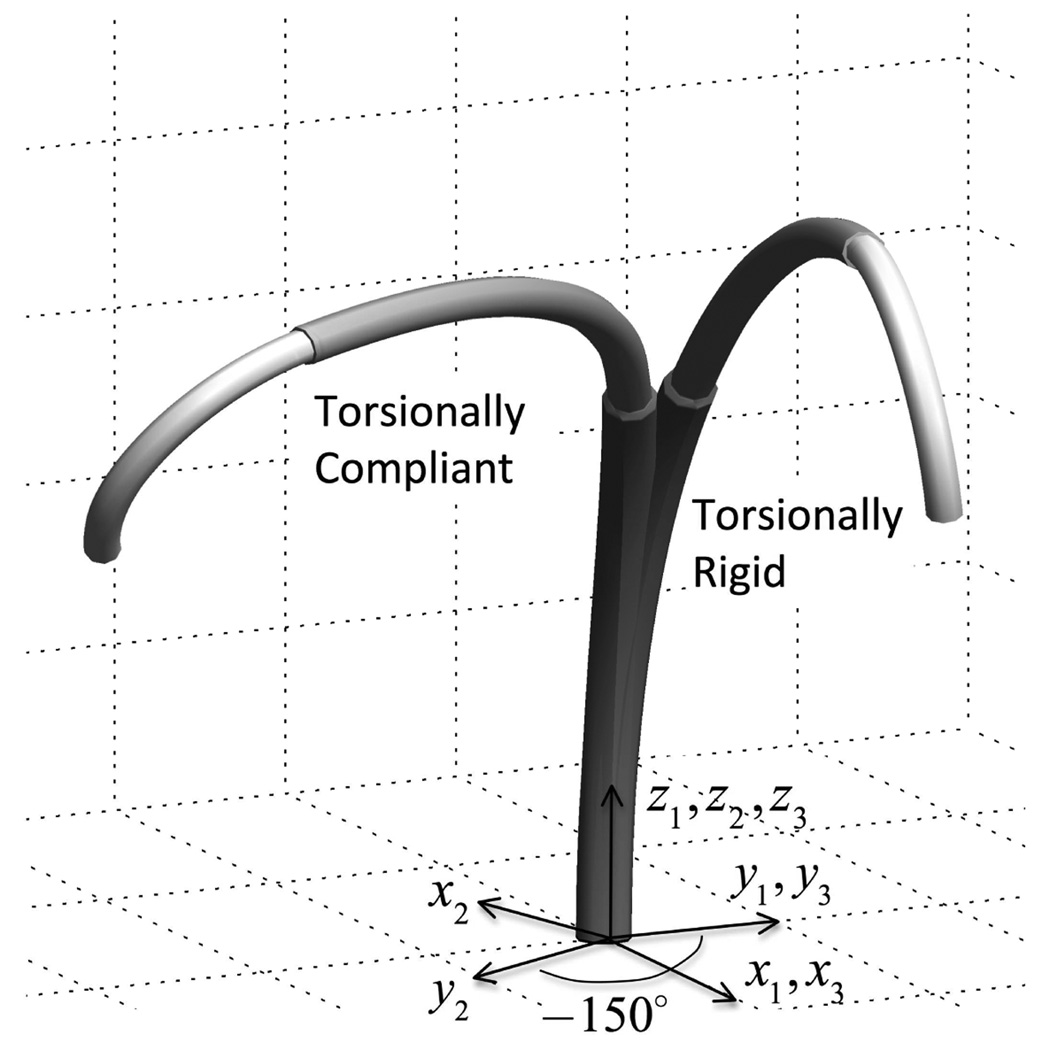
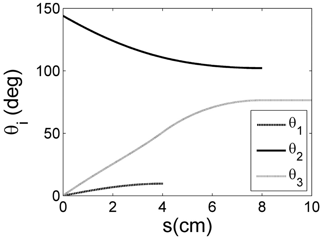
To compare the predicted shapes of the torsionally compliant model with that of the torsionally rigid model, the results of a three-tube simulation are shown in Fig. 3 and Fig. 4. Equation (7) was used to compute the curvature the torsionally rigid model which was then analytically integrated as described in [6] to solve for the location of the robot in space. For the torsionally compliant model, an iterative method was used with (52) to determine the tip rotation angles θ_i(L_i) that produced the desired base rotation angles θ_i(0). The resulting curvatures were then integrated numerically from the base to the tip to compute the shape of the robot.

Fig. 3.

Three-tube robot comparing torsionally rigid and compliant models.

Fig. 4.

Tube twist angle versus arc length.

The parameters for the simulation are given in Table 1. The bending stiffnesses were selected since they are representative of values that could arise in robot design. The lengths of the tubes were selected such that more flexible tubes extend telescopically from stiffer tubes. The tubes’ curvatures are constant over the entire lengths and the coordinate frames are defined such that when the initial curvatures of the tubes are aligned, the rotation angles at the base are all zero, θ₁ = θ₂ = θ₃ = 0. The configuration noted in the table and depicted in Fig. 3 and Fig. 4 corresponds to rotating tube 2 at the base by −150 degrees. As shown in the figures, this configuration demonstrates substantial variation in twist angle for all overlapping portions of the tubes.

TABLE 1.

TUBE PARAMETERS FOR SIMULATION.

Tube	1 (outer)	2	3 (inner)
Relative Stiffness	5	3	1
Initial Curvature (cm)	5	9	1
Length (cm)	4	8	10
Base Rotation, θi (degrees)	0	−150	0

IV. ANALYTICAL SOLUTION FOR TWO TUBES OF PIECEWISE CONSTANT CURVATURE

The differential equation governing the twist of two constant curvature tubes, repeated here,

$$\ddot{\alpha }(s)=(1+\nu )\Vert {\widehat{u}}_1\Vert \Vert {\widehat{u}}_2\Vert \text{sin}\alpha (s)=c\text{sin}\alpha (s)$$ (56)

has two trivial equilibrium solutions

$$\alpha (s)=\{0,\pi \},s\in [0,L]$$ (57)

These correspond to the situations in which the cross sectional curvature vectors of the tubes have the same and opposite direction, respectively. In neither case is an external torque needed to maintain the configuration. One can guess, however, that the solution α(s) = π is not a minimum energy solution for the kinematic input value α(0) = π and thus it is likely that additional solutions to (56) share the initial condition α(0) = π.

To study solution multiplicity, we seek an analytic solution to (56). To integrate by separation of variables, we use $\ddot{\alpha }=\dot{\alpha }\frac{d\dot{\alpha }}{d\alpha }$ and write

$${\displaystyle \underset{\dot{\alpha }(0)}{\overset{\dot{\alpha }(s)}{\int }}\dot{\alpha }d\dot{\alpha }=c}{\displaystyle \underset{\alpha (0)}{\overset{\alpha (s)}{\int }}\text{sin}\alpha d\alpha }$$ (58)

This results in the following expression for α̇(s)

$${\dot{\alpha }}^2(s)={\dot{\alpha }}^2(0)+2c(\text{cos}(\alpha (0))-\text{cos}(\alpha (s)))$$ (59)

Evaluating this equation using the boundary condition α̇(L) = 0 and substituting the result in (59) yields

$${\dot{\alpha }}^2(s)=2c(\text{cos}(\alpha (L))-\text{cos}(\alpha (s)))$$ (60)

Separation of variables can be used again to obtain

$$s=\frac{\pm 1}{\sqrt{2c}}{\displaystyle \underset{\alpha (0)}{\overset{\alpha (s)}{\int }}\frac{d\alpha }{\sqrt{\text{cos}(\alpha (L))-\text{cos}(\alpha )}}}$$ (61)

In (61), the sign is selected to match the sign of the integration interval, sgn(α(s) − α(0)). Recognizing (61) as an elliptic integral of the first kind, we desire an expression for the upper limit of integration, α(s). This can be obtained in terms of Jacobi elliptic functions by a variety of methods including converting the integral of (61) to standard form or by assuming a solution and showing that it satisfies (60). This results in

$$\text{sin}(\alpha (s)/2)=\text{sin}(\alpha (L)/2)/\text{dn}\left((L-s)\sqrt{c}|{\text{cos}}^2(\alpha (L)/2)\right)$$ (62)

in which dn(u | m) is a Jacobi elliptic function [1]. Equation (62) expresses relative twist angle in terms of the twist angle at the distal end and is well posed since dn (u | m) > 0. We are specifically interested in the value at the proximal end since it is the kinematic input, α(0) = θ₂(0) − θ₁(0).

$$\text{sin}(\alpha (0)/2)=\text{sin}(\alpha (L)/2)/\text{dn}\left(L\sqrt{c}|{\text{cos}}^2(\alpha (L)/2)\right)$$ (63)

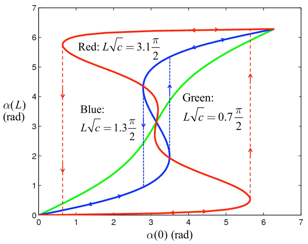
his expression involves a single dimensionless parameter $L\sqrt{c}$ . Fig. 5 plots (63) for several values of this parameter. It can be seen that at least one value of α(L) exists for each value of α(0) ∈ [0,2π], but it is also apparent that there can be multiple solutions. Solution multiplicity produces sudden changes in tube twist in response to incremental changes in the kinematic input, α(0). These “snap through” instabilities are indicated as dashed lines in the figure and correspond to the tubes traversing between minimum energy branches of the curve.

Fig. 5.

Tip versus base twist angle.

To determine the dependence of “snap through” on the parameter Lc^1/2, we count the solutions for α(L) given α(0) = π. Equation (63) reduces to

$$\text{sin}\left(\alpha (L)/2\right)=\text{dn}\left(L\sqrt{c}|{\text{cos}}^2(\alpha (L)/2)\right)$$ (64)

Since dn(u | 0) = 1, (64) always has at least one solution {α(0), α(L)} = {π, π} corresponding to no torsional twist along the tubes’ length. To determine when additional solutions exist, we use the identity [1]

$$\begin{array}{c}\text{dn}(K(m)|m)=\sqrt{m_1}\hfill \\ m+m_1=1,0\le m\le 1\hfill \end{array}$$ (65)

and note that dn is periodic in its first argument with period 2K(m). Here, K(m) is the complete elliptic integral of the first kind which is a monotonically increasing function of m with K(0) = π / 2 and K(1) = +∞. Combining (64) and (65) results in

$$L\sqrt{c}=\mathit{\text{nK}}(m),n=1,3,5,\dots$$ (66)

This equation has no solutions for $L\sqrt{c}<\pi /2$ and for $L\sqrt{c}=\pi /2$ the n = 1 solution is identical to the original solution {α(0), α(L)} = {π, π}. For $\pi /2<L\sqrt{c}\le 3\pi /2$ , one new solution to (66) exists. Since m = sin² (α(L) / 2), this yields two new solutions, $\text{sin}\left(\alpha (L)/2\right)=\pm \sqrt{m}$ . As seen in Fig. 5, these solutions are symmetric about α(L) = π. Similarly, $3\pi /2<L\sqrt{c}\le 5\pi /2$ yields four solutions to (66).

The dimensionless parameter $L\sqrt{c}=\pi /2$ is very important from a design perspective. The model predicts that tubes for which $L\sqrt{c}<\pi /2$ will not exhibit “snap through.” As this parameter increases, additional solutions exist which lie on unstable branches of the relation. The critical values of α(0) for “snap through” correspond to the extrema of α(0) adjacent to the n = 1 solutions of (66).

V. EXPERIMENT

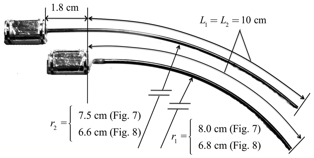
To validate the behavior predicted in Fig. 5, tests were performed on two tube pairs shown in Fig. 6. Each tube is glued into a collar as shown and mounted in the motor drive system described in [9]. Motor positioning accuracy is better than 0.1 degrees. Equation (63) must be adjusted to relate α(0) measured at the proximal end of the curved portion of the tubes to the relative angle measured by the motor encoders at the tube collars, α_m. This is given by

$${\alpha }_m=\alpha (0)-\dot{\alpha }(0)(18\text{mm})k_{2z}/(k_{1z}+k_{2z})$$ (67)

Unlike (63), this computation requires the stiffness ratio of the tubes. The outer diameters of the tubes were measured with a micrometer to be 1.455 and 1.257 mm. The inner diameters of 1.346 and 1.067 mm were estimated by inserting drill bits of the largest available diameter inside the tubes and using a micrometer to measure the diameter of the bits. Thus, the ID measurement is less precise and suggested a stiffness ratio between 0.8:1 and 1.2:1. Computation shows that this variation produces a difference in α_m of at most one degree.

Fig. 6.

Dimensions of two tube pairs.

To measure the twist at the distal end of the tubes, α(L), a circular graduated disk was attached over the last 2 mm of the outer tube. A pointer attached to a tapered dowel was inserted into the end of the inner tube and zeroed for the configuration in which the curvature of the tubes is aligned. The error in measuring tip angle was estimated to be ±2 degrees.

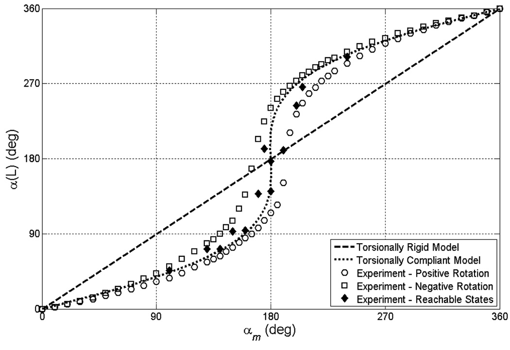
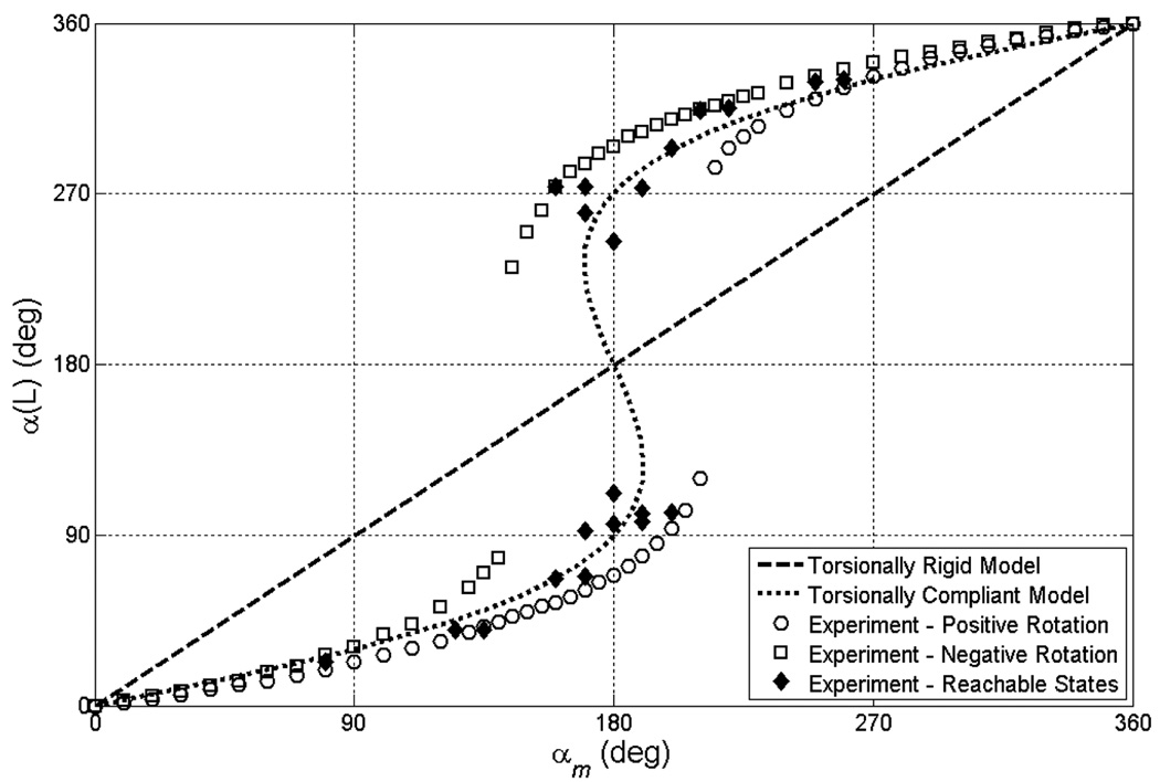
Fig. 7 and Fig. 8 compare the torsionally rigid and compliant models with experiment for stable and unstable pairs of tubes, respectively. The torsionally rigid model is a line of unit slope while the torsionally compliant model obtained from (63) and (67) predicts s-shaped curves. Experimental data was collected by rotating the tube pairs quasistatically through a complete revolution in the positive and negative directions. This data produced an envelope of the possible reachable values of (α_m, α(L)). The envelope is due to unmodeled hysteretic phenomena. Also shown are additional data points collected through sequences of motions within the envelope. These points demonstrate that the entire interior of the envelope in Fig. 7, including the point (α_m, α(L)) = (π, π), is reachable and stable. In contrast, there are stable and unstable portions of the envelope in Fig. 8.

Fig. 7.

Tip versus motor twist angle for a stable tube pair.

Fig. 8.

Tip versus motor twist angle for an unstable tube pair.

VI. CONCLUSION

The torsional kinematic model presented here provides substantial improvement in predictive power in comparison to the torsionally rigid model. It also enables analytic prediction, through the dimensionless parameter $L\sqrt{c}$ , of the existence of instability as well as the stable range of kinematic input parameters. While the model requires the integration of a two-point boundary value problem, it is likely that efficient techniques can be developed to enable its application to both robot design and real-time control.

REFERENCES

- 1.Abramowitz M, Stegun IA. Handbook of mathematical functions. New York: Dover Publications, 9th printing; [Google Scholar]
- 2.Antman SS. Nonlinear problems of elasticity. New York: Springer Verlag; 1995. [Google Scholar]
- 3.Ebrahimi R, Okzawa S, Rohling R, Salcudean SE. Handheld Steerable Needle Device. Medical Image Computing and Computer Assisted Intervention. 2003:223–230. [Google Scholar]
- 4.Loser M, Navab N. A New Robotic System for Visually Controlled Percutaneous Interventions under CT Fluoroscopy. Medical Image Computing and Computer-Assisted Intervention. 2000 [Google Scholar]
- 5.Loser M. Dr. Ing. Dissertation, Microsystems Technology. Germany: U. Freiburg; 2005. A New Robotic System for Visually Controlled Percutaneous Interventions under X-ray Fluoroscopy or CT-imaging. [Google Scholar]
- 6.Sears P, Dupont P. A Steerable Needle Technology Using Curved Concentric Tubes. IEEE/RSJ Int. Conference on Intelligent Robots and Systems; Beijing. 2006. pp. 2850–2856. [Google Scholar]
- 7.Webster RJ, Okamura AM, Cowan NJ. Toward Active Cannulas: Miniature Snake-Like Surgical Robots. IEEE/RSJ Int. Conf. Intelligent Robots and Systems; Beijing. 2006. pp. 2857–2863. [Google Scholar]
- 8.Sears P, Dupont P. Inverse Kinematics of Concentric Tube Steerable Needles. IEEE 2007 International Conference on Robotics and Automation; Roma, Italy. 2007. pp. 1887–1892. [DOI] [PMC free article] [PubMed] [Google Scholar]
- 9.Itkowitz B. MS Thesis. Boston, MA: Electrical & Computer Eng, Boston Univ.; 2007. Teleoperation of Concentric Tube Manipulators. [Google Scholar]
- 10.Mahvash M, Dupont P. Bilateral Teleoperation of Flexible Surgical Robots. Workshop Proc, New Vistas and Challenges in Telerobotics; IEEE 2008 International Conference on Robotics & Automation; 2008. pp. 58–64. [Google Scholar]
- 11.Webster RJ, III, Romano JM, Cowan NJ. Kinematics and Calibration of Active Cannulas. IEEE International Conference on Robotics and Automation; 2008. pp. 3888–3895. [Google Scholar]
- 12.Webster RJ, III, Swensen JP, Romano JM, Cowan NJ. Closed-Form Differential Kinematics for Concentric-Tube Continuum Robots with Application to Visual Servoing. 11th Int. Symposium on Experimental Robotics; Athens, Greece. 2008. [Google Scholar]