

Abstract
A variant of the popular nonparametric nonuniform intensity normalization (N3) algorithm is proposed for bias field correction. Given the superb performance of N3 and its public availability, it has been the subject of several evaluation studies. These studies have demonstrated the importance of certain parameters associated with the B-spline least-squares fitting. We propose the substitution of a recently developed fast and robust B-spline approximation routine and a modified hierarchical optimization scheme for improved bias field correction over the original N3 algorithm. Similar to the N3 algorithm, we also make the source code, testing, and technical documentation of our contribution, which we denote as “N4ITK,” available to the public through the Insight Toolkit of the National Institutes of Health. Performance assessment is demonstrated using simulated data from the publicly available Brainweb database, hyperpolarized 3 He lung image data, and 9.4T postmortem hippocampus data.
Index Terms: B-spline approximation, bias field, inhomogeneity, N3
I. Introduction
A potential confounder in various image analysis tasks is the presence of a low frequency intensity nonuniformity present in the image data also known as bias, inhomogeneity, illumination nonuniformity, or gain field (Fig. 1). For a review of intensity inhomogeneity artifacts and a relatively recent discussion of existing correction methods, see [1]–[3] and the references contained therein.
Fig. 1.

(a) T1-weighted MR image exhibiting bias. (b) Several algorithms have been proposed to estimate the bias field which can then be used to “correct” the image. (c). Viewed as a surface, the low frequency modulation of the bias field is readily apparent.
Amongst the various bias correction algorithms that have been proposed in the research literature, the nonparametric nonuniform normalization (N3) approach formulated in [4] has established itself as a de facto standard in the field. Comparative evaluation studies involving N3 have consistently demonstrated its relatively superb performance for a variety of imaging acquisition strategies applied to a spectrum of imaging subjects (e.g., [5]–[7]). The wide popularity of N3 is due not only to its performance but also its ease of use and its availability as open source supported by the McConnell Brain Imaging Centre of the Montreal Neurological Institute which has an established track record of availing image analysis and visualization software tools to the research community.1
Evaluation studies have investigated different aspects of the algorithm. Specifically, in [5], the investigators evaluated six bias correction algorithms (including N3) for phantom data and subject brains imaged using both 1.5T and 3.0T magnetic resonance imaging (MRI) scanners at two different sites. N3 performed consistently well for all experimental scenarios using the default parameters originally proposed in [4]. In [6] the performance of N3 for 3.0T brain MRI data with variation in the selected mask and the spline distance, i.e., the distance between the knots defining the B-spline mesh. As noted by the authors, greater field strength results in a higher frequency modulation of the corrupting bias field. Thus, it was found that decreasing the spline distance from 200 mm to the range 50–100 mm [see Fig. 2(b) and (c)] led to statistically significant improved results. It was also found that segmentation strategies isolating distinct tissue classes within the image and using those single-tissue regions as masks for the N3 algorithm improved the bias correction results. Dovetailing this study was the exploration in [7] which found improved 3.0T MRI brain segmentation results derived from the Freesurfer2 segmentation pipeline using N3 distances in the range 30–50 mm [see Fig. 2(c) and (d)] with much smaller distances causing N3 to fail.
Fig. 2.

Illustration of the spline distance parameter of N3 relative to typical brain anatomy. For uniform B-splines (which are employed by N3), spline distance, i.e., control point spacing, is identical with the mesh element size. Several commonly used N3 spline distances are overlaid on an axial brain slice: (a) 150 mm, (b) 100 mm, (c) 50 mm, and (d) 30 mm. Not shown is the default N3 control point spacing of 200 mm.
The authors of a recent review of bias correction methods write of N3 [3]:
A well-known intensity inhomogeneity correction method, known as the N3 (nonparametric nonuniformity normalization), was proposed in [15]. The method is iterative and seeks the smooth multiplicative field that maximizes the high frequency content of the distribution of tissue intensity. The method is fully automatic, requires no a priori knowledge and can be applied to almost any MR image. Interestingly, no improvements have been suggested for this highly popular and successful method.
In this contribution, we attempt to improve the original N3 algorithm by replacing the B-spline smoothing strategy used in the original N3 framework with an advantageous alternative [8]–[10] which addresses major issues explored by previous N3 evaluation studies. In addition, we modify the iterative optimization scheme which, among other things, improves convergence performance. Of most practical significance is that, similar to the original N3 offering (which we denote throughout the remainder of this work as “N3MNI” for clarification purposes), we developed our N3 algorithm within the open source Insight Toolkit of the National Institutes of Health for public dissemination, vetting, and improvement [11]. As such, we denote our N3 variant as “N4ITK” [12].
II. Overview of Contribution
The image formation model assumed by N3, which is also common to other bias correction algorithms [3], is
| (1) |
where v is the given image, u is the uncorrupted image, f is the bias field, and n is the noise (assumed to be independent and Gaussian). Using the notation û = log u and assuming a noise free scenario, the image model becomes
| (2) |
From this model, the following iterative solution is derived in [4] for obtaining the corrected image at the nth iteration
| (3) |
where û0 = v̂, (the initial bias field estimate) is typically set to 0, and the smoothing operator, S{·}, is a B-spline approximator. The derivation of the expected value of the true image given the current estimate of the corrected image, E[û|ûn−1], is also given in [4].
The two principal contributions that we make are readily seen by comparing the iterative scheme of N3MNI given by (3) with the scheme we propose for N4ITK, i.e.,
| (4) |
where S*{·} is a different B-spline approximator (which we have also made publicly available) and is the estimated residual bias field at the nth iteration (in contrast, N3MNI re-estimates the total bias field, , at the nth iteration).
Replacing S{·} with S*{·} allows for smaller control point spacing to accommodate greater field strengths without the possibility of algorithmic failure, obviates the need for an artificial regularization parameter, and permits the specification of a weighted regional mask for possible use within an iterative segmentation framework. Additional advantages include faster execution times due to parallelization of our B-spline approximation algorithm and a multiresolution approximation strategy for hierarchical fitting of successively higher levels of frequency modulation of the bias field.
The latter advantage is related to our second contribution which is a modified optimization scheme to accommodate an iterative incremental update of the bias field. we have found that this improves convergence behavior over the N3MNI algorithm.
We provide further details of both contributions in subsequent sections. Specifically, the differences in B-spline approximation approaches are elucidated in Section III and the iterative schema for both algorithms are compared in Section IV.
III. B-Spline Approximation
Given a set of uniformly or nonuniformly distributed data samples, the process of reconstructing a function from those samples finds diverse application in generic quantitative data analysis. Due to many of their salient properties, parameterized reconstruction techniques employing B-splines have continued to find application since Riesenfeld first introduced B-splines to approximation problems in computer-aided design [13].
B-spline objects are defined by a set of B-splines and a grid of control points. B-splines can be derived recursively by a stable algorithm known as the Cox-de Boor recurrence relation [14], [15]. After specifying the order of spline (which we denote by d) and a knot vector U = {U1, …, Um} the B-splines are given by
| (5) |
where
| (6) |
Uniform B-splines are characterized by knot elements being equally spaced, i.e., Ui+1−Ui = c ∀ i ∈ {1, m − 1} for some constant c. This constraint simplifies the B-spline calculation. Since uniform B-splines are used in both N3MNI and N4ITK, we restrict our discussion accordingly.
In reconstructing the parameterized object, the B-splines serve as weighted smoothing functions for the set of control points. As an example, a B-spline surface is a bivariate function given by
| (7) |
The generalized formulation of a B-spline object of n-dimensions is
| (8) |
where the set P and the distinct B parametric functions respectively denote the controls points and B-splines. Given the advantageous properties of B-splines, various approximation and interpolation algorithms have been developed to fit B-spline objects to scattered data.
A. Least Squares B-Spline Data Approximation
An early technique for approximation of scattered data using B-splines is based on the minimization of the sum of the squared residuals between the individual data points and the corresponding function values defined by the B-spline object (commonly referred to as least squares fitting). Such techniques involve the construction of a linear system of equations from a set of data points. Standard matrix transformations are then used to solve for the values of the governing control points. Specifically, given a set of N data points specified by S = {s1, …, sN} and the corresponding parametric values U = {u1, …, un}, the values of the control points can be found by minimizing
| (9) |
Evaluating the gradient of E(P) and setting the result to 0 yields the following linear system
| (10) |
where B is the observation matrix comprised of the products of B-spline values at the parametric values, U. The pseudoinverse solution of this system is given by
| (11) |
A drawback to this strategy is that locally insufficient data point placement can lead to ill-conditioned matrices producing undesirable results.3 Formally, this is described by the Schoenberg-Whitney conditions. These conditions concern the placement of the data within the parametric domain, violation of which causes an underdetermined linear system leading to solution instability. A practical discussion of the Schoenberg-Whitney conditions is given in [16].
To avoid such instability problems various explicit regularization strategies have been adopted. For example, in N3MNI, a weighted regularization term, ωR(P), is added such that the minimization problem becomes
| (12) |
where R is the thin plate energy of the B-spline object. However, such parameters introduce an artificial stiffness to the fitting solution. This added stiffness, although necessary in areas of insufficient data, negatively affects the fidelity of the B-spline object to the scattered data and are difficult to tune [17].
B. Fast and Robust Generalized n-D Ck B-Spline Data Approximation
Lee et al. proposed a uniform B-spline approximation algorithm in [8] which circumvents the problematic issues associated with conventional least squares fitting for 2-D cubic B-spline scalar objects. The authors also introduce this algorithm within the context of a multilevel framework for hierarchical surface fitting. While they discuss the possibility of extending their algorithm to multiple parametric and data dimensions, both the details of the implementation of their algorithm as well as the applications are restricted to cubic B-spline scalar fields (bivariate functions).
Our contribution, initially discussed in [10] and given to the research community in [9], comprises a parallelized generalization of Lee’s original algorithm. In Section III-BI, we review the basics of the algorithm discussed in [8] while noting the generalizations made in our contribution.
1) Extension to Multivariate B-Spline Objects With Confidence Values
For a single isolated data point in n dimensions to be approximated by a B-spline object, one can solve for the values of the surrounding subset of control points. Due to the underdeterminedness of the corresponding linear system, an infinite number of solutions is possible. However, the solution determined by the pseudoinverse results in a solution which is optimal in a least-squares sense (i.e., the magnitude of the solution vector is minimized). Based on (8), we can write the single data point situation as follows:
| (13) |
where Sc is the single data point under consideration and is located in the parametric domain at ( ). Note that the summation indices are only over a subset of the m-D grid of control points determined by the order of spline used in each parametric dimension. More specifically, in dimension j, dj + 1 indices will be considered. Also, note that discussion of dimensionality concerns both the spatial and parametric domains denoted by n and m, respectively. For example, a B-spline curve is specified by a function of a single parameter (m = 1) while residing in 3-D space (n = 3).
Rewriting (13) in matrix notation yields
| (14) |
where S is the single data point vector of size 1 × n, B is the B-spline row matrix of size , and P denotes the control point values of size . Similar to the multiple data points scenario in the previous section, the pseudoinverse solution for a single data point is given by
| (15) |
or by the equivalent summation notational form
| (16) |
However, the facility of solving the single data point problem does not generalize to irregularly placed data where, generally speaking, multiple data points will correspond to overlapping control points. In contrast to isolated data points, such a scenario requires finding a solution which provides an approximation to this subset of data points. The control point value is that which minimizes the sum of the squared difference for each of the proximal C data points between the isolated function value, i.e., the function value calculated from (13) assuming the control point is isolated, and the function value calculated from the minimizing control point value. We also add a confidence term, δ, for each of the data points which produces the minimization criterion
| (17) |
Minimization leads to the solution for Pi1, …,im
| (18) |
2) Extension to Arbitrary Order
The original formulation in [8] restricted discussion to cubic B-splines. Such a restriction is a natural choice since it can be shown that a cubic curve which interpolates a set of data points also minimizes its curvature [18]. Although the default spline order is cubic in both N3MNI and N4ITK, we recognize that exploration of noncubic B-splines might prove useful for a particular application (e.g., [19]). Therefore, we extended the original cubic implementation to arbitrary order.
3) Multiresolution Approximation
The original multilevel approach is extended to arbitrary dimension and arbitrary spline order where each successive level is characterized as having twice the mesh resolution of the previous level. In ascending to the next higher level of higher resolution, the initial step requires calculating the new control point values which produce the same B-spline object with a higher control point resolution. The description in [8] only provides the coefficients for calculating the higher resolution cubic B-spline surface from the lower resolution surface. Discussion in [20] describes the derivation of the coefficients for both the univariate and bivariate cubic B-spline case. We present a brief discussion of doubling the resolution for multivariate B-spline objects of arbitrary order.
At a given resolution level, the B-splines are simply scaled versions of the B-splines at the previous value such that where B′ is the B-spline at the higher level. Thus, for each polynomial span in 1-D, finding the nodal values entails first formulating the following equality:
| (19) |
Grouping the monomials of the separate B-splines on both sides of the equality and setting like groups of terms equal to each other, we obtain the following linear system:
| (20) |
where it is assumed that the B-splines are expressed in polynomial form, i.e., Bi,d(u) = bd+1,iud + bd,iud−1 + … + b1,i.This relatively small system is easily solved using standard matrix routines. Since each uniform B-spline is simply a parametric translation of a single representative B-spline function and since each B-spline is symmetric with respect to its maximum value, the matrix obtained from multiplying the inverse of the B-spline coefficient matrix on the left side of (20) with the B-spline coefficient matrix on the right side contains consists of “translated” row pairs. Therefore, one can simply use the top two rows of coefficients of the resulting matrix product to calculate the control point values at the given level from the control point values at the previous level. Extending this formulation to the multivariate case is fairly straightforward. One simply calculates the tensor product of the relevant row of coefficients for each dimension. The coefficients for the multivariate (n-D) case are given by the elements of the n-tensor
| (21) |
where Ci is one of the two rows of coefficients for the ith dimension and ⊗ denotes the outer or tensor product between two vectors. Note that different dimensions might employ different orders of B-splines. Similarly, transcending one level might require refinement in one parametric dimension but not in the other. These two cases are also handled by our algorithm.
C. Comparison of the Two B-Spline Approximation Algorithms With Relevance to N3 Bias Correction
Our proposed B-spline approximation algorithm substitution in N4ITK provides several advantages over the approximation strategy used in N3MNI. Due to potential violation of the Schoenberg-Whitney conditions, the N3MNI approximation scheme requires the use of an artificial smoothing contribution based on penalizing the thin-plate energy of the B-spline object. Although this explicit regularization mitigates ill-conditioning of the resulting linear system, it negatively affects the fidelity of the solution fit to the underlying scattered data and does not guarantee a stable solution. Relevant is the difficulty of tuning the regularization weighting parameter, ω, simultaneously with the spline distance. Our substitution eliminates this parameter.
Another difference between the two B-spline approximation algorithms is the well-known susceptibility to outliers of the total least-squares approach. Such susceptibility negatively affects the solution particularly for noisy images. In contrast, the approximation algorithm used by N4ITK is more robust to noise since approximation is performed initially at the local level followed by merging of the local solutions [8] as opposed to an initial global fit as with total least-squares. This advantage is demonstrated in the results of the experimental section comparing the two algorithms.
Of related additional interest is the ability to associate data points with confidence values. Instead of simply specifying a binary mask designating the bias field estimation region, with N4ITK one can specify a confidence mask. This could be potentially useful in an iterative soft segmentation framework where, at each iteration, a membership value for a single tissue class is assigned to each voxel. One could then perform N3 bias correction at each iteration using the membership values for a single tissue class. We leave this exploration for future work.
IV. Multiresolution Optimization With Incremental Update of the Bias Field Estimate
The iterative solution employed by N3MNI is given by (3). Thus, the first iteration yields
| (22) |
For the second iteration, N3MNI utilizes the corrected log image, û1, to re-estimate the expected value of the true field, E[û|û], from which one would then re-estimate the total bias field, . This process continues where the total bias field is re-estimated at each iteration, i.e.,
| (23) |
We found that improved results can be achieved with N3MNI if the algorithm is run more than once where the input image of the second run is the corrected image of the first run and so on. We realized that this heuristic could lead to a second iterative option which we adopt in N4ITK. Subsequent to the identical first iteration (with S{·} replaced by S*{·}), we perform a bias correction step on the corrected image from the previous iteration to estimate the residual bias field, f̂r, at the current iteration such the iterative scheme of N4ITK becomes
| (24) |
Instead of convergence to the total bias held, our iterative scheme is designed to converge such that where calculation of the total bias field estimate is seen by inspecting the nested nature of (24), i.e.,
| (25) |
Thus, the total bias held estimate at the nth iteration is the sum of the first n residual bias fields, i.e.,
| (26) |
Due to the additive equivalence between the B-spline objects and their control point values, we simply maintain a running summation of the control point lattice values during the optimization.
We have noticed improved convergence with this approach. In detailing the theoretical components of the algorithm [4], convergence is determined by the coefficient of variation in the ratio between subsequent bias field estimate voxel values. However, in actual implementation, convergence in N3MNI is determined from the standard deviation alone due to the erratic behavior of the coefficient of variation during the course of optimization. In contrast, our implementation actually uses the theoretical convergence criterion.
A related feature which takes advantage of our proposed approximation algorithm and the new iterative scheme is the multiresolution fitting component which is similar to other approaches [21], [22]. As noted in previous studies, greater field strengths result in higher frequency modulation necessitating smaller spline distances (i.e., higher B-spline mesh resolutions) to model such modulation. However, direct fitting using a higher mesh resolution might miss the lower frequency components of the underlying field. This is demonstrated in Fig. 3 where solution values default to 0 in areas of no data. Given the scattered data points in Fig. 3(a) and a relatively high resolution B-spline mesh of 32 × 32 elements, an accurate, but highly localized, fit to the data can be achieved in Fig. 3(b). However, a different solution is obtained with the same B-spline mesh of 32 × 32 elements using hierarchical fitting. This approach captures a range of approximation to the data from global to localized by initially fitting a low-resolution B-spline object to the data followed by approximation with increasing mesh resolutions. In this sense, N4ITK can use a range of spline distances to achieve the “best” fit as opposed to a single spline distance. Such a fit is seen in Fig. 3(c) where we started with a low resolution B-spline mesh (lxl element) and continued the fitting for five additional levels for a final mesh resolution of 32 × 32 elements.
Fig. 3.
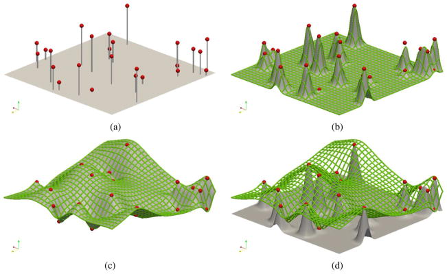
Comparison of fitting strategies for a simple 2-D scattered point set example. (a) Set of 25 scattered data points. (b) Highly localized approximation using a single level 32 × 32 element B-spline mesh. (c) Approximation by a hierarchy of B-spline mesh resolutions starting from a single B-spline mesh element and ending with a 32×32 element B-spline mesh. (d) Superposition of the fitted B-spline mesh from (c) and the fitted surface from (b) to illustrate the discrepancy in solutions.
Putting both components together, the multiresolution iterative optimization framework is given as pseudocode in Algorithm 1. The control point lattice representing the total bias field estimate is denoted by f̂e(p) whereas the control point lattice representing the residual bias field estimate is denoted by f̂r(p).
Algorithm 1.
N4ITK Multiresolution Optimization
| 1: f̂e(p) ← 0 {initialize control point lattice} |
| 2: n ← 1 |
| 3: for each resolution level do |
| 4: for each iteration at current resolution level do |
| 5: |
| 6: |
| 7: |
| 8: n ← n + 1 |
| 9: end for |
| 10: f̂e(p) ← f̂e(p)′ {refine control point lattice} |
| 11: end for |
V. Experimental Comparison
Our first set of experiments utilizes the BrainWeb simulated phantom data. Given the public availability of these data and their use in previous N3 evaluations, this set of experiments is used for establishing a benchmark comparison between N3MNI and N4ITK. Experimentation using real data includes hyperpolarized 3He MRI of the lung and labeled hippocampus data acquired at 9.4T [23]. The high field strength characterizing the acquisition of the latter data causes exceptionally strong bias and provides a unique set of test data to compare N3MNI and N4ITK.
For all comparative experiments, we used N3MNI downloaded from the MNI website (version 1.11.0, uploaded 29 July, 2009). N4ITK is available through the online Insight Journal (http://hdl.handle.net/10380/3053). In addition to the spline distance and regularization parameters previously discussed, the remaining defining parameters of N3MNI include the following:
image mask;
shrink factor—integer quantity defining the subsampling of the original image used to decrease computational time;
full width at half maximum—quantity characterizing the deconvolution kernel;
convergence threshold—quantity determined by the coefficient of variation of the ratio of the intensity values between subsequent field estimates;
maximum number of iterations.
Each of these parameters is also used in N4ITK. Further information regarding the parameters can be found in [12] and [4].
A. Brain Web Phantom and Simulated Bias Field Data
A component of the evaluation in [5] involved comparing known bias fields with the extracted bias fields produced by the six bias correction algorithms being studied using the Brainweb database [24]–[26].4 Similar to that study, our first experimental comparison used the 20 recently developed Brainweb normal subjects (1 mm isotropic spacing, no added noise, discrete anatomical labeling) in conjunction with the three simulated bias fields, also available from the Brainweb database, labeled “A,” “B,” “C,” [25], [26].
From these images, a set of experiments were performed to compare the performance of N3MNI and N4ITK for a set of commonly used spline distances (50, 100, and 200 mm—see Fig. 2) in the presence of additive Gaussian noise as assumed by the image formation model [see (1)]. To create the experimental data, each of the 20 images was resampled to the size of the given bias fields. Each resampled image was then rescaled to the range [0,100] with white matter having the largest intensity value and subsequently multiplied by one of the three bias fields which had been linearly rescaled to the range [0.9,1.1] for a 20% bias field or [0.8,1.2] for a 40% bias field. Each biased image was then corrupted using Gaussian noise characterized by one of three noise levels:  (0,5),
  (0,10), and
  (0,20).
Bias correction was performed for all created image data using both algorithms (20 subjects x 3 noise levels x 3 bias fields x 2 bias field strengths x 3 spline distances x 2 algorithms = 2160 total bias correction). Both N3MNI and N4ITK were employed with the default parameters for both algorithms (except those parameters specific to the respective B-spline approximation algorithms): full width at half maximum = 0.15, convergence threshold = 0.001, maximum number of iterations = 50, and shrink factor = 4. The region mask used by both algorithms was defined for each run by the nonzero pixels of the specific subject. The spline distances of 50, 100, and 200 mm were achieved with N4ITK by starting with a single B-spline mesh element of 200 mm x 200 mm and performing 1, 2, and 3 multiresolution levels, respectively, where the 200 iterations were divided equally among the different resolution levels.
All bias corrections (including those discussed in later sections) were performed on a computational cluster housed at Penn Image Computing and Science Laboratory (PICSL) which consists of 32 nodes, each node consisting of two quad-core 2.8-GHz Intel processors and 16 GB of memory. Because of this computational setup, threading capabilities are removed limiting the speed-up of N4ITK due to our multithreaded B-spline approximation algorithm. However, despite this constraint, the average time (± standard deviation) for all experiments performed on the BrainWeb data using N4ITK was 23 (±8.8) seconds per bias correction. In contrast, the time statistics for N3MNI were 46 (±27) seconds per bias correction.
Agreement of the recovered bias fields with the ground truth bias fields was assessed by calculating the correlation coefficient between the two fields over the masked region. These results are given in the box plots of Fig. 4 (20% bias) and Fig. 5 (40% bias) with the algorithmic results paired according to simulated bias field. The top and bottom box limits are calculated from the 25th and 75th percentiles of the data (q25% and q75%) respectively) and the median value is denoted by the horizontal dashed line. The extent of the box plot whiskers is given by the range [q25%−1.5 · (q75%−q25%), q75%+1.5 · (q75%−q25%)]. Any datum outside that range is typically considered an outlier and is denoted by the “+” symbol. Although N3MNI achieves better correlation values for the 5% noise level and spline distance of 200 mm, the trend appears to be that increasing the noise (which includes the absolute noise level as well as the noise relative to the bias field strength) and decreasing the spline distance N4ITK consistently outperforms N3MNI.
Fig. 4.

20% bias field results: Correlation coefficient analysis for the BrainWeb data with varying levels of additive Gaussian noise and spline distances where the simulated bias fields were linearly rescaled to [0.9,1.1]. Results are paired by bias field with the results of N4ITK given in blue and the corresponding N3MNI results given in green. Although N3MNI performs comparatively well for the 5% noise level and spline distance = 200 mm, with increasing noise and increasing mesh resolution (i.e., decreased spline distance), N4ITK consistently achieves improved results.
Fig. 5.

40% bias field results: Correlation coefficient analysis for the BrainWeb data with varying levels of additive Gaussian noise and spline distances where the simulated bias fields were linearly rescaled to [0.8,1.2]. Results are paired by bias field with the results of N4ITK given in blue and the corresponding N3MNI results given in green. Although N3MNI performs comparatively well for the 5% noise level and spline distance = 200 mm, with increasing noise and increasing mesh resolution (i.e., decreased spline distance), N4ITK consistently achieves improved results.
As a secondary performance assessment, we calculated the coefficient of variation difference between the initial white matter region and the corrected white matter region of each image, i.e.,
| (27) |
where σ and μ are the standard deviation and mean intensity, respectively, and the subscripts “initial” and “corrected” refer to the masked white matter regions before and after bias correction. From the paired sets of Delta;cv calculated from the results of the N4ITK and N3MNI algorithms, we performed a paired t-test (single tailed, α = 0.05) for each of the cases given in Figs. 4 and 5. Except for the cases of spline distance = 200 mm and 100 mm with 5% noise for both bias held strengths, N4ITK outperformed N3MNI based on Δcv with p values < 10−10 for the higher noise levels, smaller spline distances, and both bias field strengths.
B. Hyperpolarized 3He Lung MRI
Artifactual intensity variation is present in hyperpolarized noble gas MR due to flip angle variations caused by the inhomogeneity of the RF coil in addition to the anatomical diffusion gradient [27] and posture-related dependencies [28]. Prospective correction approaches include [29] in which a hybrid pulse sequence is used to map the flip angle inhomogeneity for subsequent intensity correction. Retrospective approaches, such as N3, facilitate inhomogeneity correction and are sufficiently general to apply to various anatomies and modalities including hyperpolarized 3Hc lung MRI.
Whole lung spin-density (ventilation) hyperpolarized 3He MRI datasets of 156 subjects were retrospectively identified for inclusion in this analysis. Axial MRI data were acquired on a 1.5T whole body MRI scanner (Siemens Sonata, Siemens Medical Solutions, Malvern, PA) with broadband capabilities and a flexible 3He chest radiofrequency coil (IGC Medical Advances, Milwaukee, WI; or Clinical MR Solutions, Brookfield, WL). During a 10–20 s breath hold following the inhalation of approximately 300 mL of hyperpolarized 3He mixed with approximately 700 mL of nitrogen a set of 19–28 contiguous axial sections were collected. Parameters of the fast low angle shot sequence for 3He MR imaging were as follows: repetition time msec/echo time ms, 7/3; flip angle, 10°; matrix, 80 × 128; field of view, 26 × 42 cm; section thickness, 10 mm; and intersection gap, none.
Given the anisotropy of these image data (1.6 mm x 1.6 mm x 10 mm), N3MNI failed to converge to a nondegenerate solution due to the sparse placement of data in the direction normal to the axial plane. In contrast, our robust B-spline approximation algorithm is capable of handling such data. Sample bias fields generated using N4ITK from two subjects using the original image data are given in Fig. 6.
Fig. 6.
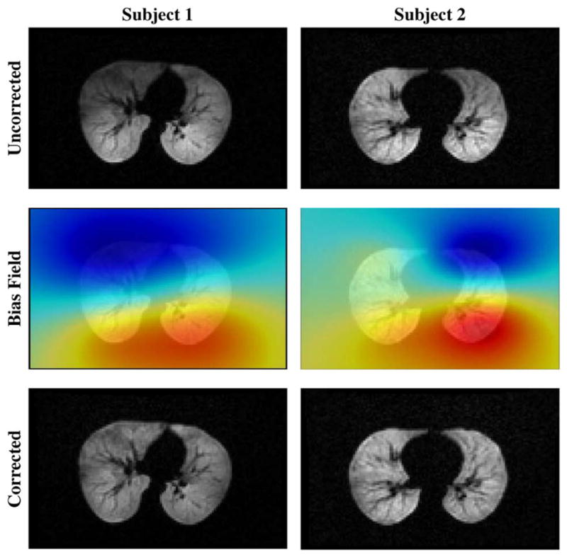
Top row: Axial 3 Hp lung MRI from two subjects evidencing bias field artifacts. Middle row: The calculated bias field. Bottom row: Corrected images.
For purposes of algorithmic comparison, these image data were resampled to (1.6 mm x 1.6 mm x 1.6 mm) using linear interpolation. The following parameters were used for both algorithms: full width at half maximum = 0.15, total number of iterations = 200 (the convergence threshold was set to a very small number to force execution of all 200 iterations), and shrink factor = 4. N3MNI was run on all 156 image data using spline distances of 200 mm, 100, 50, and 25 mm. Similarly N4ITK was run using an initial spline distance of 200 mm where we varied the number of levels from 1 to 4 such that the final spline distances were also 200, 100, 50, and 25 mm. The performance of each run was ranked separately for each algorithm according to coefficient of variation difference between the initial masked region and the corrected masked region [see (27)]. It was found that the best performance achieved by N3MNI was the run of 50 mm (only one image datum of the 156 converged to a nondegenerate solution for the spline distance of 25 mm). The best performance achieved by N4ITK was the run where four multiresolution levels were employed. Performing a pairwise t-test (one-tailed, α = 0.05) on these two sets of results where the null hypothesis is identical means in performance resulted in a rejecting of the null hypothesis with a p value of 10−43 demonstrating superior performance of N4ITK.
C. 9.4T Postmortem Hippocampus Data
Images of five hippocampus samples (three right, two left) were acquired on a 9.4T Varian 31-cm horizontal bore scanner (Varian Inc, Palo Alto, CA) using a 70 mm ID TEM transmit/receive volume coil (Insight Neuroimaging Systems, Worchester, MA) and a multislice spin echo sequence with TR/TE = 5 s/25 ms and 0.2 mm slice thickness. An oblique slice plane was chosen to cover the hippocampus with as few slices as possible (around 130 slices for most images). The phase encode direction was from left to right and the readout direction followed the long axis of the hippocampus. The field of view was typically 60 mm x 90 mm, with matrix size 300 × 300, yielding 3-D images of 0.2 × 0.2 × 0.3 mm3 resolution. Samples were scanned over 12–16 h with 32–44 averages. One sample was scanned at 0.2 × 0.2 × 0.2 mm3 resolution with 225 averages over 63 h. Further details are provided in [23].
For both algorithms, the following parameters were used: full width at half maximum = 0.15, total number of iterations = 200 (the convergence threshold was set to a very small number to force execution of all 200 iterations), and shrink factor = 2. Due to the high held strength, N3MNI was run using a spline distance of 50 mm whereas N4ITK was run using a spline distance of 100 mm at the coarsest resolution level with four total levels for a spline distance of 12.5 mm at the final level. These results are provided in Fig. 7 where 2-D sagittal views of the original image and the corrected and bias field images of the two different algorithms are given. Note the increased locality of the resulting bias field using our proposed algorithm.
Fig. 7.
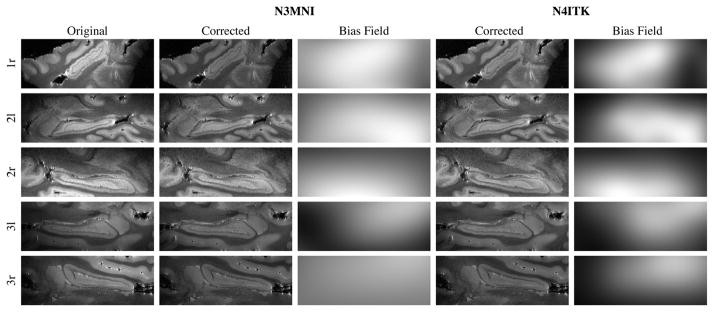
The first column gives 2-D sagittal views of postmortem hippocampi in three subjects (“r” denotes right hippocampus, “l” denotes left hippocampus). The second and third columns give the corrected image using N3MNI and the corresponding bias field whereas the results using N4ITK are provided in columns 4 and 5.
VI. Conclusion
We presented a variant of the well-known N3 algorithm for bias correction of various medical image data. This variation couples a robust B-spline approximation algorithm with a modified optimization strategy which includes a multiresolution option to capture a range of bias modulation. We showcased N4ITK by comparing it with N3MNI using simulated BrainWeb data, hyperpolarized 3He MRI lung data, and postmortem hippocampus data acquired at 9.4T. Furthermore, and of most practical significance, we have made the software publicly available for people to use through the Insight Toolkit of the National Institutes of Health.
Acknowledgments
This work was supported by the National Institute on Aging under Award K25AG027785.
The authors would like to thank Dr. E. E. de Lange and Dr. T. A. Altes at the University of Virginia for providing the hyperpolarized 3He data.
Footnotes
A related issue is the inversion of potentially large, sparse matrices which is computationally demanding for large approximation problems.
Contributor Information
Nicholas J. Tustison, Email: ntustison@wustl.edu, Department of Radiology, University of Pennsylvania, Philadelphia, PA 19140 USA
Brian B. Avants, Email: avants@grasp.cis.upenn.edu, Department of Radiology, University of Pennsylvania, Philadelphia, PA 19103 USA
Philip A. Cook, Email: cookpa@mail.med.upenn.edu, Department of Radiology, University of Pennsylvania, Philadelphia, PA 19103 USA
Yuanjie Zheng, Email: zhengyuanjie@gmail.com, Department of Radiology, University of Pennsylvania, Philadelphia, PA 19103 USA.
Alexander Egan, Email: eganaj@sas.upenn.edu, Department of Radiology, University of Pennsylvania, Philadelphia, PA 19103 USA.
Paul A. Yushkevich, Email: pauly2@grasp.upenn.edu, Department of Radiology, University of Pennsylvania, Philadelphia, PA 19103 USA
James C. Gee, Email: gee@pobox.upenn.edu, Department of Radiology, University of Pennsylvania, Philadelphia, PA 19103 USA
References
- 1.Belaroussi B, Milles J, Carme S, Zhu YM, Benoit-Cattin H. Intensity nonuniformity correction in MRI: Existing methods and their validation. Med Image Anal. 2006 Apr;10(2):234–246. doi: 10.1016/j.media.2005.09.004. [DOI] [PubMed] [Google Scholar]
- 2.Hou Z. A review on MR image intensity inhomogeneity correction. Int J Biomed Imag. 2006;2006:1–11. doi: 10.1155/IJBI/2006/49515. [DOI] [PMC free article] [PubMed] [Google Scholar]
- 3.Vovk U, Pernus F, Likar B. A review of methods for correction of intensity inhomogeneity in MRI. IEEE Trans Med Imag. 2007 Mar;26(3):405–421. doi: 10.1109/TMI.2006.891486. [DOI] [PubMed] [Google Scholar]
- 4.Sled JG, Zijdenbos AP, Evans AC. A nonparametric method for automatic correction of intensity nonuniformity in MRI data. IEEE Trans Med Imag. 1998 Feb;17(1):87–97. doi: 10.1109/42.668698. [DOI] [PubMed] [Google Scholar]
- 5.Arnold JB, Liow JS, Schaper KA, Stern JJ, Sled JG, Shattuck DW, Worth AJ, Cohen MS, Leahy RM, Mazziotta JC, Rottenberg A. Qualitative and quantitative evaluation of six algorithms for correcting intensity nonuniformity effects. Neuroimage. 2001 May;13(5):931–943. doi: 10.1006/nimg.2001.0756. [DOI] [PubMed] [Google Scholar]
- 6.Boyes RG, Gunter JL, Frost C, Janke AL, Yeatman T, Hill DLG, Bernstein MA, Thompson PM, Weiner MW, Schuff N, Alexander G, Killiany RJ, DeCarli C, Jack CR, Fox NC, Study ADNI. Intensity nonuniformity correction using N3 on 3-T scanners with multichannel phased array coils. Neuroimage. 2008 Feb;39(4):1752–1762. doi: 10.1016/j.neuroimage.2007.10.026. [DOI] [PMC free article] [PubMed] [Google Scholar]
- 7.Zheng W, Chee MWL, Zagorodnov V. Improvement of brain segmentation accuracy by optimizing nonuniformity correction using N3. Neuroimage. 2009 Oct;48(1):73–83. doi: 10.1016/j.neuroimage.2009.06.039. [DOI] [PubMed] [Google Scholar]
- 8.Lee S, Wolberg G, Shin SY. Scattered data interpolation with multilevel B-splines. IEEE Trans Vis Comput Graphics. 1997 Jul-Sep;3:228–244. [Google Scholar]
- 9.Tustison NJ, Gee JC. N-d Ck B-spline scattered data approximation. Insight J. 2005:1–13. [Google Scholar]
- 10.Tustison NJ, Gee JC. Generalized n-d Ck B-spline scattered data approximation with confidence values. Proc 3rdInt Workshop Med Imag Augmented Reality. 2006:76–83. [Google Scholar]
- 11.Ibanez L, Schroeder W, Ng L, Cates J. The ITKSoftware Guide. 2. Albany, NY: Kitware; 2005. [Google Scholar]
- 12.Tustison NJ, Gee JC. N4ITK: Nick’s N3 ITK implementation for MRI bias field correction. Insight J. 2009 [Google Scholar]
- 13.Riesenfeld RF. PhD dissertation. Syracuse Univ; Syracuse, NY: 1975. Applications of B-spline approximation to geometric problems of computer-aided design. [Google Scholar]
- 14.Cox MG. The numerical evaluation of B-splines. J Inst Math Appl. 1972;10:134–149. [Google Scholar]
- 15.de Boor C. On calculating with B-splines. J Approx Theory. 1972;6:50–62. [Google Scholar]
- 16.Ma W, Kruth JP. Parameterization of randomly measured points for least squares fitting of B-spline curves and surfaces. Computer-Aided Design. 1995;27:663–675. [Google Scholar]
- 17.Thompson A, Brown J, Kay J, Titterington D. A study of methods of choosing the smoothing parameter in image restoration by regularization. IEEE Trans Pattern Anal Mach Intell. 1991 Apr;13:326–339. [Google Scholar]
- 18.Schoenberg IJ. Spline functions and the problem of graduation. Proc Nat Acad Sci. 1964;52:947–950. doi: 10.1073/pnas.52.4.947. [DOI] [PMC free article] [PubMed] [Google Scholar]
- 19.Tustison NJ, Amini AA. Biventricular myocardial strains via nonrigid registration of anatomical NURBS model corrected. IEEE Trans Med Imag. 2006 Jan;25(1):94–112. doi: 10.1109/TMI.2005.861015. [DOI] [PubMed] [Google Scholar]
- 20.Hjelle O. Approximation of scattered data with multilevel B-splines. Tech Rep, Tech Rep 2001 [Google Scholar]
- 21.Jones CK, Wong EB, Sonka MJ, Fitzpatrick M, editors. Multi-Scale application of the N3 method for intensity correction of MR images. Med Imag 2002: Image Process. 2002;4684:1123–1129. [Google Scholar]
- 22.Manjon JV, Lull JJ, Carbonell-Caballero J, García-Martí G, Martí-Bonmatí L, Robles M. A nonparametric MRI inhomogeneity correction method. Med Image Anal. 2007 Aug;11(4):336–345. doi: 10.1016/j.media.2007.03.001. [DOI] [PubMed] [Google Scholar]
- 23.Yushkevich PA, Avants BB, Pluta J, Das S, Minkoff D, Mechanic-Hamilton D, Glynn S, Pickup S, Liu W, Gee JC, Grossman M, Detre JA. A high-resolution computational atlas of the human hippocampus from postmortem magnetic resonance imaging at 9.4 T. Neuroimage. 2009 Jan;44(2):385–398. doi: 10.1016/j.neuroimage.2008.08.04. [DOI] [PMC free article] [PubMed] [Google Scholar]
- 24.Collins DL, Zijdenbos AP, Kollokian V, Sled JG, Kabani NJ, Holmes CJ, Evans AC. Design and construction of a realistic digital brain phantom. IEEE Trans Med Imag. 1998 Jun;17(3):463–468. doi: 10.1109/42.712135. [DOI] [PubMed] [Google Scholar]
- 25.Aubert-Broche B, Evans AC, Collins L. A new improved version of the realistic digital brain phantom. Neuroimage. 2006 Aug;32(1):138–145. doi: 10.1016/j.neuroimage.2006.03.052. [DOI] [PubMed] [Google Scholar]
- 26.Aubert-Broche B, Griffin M, Pike G, Evans A, Collins D. Twenty new digital brain phantoms for creation of validation image data bases. IEEE Trans Med Imag. 2006 Nov;25(11):1410–1416. doi: 10.1109/TMI.2006.883453. [DOI] [PubMed] [Google Scholar]
- 27.Swift AJ, Wild JM, Fichele S, Woodhouse N, Fleming S, Waterhouse J, Lawson RA, Paley MNJ, Beek EJRV. Emphysematous changes and normal variation in smokers and COPD patients using diffusion 3He MRI. Eur J Radiol. 2005 Jun;54(3):352–358. doi: 10.1016/j.ejrad.2004.08.002. [DOI] [PubMed] [Google Scholar]
- 28.Fichele S, Woodhouse N, Swift AJ, Said Z, Paley MNJ, Kasuboski L, Mills GH, van Beek EJR, Wild JM. MRI of helium-3 gas in healthy lungs: Posture related variations of alveolar size. J Magn Reson Imag. 2004 Aug;20(2):331–335. doi: 10.1002/jmri.20104. [DOI] [PubMed] [Google Scholar]
- 29.Miller GW, Altes TA, Brookeman JR, Lange EED, Mugler JP. Hyperpolarized 3 He lung ventilation imaging with b1-inhomogeneity correction in a single breath-hold scans. MAGMA. 2004 Apr;16(5):218–226. doi: 10.1007/s10334-003-0028-2. [DOI] [PubMed] [Google Scholar]