Correction for spatial averaging in laser speckle contrast analysis

Abstract

Practical laser speckle contrast analysis systems face a problem of spatial averaging of speckles, due to the pixel size in the cameras used. Existing practice is to use a system factor in speckle contrast analysis to account for spatial averaging. The linearity of the system factor correction has not previously been confirmed. The problem of spatial averaging is illustrated using computer simulation of time-integrated dynamic speckle, and the linearity of the correction confirmed using both computer simulation and experimental results. The valid linear correction allows various useful compromises in the system design.

1. Introduction

Laser speckle contrast analysis (LASCA), also known as Laser Speckle Perfusion Imaging (LSPI) has been developed since the late 1970s as a method for measuring and imaging blood flow in capillaries and larger vessels [1,2], as well as the movement of other biological particles in fluids. Tissue is illuminated using an expanded laser beam, and reduced contrast of speckle patterns in the resulting image indicates blood flow. Speckle contrast measurements are susceptible to spatial averaging and other contrast reducing effects, which many researchers have dealt with using a linear system correction factor β [3,4]. We are not aware of any pre-existing justification in the speckle contrast analysis literature for the linearity of this correction, though researchers have investigated similar effects in interferometric speckle measurements [5,6].

In this work we illustrate the effects of spatial averaging in reducing measured speckle contrast, and show that a simple linear correction does recover the true speckle contrast in spatially-averaged results. The same correction is found to apply to the case where speckle contrast is reduced by addition of incoherent background light to the laser illumination. This linear correction is useful as it allows greater latitude for compromise in speckle imaging system design and operation. As some degree of spatial averaging is inevitable in all practical speckle contrast imaging systems, a linear correction also allows inter-system and inter-experiment comparison of speckle contrast measurements.

1.1 Laser speckle perfusion imaging

In a typical laser speckle perfusion imaging application, tissue is illuminated using a laser with an expanded beam and imaged using a video camera. This generates a dynamic speckled image, where the fluctuations of the speckles indicate movement in the multiply-scattered paths that light has travelled through the tissue. The rate of these fluctuations indicates the speed and number of moving scatterers in the tissue, a result confirmed by comparison to laser Doppler experiment and theory [3].

Rather than measure the fluctuations directly, speckle contrast measurements use a finite camera exposure, or a range of exposures, and infer the fluctuation rate and amplitude from the degree of blurring of the speckle pattern at each exposure. This blurring is generally quantified as speckle contrast, defined in the equation:

$$K=\raisebox{1ex}{$\sigma $}\!\left/ \!\raisebox{-1ex}{$\overline{I}$}\right.$$ (1)

where σ is the standard deviation and Ī the mean intensity of the image [7]. K is reduced by the blurring effect of movement in the imaged object. K is typically calculated over small areas of the original speckle image to generate a speckle contrast image and the reduction in K from its maximum value is interpreted as the result of blood flow. Speckle contrast images can be interpreted as they stand as qualitative flow maps, or further processed to yield quantitative flow measurements according to a number of models and analyses [3,4,8]. Any such quantitative application of speckle contrast requires that all the factors influencing the contrast are considered, including the effects of spatial averaging that inevitably occur when using cameras with a finite pixel size and spacing.

A critical adjustable parameter in an imaging laser speckle system is the lens aperture, as it determines the speckle size as described in the equation below, where s is an approximation of the minimum speckle size for an imaging system with magnification M and f-number N working at wavelength λ [9]:

$$s\approx 1.2(1+M)\lambda N$$ (2)

If the speckle size is significantly smaller than the pixel size, the speckle contrast falls as the square root of the number n of coherence regions inside the measurement area, as shown by Goodman [7]:

$$K=1/\sqrt{n}$$ (3)

It is therefore important that the speckle size is at least as large as the pixel size. Many of the earlier speckle imaging systems chose a lens f-number so that the speckle size is approximately equal to the camera chip pixel spacing [10,11]. Kirkpatrick et al. have shown through simulations that this effectively undersamples the speckle pattern, and that the minimum speckle size to avoid undersampling is twice the pixel spacing - a straightforward application of the Nyquist criterion [12]. Their simulations show that when the pixel size equals speckle size the speckle contrast is significantly reduced. This contrast reduction is not caused by sampling points occurring too far apart, as might be implied by the use of the Nyquist theorem, but by spatial averaging of the light across each individual pixel.

2. Spatial averaging and sampling effects

2.1. Simulated static speckle, with spatial averaging

In order to illustrate the effects of spatial averaging and sampling and to test the viability of a correction for errors introduced by spatial averaging, we have repeated simulations developed by Duncan and Kirkpatrick with some variations, using adapted versions of their code [13].

To simulate a single frame of speckle, we start from a zero-filled matrix of size L by L, containing a smaller square area of size L' by L' which contains complex numbers with unity amplitude and randomly distributed phase, on a uniform distribution between 0 and 2π. This smaller area represents the set of random light paths contributing to the speckle pattern, the phases of the complex numbers representing the random phase added to each light path during scattering from tissue. The speckle pattern is generated by taking the two dimensional Fourier transform of the L by L matrix, and multiplying the result by its complex conjugate. A L' by L' subset of the resulting matrix gives a non-repeating speckle image with an exponential intensity distribution matching real fully developed speckle. The minimum speckle size in the pattern is given by the ratio L:L'.

A range of speckle images were developed from an initial synthesized speckle image with different effective speckle sizes relative to the pixel size. The initial image was generated with a minimum speckle size s = 20 pixels, and subsequent images with smaller effective speckle sizes were produced by low-pass filtering using box-car filters with the sizes 1 to 128 pixels, followed by down-sampling, to generate a set of images with effective speckle sizes between 20 and 0.16 pixels. This procedure simulates the effect of increasing the lens aperture in a real speckle system and thus reducing the speckle size relative to the camera pixels. The size of all the simulated speckle images was 200 by 200 pixels.

Figure 1 shows the results of this procedure. The speckle contrast rises continuously with increasing speckle size. The annotated points in Fig. 1 indicate the two speckle size criteria introduced above. At the commonly used speckle size of one pixel, the speckle contrast is approximately 0.7. At a speckle size of two pixels, corresponding to the Nyquist criterion, the speckle contrast is approximately 0.9. Despite meeting the Nyquist criterion for sufficient sampling, there is still a definite reduction in contrast at a speckle size of 2 pixels due to the spatial averaging effect of the finite pixels.

Fig. 1.

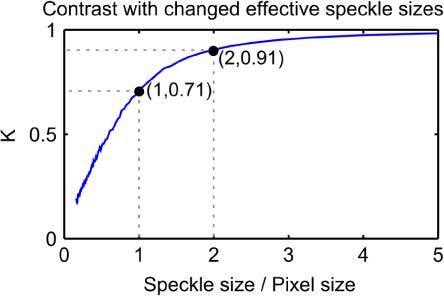
Speckle contrast with changing speckle size as a ratio of pixel size, using simulated speckle data. Dashed lines and annotated points refer to speckle size criteria often described in the literature.

2.2. Calculation region size and sampling

The contrast values above were calculated by taking standard deviation and mean over the whole 200 by 200 pixel speckle image. However, in speckle imaging the contrast is usually calculated over relatively small regions of the raw image. As the speckle contrast is a statistical measurement, the calculation area needs a sufficient number of pixels that the standard deviation and mean of the sample are meaningful. The calculation region, generally a square, needs to be a multiple of the minimum speckle size and has often been set at 5 x 5 or 7 x 7 pixels [14,15].

In order to quantify the effect of changing region size, the speckle calculation region was varied in the range 2 x 2 to 200 x 200 pixels and the contrast re-calculated. The effective speckle size was held at its original value of 20 pixels for these calculations. For each region size, the contrast was calculated for regions covering the whole simulated speckle image and the mean of the contrast found. The results are plotted in Fig. 2 .

Fig. 2.

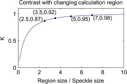
Change in measured speckle contrast with varying square contrast calculation region, using simulated speckle data.

The annotated points in Fig. 2 indicate the effective region sizes generated by combinations of common speckle size and region size criteria. The two effects of speckle to pixel size and region size are considered independently here, but will clearly interact in practice – the calculation region will produce a further reduction in measured speckle contrast if it is not sufficiently large.

3. Maximum and minimum contrast K_max and K₀, and correction factor β

As there are practical limits to achieving the perfect statistical situation of very large speckles, many applications of laser speckle for quantitative measurements use an analysis that recognizes that the maximum achievable contrast K_max will be reduced by spatial averaging and other experimental factors. Researchers in this field have used a linear system correction factor β = 1/K_max to account for a maximum achievable speckle contrast K_max less than 1 [3,4]. The measured speckle contrast is multiplied by this linear factor in order to estimate the true speckle contrast during data processing.

We have also found a minimum contrast parameter K₀ useful in situations where there is a static component to the dynamic speckle pattern. This can occur when there is a static layer of scatterers overlaying tissue containing moving scatterers; for example, in imaging blood flow through the thickly calloused skin of the sole of the foot. K₀ represents the minimum contrast achievable at camera exposures sufficiently long that all of the dynamic contributions to the speckle pattern are blurred – thus, it represents the proportion in intensity of the speckle pattern contributed by totally static paths.

3.1. Simulated speckle with temporal blurring and a static component

In order to test the validity of a linear β correction, the effect of spatial averaging on the measured contrast of speckle images captured at a range of exposures was simulated in MATLAB. This simulation uses a technique we have previously described [3], based on Duncan and Kirkpatrick's work [13], to generate speckle images with temporal blurring consistent with real speckle images captured in tissue at a range of exposures. In this technique the instantaneous speckle intensity is generated as described above, by a Fourier transform of a generating matrix.

To generate a series of frames with a small inter-frame change in the speckle pattern, we repeatedly add a small randomly distributed phase to the phases in the L' by L' square in the generating matrix and recalculate the speckle pattern. In previous work we have added this phase step to every element in the L' by L' square, resulting in a totally dynamic speckle pattern [3]. In this work, we hold a proportion of the elements static, so that the simulated speckle images have both a dynamic and a static component. The static elements are distributed randomly, with a uniform distribution throughout the L' by L' matrix in order that they will have approximately the same maximum separation, and the static and dynamic components of the speckle pattern will have the same minimum speckle size s. The effects of temporal blurring are simulated by taking sums of series of adjacent frames – in effect, integrating the fluctuating intensity in the same way as a camera with a finite exposure time. At long exposures, we find that the minimum contrast K₀ approaches the proportion of static scatterers in the generating matrix.

3.2. Applying β correction to spatially-averaged speckle

An original set of 256 images was generated with simulated exposures T from 0 to 255 arbitrary units and the static proportion of the speckle generating matrix at 0.4. These images have a minimum speckle size s of 20 pixels and contrast K ranging between the ideal value of 1, for exposure of 0 units, and 0.41 for the longest exposure of 255 units as K approaches the predicted K₀ of 0.4. Spatial averaging was applied to the original images, using the same filtering and sub-sampling procedure as described above to simulate imaging the dynamic speckle with a range of lens apertures, and hence a range of speckle sizes. The results are plotted in Fig. 3 .

Fig. 3.

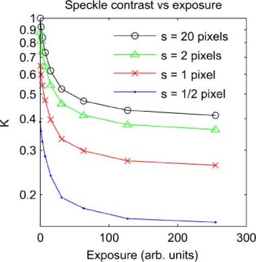
Simulation results for apparent contrast of dynamic speckle measured at a range of exposures, and with a range of speckle sizes.

Each curve in Fig. 3 represents the speckle contrast that will be measured at a range of camera exposures, given a particular speckle size s relative to the camera pixels. For the s = 20 curve there is no effect of spatial averaging – the contrast falls from an initial value of 1 with increasing camera exposure, approaching the static contrast value of K₀ = 0.4. The other curves show the effect of introducing some spatial averaging – the speckle contrast at every exposure is reduced. We can define a K_max for each curve as the value of contrast that will be measured given no temporal blurring. In the case of these simulations, that is the contrast at T = 0. Normalizing each curve by dividing by its respective K_max produces Fig. 4 .

Fig. 4.

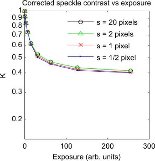
Simulated speckle contrast measured at a range of exposures, with β correction applied.

The normalization by β = 1/K_max successfully recovers the true speckle contrast, indicating that this linear correction is valid in this case.

3.3. Applying β correction to speckle with background light addition

The maximum achievable speckle contrast can also be reduced in some situations by the addition of a background light level to the speckle pattern, as might occur when an incoherent background light source adds to the laser illumination. This situation was simulated by adding a constant background value to speckle images with s = 20. For background level b and original image intensities I_o the new image intensities are I = (1-b)I_o + b. The background level b was varied in steps from 0 to 0.4, reducing Kmax from 1 to 0.17. Figure 5 shows the uncorrected speckle contrast at a range of exposures for each background level, and Fig. 6 shows the corrected curves. Again, a simple normalization by β = 1/K_max recovers the true speckle contrast.

Fig. 5.

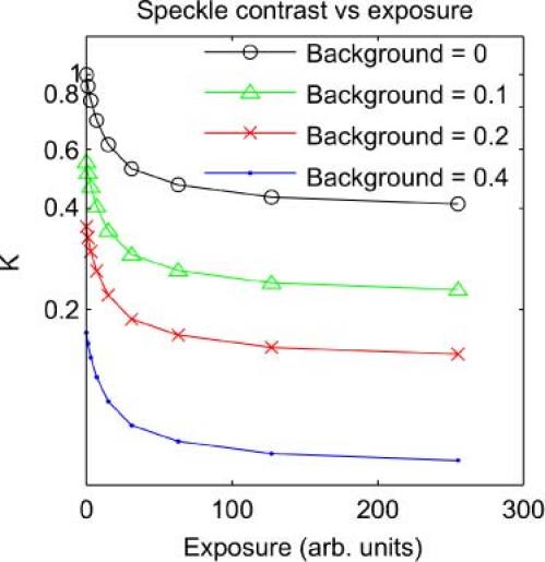
Simulated speckle contrast at a range of exposures, with some contrast reduction due to background light addition.

Fig. 6.

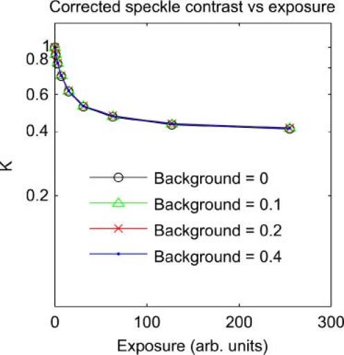
Simulated speckle contrast at a range of exposures, contrast reduction due to background addition corrected using B = 1/ K_max factor.

3.4. Experimental confirmation of β linearity

The linear β = 1/ K_max correction for reduced maximum achievable speckle contrast was also tested experimentally, using speckle contrast measured on both skin and a simple phantom at a range of camera exposures, with the maximum achievable contrast K_max reduced by spatial averaging. Speckle images were made using a conventional speckle contrast imaging system, consisting of a Sony CCD camera with polarizing filter and a 12-36 mm varifocal lens, and a 658 nm, 30 mW laser diode module from Ondax [16]. These modules are volume Bragg grating stabilized and have a stable and long coherence length. The targets for these tests were the skin of the palm, and a phantom consisting of a container of milk, providing a Brownian motion source, covered with a thin static scattering layer made from silicone and alumina powder [17].

Contrast vs. exposure curves at each degree of spatial averaging were produced. The degree of spatial averaging was progressively increased by opening the lens aperture until contrast at a particular exposure was significantly reduced, then repeating the contrast measurements over the exposure range. As the varifocal lens used has no marked f-stops and the speckle size is comparable to the pixel size, precluding a determination of s by autocorrelation, the value of speckle size s for these curves is not easily obtained. K_max values used for correction were obtained by measuring the speckle contrast on a static multiply-scattering target, consisting of a block of the silicone/alumina mixture used above. All of the data recorded shows some degree of spatial averaging, with K_max ranging from 0.83 to 0.32.

The results of these experiments are plotted in Fig. 7 – the uncorrected results in the upper two subplots, and corrected versions of these results in the lower two subplots.

Fig. 7.

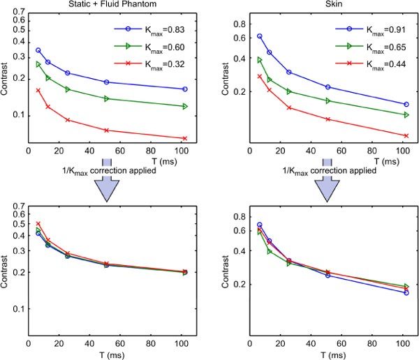
Results of experimental testing of β = 1/K_max correction for spatial averaging.

4. Conclusions

A linear correction for reduced speckle contrast due to spatial averaging or background light addition is valid. This is confirmed by both simulation and experiments for dermal perfusion measurements and a measurements on a phantom combining static and dynamic scattering.

The correction value β = 1/K_max can be measured using a static target as we have done, or could be found by extrapolating a K vs. T curve to T = 0 or inferred from the aperture and pixel size of the camera.

The validity of the correction has significant practical implications. As all practical system setups will introduce a degree of spatial averaging, such a correction will always be required for any comparison of speckle contrast or related parameters between measurements under different experimental conditions. Such inter-system or inter-experiment comparison is necessary in many clinical and research situations.

As the speckle size is proportional to the f-number of the lens, it follows that the mean intensity at the sensor is inversely proportional to the square of the speckle size. Reducing the aperture in order to reduce spatial averaging can significantly reduce the light available at the sensor due to this inverse square relationship. Given that the camera exposure will generally be set at a pre-defined value or range of values the linear β correction allows a trade-off between light levels and spatial averaging in the selection of an optimum working aperture.

In addition, the spatial resolution of a digital camera is further reduced due to the speckle calculation region size which must be a multiple of the speckle size, as shown in Fig. 2. Increasing the speckle size to eliminate spatial averaging requires a larger calculation region, reducing the final spatial resolution of the system.

Both the light reduction and spatial resolution effects can be reduced by a compromise choice of aperture and speckle size which allows a level of spatial averaging, subsequently correcting for the reduced speckle contrast. The linear β correction for spatial averaging makes this compromise possible.