

Abstract
Chromatin immunoprecipitation (ChIP) coupled with genome tiling array hybridization (ChIP-chip) and ChIP followed by massively parallel sequencing (ChIP-seq) are high throughput approaches to profile genome-wide protein-DNA interactions. Both technologies are increasingly used to study transcription factor binding sites and chromatin modifications. CisGenome is an integrated software system for analyzing ChIP-chip and ChIP-seq data. This unit describes basic functions of CisGenome and how to use them to find genomic regions with protein-DNA interactions, visualize binding signals, associate binding regions with nearby genes, search for novel transcription factor binding motifs, and map existing DNA sequence motifs to user-supplied genomic regions to define their exact locations.
Keywords: transcription factor, chromatin immunoprecipitation, tiling array, next generation sequencing, motif, gene regulation
INTRODUCTION
Chromatin immunoprecipitation (ChIP) coupled with genome tiling array hybridization (ChIP-chip) (Ren et al., 2000; Cawley et al., 2004) and ChIP followed by massively parallel sequencing (ChIP-seq) (Barski et al., 2007; Johnson et al., 2007; Mikkelsen et al., 2007; Robertson et al., 2007) are powerful technologies for mapping transcription factor binding sites and chromatin modifications. A typical ChIP-chip or ChIP-seq experiment generates tens of millions of data points. Extracting useful information from the huge amount of data is a significant computational challenge. CisGenome (Ji et al., 2008) is an integrated software system to help researchers to cope with this challenge. This software contains a wide range of functionalities including (1) identification of protein-DNA binding regions from ChIP-chip data (also known as “peak calling”), (2) ChIP-seq peak calling, (3) data visualization, (4) association of peaks with nearby genes, (5) retrieving DNA sequences, (6) novel transcription factor binding motif discovery, and (7) mapping existing motifs to protein-DNA binding regions (Figure 2.13.1). This unit introduces how a typical user can use these functions to perform basic ChIP-chip and ChIP-seq data analyses.
Figure 2.13.1.

Overview of the CisGenome basic data analysis pipeline.
ChIP-chip and ChIP-seq data analyses typically begin with detection of genomic regions that contain the protein-DNA interactions of interest. Usually, this involves processing raw microarray or sequence data in order to remove technological biases and distinguish bona fide biological signals from random noises. The signals often stand out as some kind of enrichment, such as increased probe intensities in ChIP-chip or elevated sequence read count in ChIP-seq. In this unit, detection of these enrichment signals is also referred to as “peak calling”. After obtaining a list of putative protein-DNA binding regions, one can proceed to visually examine the enrichment signals in these regions, with gene annotations (e.g. starts and ends of exons and introns) and probe signals or sequence read counts displayed side by side. Visualization is not only a useful way to identify potential artifacts in the experimental data, but also an important first step to make new discoveries. Once the visual examination confirms the data quality, one can then annotate protein-DNA interactions by nearby genes. Genes pulled out in this way can be used to shed light on functions of transcription factors or chromatin marks through subsequent analyses of gene ontology (The Gene Ontology Consortium, 2000; see Unit 7.2) or cross-referencing with gene expression data. For many transcription factors the DNA sequences in the binding regions provide an opportunity to discover the specific DNA sequence patterns (also called “motifs”) recognized by the transcription factors, if such patterns are not already known. It is believed that transcription factor binding motifs are part of the mysterious and highly complex genetic codes written in the genome to dictate when, where and at what level genes should be expressed. Understanding these codes will greatly help us to understand mechanisms behind gene regulation and diseases. There are also a large number of transcription factors for which the DNA binding motifs have already been characterized. For both known and new motifs, it is useful to map them to protein-DNA binding regions to identify their exact locations. These loci can serve as candidates for subsequent experimental validation, such as knock-out or transgenic experiments.
Following the natural order of data analyses, this unit is organized as follows (Figure 2.13.1). First, we will introduce how to use CisGenome to call peaks from ChIP-chip data generated by using Affymetrix genome tiling arrays (Basic Protocol 1). Next, we will present protocols to visualize enrichment signals (Basic Protocol 2), associate peaks with genes (Basic Protocol 3), retrieve DNA sequences (Basic Protocol 4), discover novel transcription factor binding motifs (Basic Protocol 5), and mapping motifs to genomic regions (Basic Protocol 6). Collectively, these protocols can be assembled into a basic analysis pipeline for processing Affymetrix ChIP-chip data. Peak calling for non-Affymetrix ChIP-chip data will be introduced in Basic Protocol 7, and ChIP-seq peak calling will be introduced in Basic Protocols 8 and 9. Once peak calling is done, subsequent analyses can be performed in the same way as described in Basic Protocols 2-6. Therefore, by replacing Basic Protocol 1 by Basic Protocols 7-9, one can easily construct analysis pipelines for non-Affymetrix ChIP-chip and ChIP-seq data. In addition to the basic protocols we also provide two support protocols. Support Protocol 1 introduces how to install CisGenome. Support Protocol 2 introduces how to install genome databases required by many analysis functions of CisGenome.
BASIC PROTOCOL 1
CHIP-CHIP PEAK CALLING FOR AFFYMETRIX TILING ARRAY DATA
This section introduces how to use CisGenome to detect protein-DNA binding regions from an Affymetrix tiling array experiment. A tiling array is a microarray that contains probes to interrogate the whole genome or targeted genomic regions. ChIP-chip experiments are usually carried out by hybridizing ChIP and control DNA samples to tiling arrays. Affymetrix tiling arrays are one of the most popular tiling array platforms currently in use.
A typical Affymetrix tiling array experiment generates multiple CEL files. These files contain raw probe intensities stored in a standard format defined by Affymetrix. Often, data in these files are saved in a binary format to reduce storage space and facilitate efficient data retrieval. This means users may not be able to read the file in a human interpretable way using a text editor.
For each tiling array platform, Affymetrix also provides a library of BPMAP file(s) that contains the array design information. The library may contain one or more BPMAP files which specify how probes in the array(s) are mapped to the genome. The BPMAP files also have a binary format defined by Affymetrix.
In CisGenome, analysis of Affymetrix ChIP-chip data consists of three steps, namely, loading data, sample normalization, and peak calling. We will use a sample data set to illustrate this procedure. The sample data are produced in a ChIP-chip experiment for studying mouse transcription factor Gli3. The data were generated using Affymetrix Mouse Tiling 2.0R array set which contains seven chips in total to cover the whole mouse genome. The BPMAP library contains seven BPMAP files, one for each chip. In the experiment, three ChIP samples and three control samples were profiled. Each sample was hybridized to all seven chips and produced seven CEL files. In total, there are 42 CEL files and 7 BPMAP files. The data can be downloaded from http://www.biostat.jhsph.edu/~hji/cisgenome/index_files/basicprotocol.htm.
Necessary Resources
Hardware
A personal computer (PC) equipped with Windows operating system (OS)
Software
CisGenome (see Support Protocol 1 for installation guide)
Files
CEL files that contain raw tiling array data
BPMAP files that contain the array design information. The BPMAP files can be downloaded from http://www.biostat.jhsph.edu/~hji/cisgenome/index_files/download.htm or http://www.affymetrix.com/.
Load Data
Enter the CisGenome installation folder. Start CisGenome by double-clicking CisGenome.exe.
Click the menu “File > Load Data > Tiling Array Dataset > Import from Affymetrix CEL+BPMAP” (Figure 2.13.2).
- A wizard dialog will appear (Figure 2.13.3a). In this dialog, set parameters as follows:
- Specify a name for the data set (e.g. GliData).
- Click the button highlighted by circle 1.1. In the dialog that jumps out, choose the folder that contains the BPMAP files (circle 1.2) and then click “OK”.
- Now all BPMAP files in the selected folder will be listed in the box on the left-hand side named “Available BPMAP” (Figure 2.13.3b). Select the BPMAP files corresponding to the ChIP-chip data. Click “Add” to move them to the box on the right-hand side titled “BPMAP used in the Project”. For the Gli example, all seven BPMAP files need to be added to the project.
- Use “Move Up” and “Move Down” buttons to adjust the order of BPMAP files (Figure 2.13.3b).
- Click “Next” on the bottom (Figure 2.13.3b).
- A new wizard page will appear (Figure 2.13.4a). Set parameters in this new page as follows:
- Click the button in circle 1.3 (Figure 2.13.4a). In the dialog that appears, choose the folder that contains the CEL files (Figure 2.13.4a, circle 1.4) and then click “OK”.
- Now all CEL files in the selected folder should be listed in the box named “Available Arrays” on the left (Figure 2.13.4b). Click “Create New Sample” (Figure 2.13.4b, circle 1.5) to add a sample to the data set. Provide a sample name in the “Sample ID” box (e.g. use “IP1” for ChIP sample 1, and use “CT3” for Input control sample 3, etc.). Provide a group identifier for the sample in the “Group ID” box (Figure 2.13.4b, circle 1.6). For example, set Group ID = 1 if the sample is a ChIP sample, and set Group ID = 2 if it is a control sample.If the group identifiers are defined in this way, then the expression “1>2” in subsequent analyses will have the meaning that “the mean probe intensity in the ChIP samples is bigger than the mean probe intensity in the control samples”.
- For the newly created sample, find all related CEL files. Select them in the “Available Arrays” box, and click “Add” to move them to the box titled “Arrays in the Sample” (Figure 2.13.4b, circle 1.7).
- Use “Move Up” and “Move Down” buttons to adjust the order of CEL files in the sample so that they match with the corresponding BPMAP files (Figure 2.13.4b, circle 1.8).
- Repeat steps 4b – 4d to add all ChIP and control samples to the data set.
- Click the “Finish” button on the bottom (Figure 2.13.4b).
Check the “Project Explorer” window in the CisGenome GUI (Figure 2.13.5). Under the section titled “Tiling Array Datasets”, a new data set should have been created. If you double-click a CEL file (e.g. Figure 2.13.5, circle 1.9), a CisGenome Browser window should appear.
Figure 2.13.2.
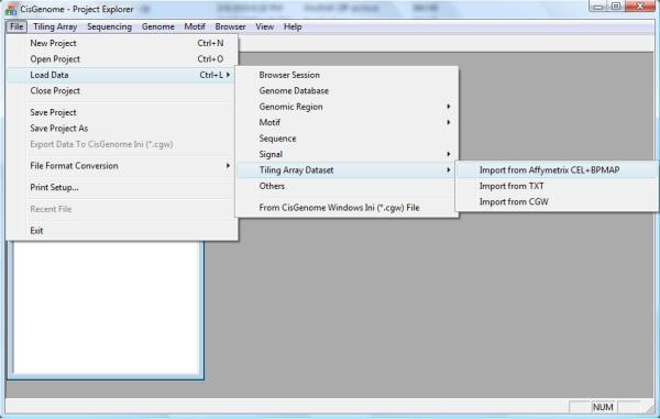
The CisGenome graphic user interface (GUI) and menu system. The menu for creating an Affymetrix tiling array data set is shown as an example.
Figure 2.13.3.

The dialog for adding BPMAP files to an Affymetrix ChIP-chip data set.
Figure 2.13.4.

The dialog for adding CEL files to an Affymetrix ChIP-chip data set.
Figure 2.13.5.

The newly created tiling array data set shown in the CisGenome Project Explorer. Double-clicking a CEL file will open a CisGenome Browser window displaying a heat map of the array image.
The window displays the heat map of the raw image of the selected array (Figure 2.13.5). Once you see the heat map, it suggests that the data has been loaded successfully.
Normalize Samples
-
6.
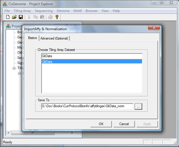
Click the menu “Tiling Array > Normalization > Quantile (CEL+BPMAP)”.
-
7.
In the configuration dialog that jumps out (Figure 2.13.6), specify the tiling array data set (e.g. GliData) to be normalized, and choose a folder and file header (e.g. GliData_norm) to export the normalized array intensities. Click “OK”.
-
8.
The program will start to run. After it is done, a new data set containing the normalized data will be added to Project Explorer under the “Tiling Array Datasets” section (Figure 2.13.7, circle 1.10).
Figure 2.13.6.
The dialog for normalizing an Affymetrix tiling array data set.
Figure 2.13.7.
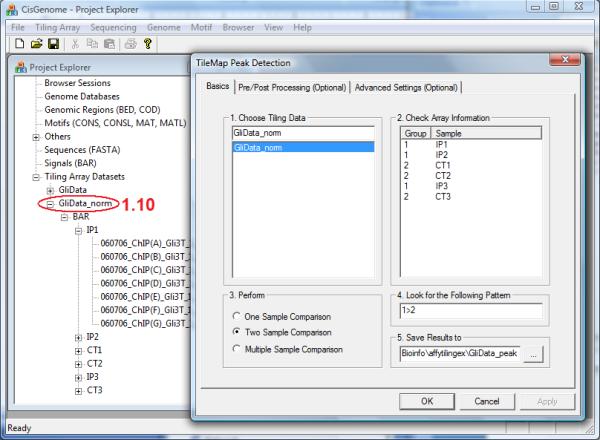
ChIP-chip peak calling. Before peak detection, a normalized tiling array data set (circle 1.10) needs to be available in the Project Explorer, and one needs to provide several basic peak calling parameters in a dialog.
Call Peaks
-
9.
Click the menu “Tiling Array > Peak Detection (TileMap)”.
-
10.In the dialog that jumps out (Figure 2.13.7), provide the following parameters:
- Choose a normalized tiling array data set to analyze (e.g. GliData_norm).
- Choose an analysis type. Use “Two Sample Comparison” if the data contain samples from two experimental conditions (e.g. ChIP vs. control). Use “Multiple Sample Comparison” if the data contain samples from more than two experimental conditions (e.g. ChIP, Input control, and IgG control). “One Sample Comparison” is usually used for non-Affymetrix tiling array data (see Basic Protocol 7).
- Specify a pattern to look for. In a two sample comparison, suppose Group ID = 1 for ChIP samples, and Group ID = 2 for control samples, then the pattern to look for is 1>2. This pattern means that we are trying to find genomic regions where the probe intensities in group 1 (i.e. ChIP samples) are bigger than the probe intensities in group 2 (i.e. control samples). In a multiple sample comparison, the pattern can be specified as a combination of pairwise comparisons such as (1>2 & 1>3), where “&” means AND.
- Specify a folder and a file header to save the results.
- (Optional) Specify parameters in the “Pre/Post Processing” and “Advanced Settings” tabs. The configurable parameters are listed in Table 2.13.1.
- Click “OK”.
-
11.The peak detection program will start to run. After it finishes, the detected peaks will be saved in a COD file named “[file header]_all.cod”, in which [file header] is the file header specified in step 10d. A COD file is a tab-delimited text file with five required columns to describe genomic regions (Figure 2.13.8). The COD file produced by ChIP-chip peak calling will be added to the “Genomic Regions (BED, COD)” section in the Project Explorer (Figure 2.13.8, circle 1.11). It will also be opened and displayed in a window (Figure 2.13.8). In the “Signals” section of the Project Explorer, several BAR files (named as *.bar) will be added as well (Figure 2.13.8, circle 1.12).The first five columns are required. They are (i) a numerical or string identifier, (ii) chromosome, (iii) start coordinate, (iv) end coordinate, and (v) strand. In a COD file, additional columns are allowed after the first five to annotate regions. See section on Guidelines for Understanding Results to learn more about the COD file produced by CisGenome ChIP-chip peak calling. A COD file can be opened and edited by any text editor (e.g. Notepad and EXCEL). The BAR file format is a binary format defined by Affymetrix. The BAR files produced by CisGenome contain probe-level enrichment signals which can be used for subsequent visualization.
-
12.
After the analysis, one can save the project using the menu “File > Save Project” or “File > Save Project As”. Save the project to a file named [project title].cgw (e.g. GliData.cgw). In the future, use the menu “File > Open Project” to load the project back whenever needed.
Table 2.13.1.
Optional parameters for ChlP-chip peak calling
| Parameters and Description |
|---|
| 1. Mask outlier/masked data points in the raw data: if yes, the outlier and masked probes in the original CEL file will not be used in peak detection. |
| 2. Truncation lower bound (TLB): a numerical value. If it is equal to x, then all normalized probe intensities smaller than x will be truncated to x before peak calling. |
| 3. Truncation upper bound (TUB): a numerical value. If it is equal to x, then all normalized probe intensities bigger than x will be truncated to x before peak calling. |
| 4. Transform: before peak calling, the truncated probe intensities can be transformed by log2, logit or inverse logit function. Choose “None” if no transformation is needed. |
| 5. Post processing: one can choose to merge two neighboring peaks if the gap between the two peaks <= x bp and the number of probes below the peak calling cutoff between the two peaks <= y. |
| 6. Post filtering: one can choose to not report a peak if the peak length < x bp or the peak does not contain at least y continuous probes whose enrichment signals are above the peak calling cutoff. Both x and y are integers. |
| 7. Region Summary Method: choose to use TileMap moving average (MA) or Hidden Markov Model (HMM) to call peaks. The default is MA. |
| 8. MA settings: If MA is chosen in 7, provide half window size x and y, and a peak calling cutoff z. For each probe, the MA algorithm uses all probes within y bps and separated from the probe in question by no more than x-1 other probes to compute enrichment signals. If the signal is bigger than z, the probe will be selected to construct peaks. |
| 9. HMM settings: If HMM is chosen in 7, provide the expected peak length x (i.e. how many probes are expected to be covered by an average peak) and the peak cutoff y. The HMM computes a posterior probability for each probe being in a peak. Probes with a posterior probability above y will be used to construct peaks. |
| 10. Method to compute false discovery rate (FDR). Choose from “Left tail”, “UMS”, “Permutation” and “No FDR”. “Left tail” works for two sample comparisons. It flips the ChIP and control sample labels, and detects peaks after the label swap. The FDR is estimated by the ratio [No. of peaks detected after the label swap] / [No. of peaks detected before the label swap]. “UMS” uses the unbalance mixture subtraction method introduced in Ji and Wong (2005) to estimate FDR. “Permutation” works by permuting sample labels and detects peaks afterwards. The FDR is estimated by the ratio [No. of peaks detected after the label permutation] / [No. of peaks detected before the label swap]. “UMS” and “Permutation” can work for multiple sample comparisons. “No FDR” will skip FDR computation. |
| 11. UMS settings, permutation settings, and variance assumptions: These parameters are usually set automatically. Manually setting them requires deep understanding of the TileMap algorithm. Users are referred to Ji and Wong (2005) if they want to learn how to set these parameters manually. |
Figure 2.13.8.
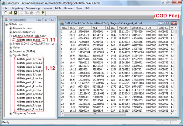
ChIP-chip peak calling results. Peaks are summarized in a COD file shown in the right window. A number of BAR files are also created to store enrichment signals. Both the COD file and the BAR files are added to the Project Explorer on the left.
BASIC PROTOCOL 2
VISUALIZATION
CisGenome provides a light-weight browser which can be used to visualize enrichment signals (e.g. probe intensities in ChIP-chip, or read counts in ChIP-seq) along the genome. This browser runs locally on the user's computer and does not require one to have access to the Internet. This section introduces how to use CisGenome Browser to visualize the data.
An Alternative Way to Display the Data
The procedure described below allows one to create a browser session manually. In fact, if the ChIP-chip and ChIP-seq peak calling is performed within CisGenome GUI, a browser session will be automatically created. In Figure 2.13.8, by choosing a peak in the COD file and double-clicking the first column of the peak, one will be directed to the browser session in which data within the peak are displayed. If the genome database has been loaded into CisGenome GUI before peak calling, then the browser will also display the gene annotation, conservation and DNA sequence tracks automatically.
Necessary Resources
Hardware
A PC equipped with Windows OS
Software
CisGenome (see Support Protocol 1)
A web browser (e.g. Internet Explorer)
Files
BAR files created by CisGenome peak detection (see Basic Protocols 1, 7, 8, 9)
A genome database for the species of interest (see Support Protocol 2)
Visualize Data
Start CisGenome. Locate a black CGB icon on the bottom right corner on the desktop (Figure 2.13.9a, circle 2.1). This is a shortcut icon for CisGenome Browser.
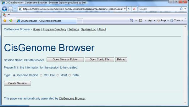
Double-click the CGB icon to start CisGenome Browser (Figure 2.13.9b).
- Before visualizing the data, one has to create a CisGenome Browser session as follows.
- In the browser homepage, provide a session name, for example, “GliDataBrowser” (Figure 2.13.9b). Click “Load or create a session”.
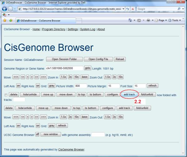
- A new page will appear to ask you to choose a session type (Figure 2.13.10). Choose “Genome Region” and then click “Create Session”. A new empty browser session will be created (Figure 2.13.11).
- In a browser session, one can add data tracks for visualization. Follow the steps below to add a track for displaying enrichment signals in a BAR file.
- Click the “add track” button (Figure 2.13.11, circle 2.2).
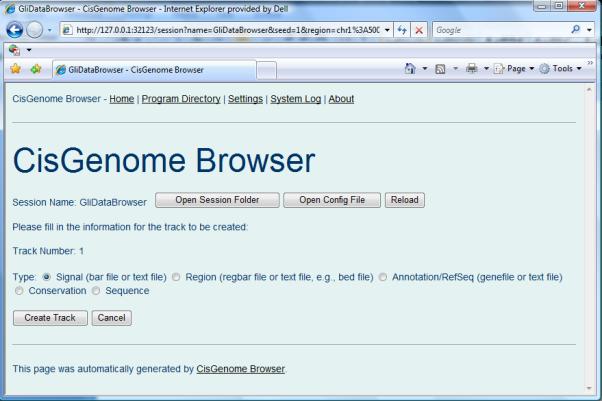
- A new page will appear to ask for track type (Figure 2.13.12). Choose “Signal (bar file or text file)” and then click “Create Track”.
- In the track configuration page that appears, use the “Browse” button to find a BAR file to display (Figure 2.13.13, circle 2.3).
For example, choose the file “GliData_peak_7.fc.bar” created by the analysis of the Gli data in Basic Protocol 1. This file contains log2 fold changes between ChIP and control samples for all probes in array 7 of the Affymetrix Mouse Tiling 2.0R array set. Click the “Update Track” button on the bottom of the page (Figure 2.13.13, circle 2.4). - Similar to adding a track for displaying enrichment signals, one can also add tracks for displaying gene annotations, cross-species conservation scores, and DNA sequences. Follow the steps below to add these tracks:
- Follow Support Protocol 2 (steps 1-3) to download and install the relevant genome database.
- Click the “add track” button in Figure 2.13.11.
- In the browser page for choosing track type (Figure 2.13.12), choose one of the following:
- “Annotation/RefSeq (genefile or text file)” for adding a gene annotation track;
- “Conservation” for adding a cross-species conservation score track;
- “Sequence” for adding a DNA sequence track.
- Now a page similar to Figure 2.13.13 will appear to ask you to choose a file that contains gene annotations, conservation scores, or DNA sequences. Choose the following files:
- For gene annotation: enter the folder where the genome database is installed. Choose the file named “[assembly].genefile” (e.g. mm8.genefile) under the “genefile” subfolder.
- For conservation: enter the folder where the genome database is installed. Enter the “conservation” subfolder. Enter the “phastcons” subfolder which contain phastCons conservation scores (Siepel et al., 2005). Choose any file with a *.cs suffix.
- For DNA sequence: enter the folder where the genome database is installed. Choose any file with a *.sq suffix.
Figure 2.13.9.
CisGenome Browser. (A) The shortcut icon for the browser. (B) The first page of the browser.
Figure 2.13.10.
The browser page for choosing browser session type.
Figure 2.13.11.
An empty browser session newly created.
Figure 2.13.12.
The browser page for choosing data track type.
Figure 2.13.13.

The track configuration page in CisGenome Browser.
After the file is chosen, click the “Update Track” button.
-
6.
Repeat steps 4 and/or 5 to add all data you want to display. The browser will now show all tracks you have added in one page (Figure 2.13.14). Type coordinates of a genomic region (e.g. chr13:63775120-63775698) or a gene name in the “Genome Region or Gene Name” box and click “goto” (Figure 2.13.14, circle 2.5). You will be directed to the genomic region or the gene you have chosen.
-
7.Adjust the display.
- One can zoom in, zoom out, move left or right by clicking the relevant buttons (Figure 2.13.14, circle 2.6).Note that the DNA sequences will only be displayed when the browser is zoomed in sufficiently.
- One can adjust features of the plotting area and then click the “refresh” button to let them take effect (Figure 2.13.14, circle 2.7).
- One can delete or adjust the order of tracks by selecting one or more tracks (Figure 2.13.14, circle 2.8) and then clicking the “delete”, “move up”, “move down”, “to top” or “to bottom” buttons (Figure 2.13.14, circle 2.9).
- One can change the display style for one or more tracks by selecting the track(s) and then clicking the “configure” button (Figure 2.13.14, circle 2.10). A configuration page similar to Figure 2.13.13 will appear to help you choose a variety of parameters including, for instance, the color to display the data, track height, and display range (i.e. the minimal and maximal data values allowed to be shown in the track. Values beyond this range will be truncated before display). Meanings of the parameters in this page are self-evident.
Figure 2.13.14.
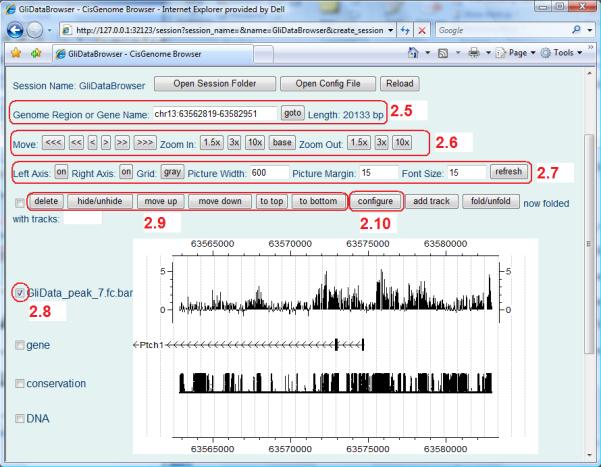
CisGenome Browser showing different types of data. Tools to adjust the display styles are highlighted.
BASIC PROTOCOL 3
PEAK-GENE ASSOCIATION
This section introduces how to annotate peaks with nearby genes. The steps described below retrieve the closest gene of each peak. One can use the menu “Genome > Annotate with ... > Neighboring Genes” and follow a similar procedure to retrieve multiple genes instead of the closest one in the peak neighborhood.
Necessary Resources
Hardware
A PC equipped with Windows OS
Software
CisGenome (see Support Protocol 1)
Files
A peak list stored in a COD file (see Figure 2.13.8). Such a file is usually created by CisGenome peak calling (see Basic Protocols 1, 7, 8, 9).
A genome database for the species of interest (see Support Protocol 2)
Annotate Peaks with Nearby Genes
- Load the genome database into CisGenome GUI (see Support Protocol 2).For example, to analyze the peak generated by the Gli data in Basic Protocol 1, load the mouse mm8 database.
Click the menu “Genome > Annotate with ... > Closest Gene”.
In the dialog that appears (Figure 2.13.15a), choose the peak list (COD file) you want to analyze, choose the corresponding genome database, and specify a file to save the results.
- (Optional) In the same dialog, choose a distance type. This program will extract the closest gene for each and every peak. The closeness is determined by the distance between a peak and its neighboring genes. There are six possible ways to define the distance d between a peak and a gene.
- TSS-up, TES-down: d = 0 if the peak center is located between the transcription start site (TSS) and transcription end site (TES) of a gene. d = |distance (in base pairs) between the peak center and TSS| if the peak is located 5’ upstream of the TSS. Here |.| means absolute value. d = |distance between the peak center and TES| if the peak is located 3’ downstream of the TES.
- TSS-up, TSS-down: d = |distance between the peak center and TSS|.
- TES-up, TES-down: d = |distance between the peak center and TES|.
- CDSS-up, CDSE-down: d = 0 if the peak center is located between the coding sequence start (CDSS) and coding sequence end (CDSE) of a gene. d = |distance between the peak center and CDSS| if the peak is located 5’ upstream of the CDSS. d = |distance between the peak center and CDSE| if the peak is located 3’ downstream of the CDSE.
- CDSS-up, CDSS-down: d = |distance between the peak center and CDSS|.
- CDSE-up, CDSE-down: d = |distance between the peak center and CDSE|.
(Optional) In the same dialog, choose the maximal distance allowed. If the distance between a peak and its closest gene is bigger than the maximal allowed distance, then the peak will not be annotated with any gene.
Click “OK”. The program will start to run. After it finishes, a COD file containing gene annotations will be created and displayed in CisGenome (Figure 2.13.15b).
Figure 2.13.15.
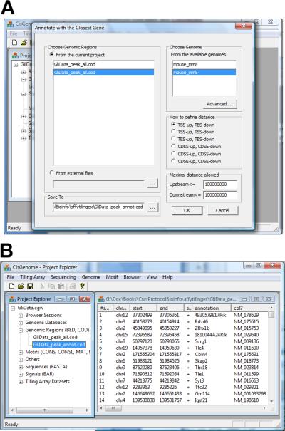
Peak-gene association. (A) The dialog for annotate peaks by nearby genes. (B) The annotation results returned in a COD file.
BASIC PROTOCOL 4
DNA SEQUENCE RETRIEVAL
This section introduces how to extract DNA sequences from a list of genomic regions. The extracted sequences can be used subsequently for motif discovery.
Necessary Resources
Hardware
A PC equipped with Windows OS.
Software
CisGenome (see Support Protocol 1).
Files
A list of genomic regions stored in a COD file (Figure 2.13.8)
A genome database for the species of interest (see Support Protocol 2)
Extract DNA Sequences
Load the genome database into CisGenome GUI (Support Protocol 2). For example, to extract DNA sequences from the peaks detected in the Gli example in Basic Protocol 1, load the mouse mm8 database.
Click the menu “Genome > Get Sequence”.
In the dialog that appears (Figure 2.13.16a), choose the peak list (COD file), choose the corresponding genome database, and specify a file (usually with *.fa suffix) to save the results.
(Optional) In the same dialog, choose a strand option. If the strand option is “Always + from assembly”, then the DNA sequences are extracted from the genome assembly as is. If the strand option is “Based on the coordinate file”, then for regions in the COD file annotated with “+” strand, the DNA sequences are extracted from the genome assembly as is; for regions annotated with “-” strand, DNA sequences will be extracted from the genome assembly, then the reverse complement of the extracted sequences will be returned.
- (Optional) In the same dialog, choose a conservation option. If “Get conservation scores” is not checked (default), only DNA sequences will be returned. Otherwise, both DNA sequences and phastCons cross-species conservation scores will be returned. The conservation scores can be returned in one of three formats:
- *.cs: a binary file with *.cs suffix will be created for each genomic region in the COD file. If a region is L base pairs long, then its corresponding CS file will contain L bytes. Each byte corresponds to a position in the region and is a number between 0 and 255. The number represents the conservation level, with 255 being the most conserved state. It is converted linearly from the phastCons conservation score at that position.
- .txt: a text file will be created for each genomic region (Figure 2.13.16b). Each line in the file corresponds to a position in the genomic region. The line contains a number between 0 and 255 to represent the conservation level.
- .bed: a BED file will be created for each genomic region (Figure 2.13.16b). Each line in the file corresponds to a position in the genomic region. The line contains chromosome, start coordinate, end coordinate, a space holder, and a number between 0 and 1000 to represent the conservation level (1000 represents the most conserved state).
Click “OK”. The program will start to run. When it is done, it will return DNA sequences in FASTA format (Figure 2.13.16b). If conservation score is requested in step 5, it will also return the conservation scores as described above.
Figure 2.13.16.
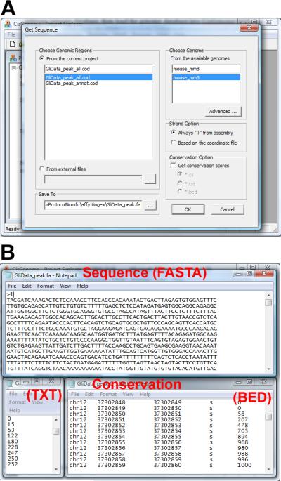
DNA sequence retrieval. (A) The parameter configuration dialog. (B) Returned files. The DNA sequences will be returned in FASTA format (top). If cross-species conservation score is requested, conservation scores for each sequence will be returned as well. The conservation scores can be returned in a text format (bottom left), in BED format (bottom right), or a binary CS format (not shown).
BASIC PROTOCOL 5
DE NOVO MOTIF DISCOVERY
This section introduces how to discover enriched DNA sequence motifs from protein-DNA binding regions without any prior knowledge about the motif patterns.
Necessary Resources
Hardware
A PC equipped with Windows OS.
Software
CisGenome (see Support Protocol 1).
File
A FASTA file that contains DNA sequences extracted from protein-DNA binding regions (see Basic Protocol 4). A sample sequence file Peak_ExonArray.fa can be downloaded from http://www.biostat.jhsph.edu/~hji/cisgenome/index_files/basicprotocol.htm. This file contains sequences from a collection of binding regions detected in the Gli data which are located near genes transcriptionally activated or repressed when Gli changes its expression.
Discover Novel DNA Motifs
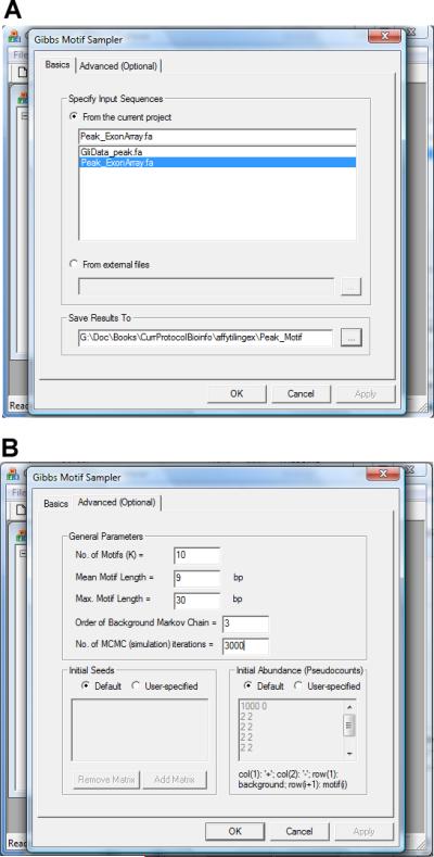
Load the FASTA sequence file into CisGenome using the menu “File > Load Data > Sequence”.
Click the menu “Motif > New Motif Discovery > Gibbs Motif Sampler”.
In the dialog that appears (Figure 2.13.17a), choose the FASTA file to be analyzed. Specify a folder and a file header to store the results.
- In the “Advanced (Optional)” tab of the dialog (Figure 2.13.17b), set the following parameters:
- No. of Motifs (K): number of motifs to be searched simultaneously.
- Mean Motif Length: the expected length (in base pairs) of a typical motif.
- Max. Motif Length: the maximal motif length allowed.
- Order of Background Markov Chain: DNA sequences not in the motif sites are modeled by a Markov Chain. This parameter specifies the order of the Markov Chain.
- No. of MCMC (simulation) iterations: CisGenome uses an iterative Gibbs sampling algorithm to search for motifs. This parameter specifies the number of iterations the algorithm will run.
- Initial Seeds and Initial Abundance: these are parameters used only by CisGenome developers. Check “Default”.
Click “OK”. The program will start to run. After it is done, it will generate a report file named [output file header]_motif_p.txt that summarizes the discovered motifs (Figure 2.13.18). See section on Guidelines for Understanding Results to learn more about this file.
Figure 2.13.17.
The parameter configuration dialog for de novo motif discovery.
Figure 2.13.18.
An example of the summary file produced by de novo motif discovery.
The motif matrix for each motif will also be saved to a file named [file header]_motif_[k].mat, following the MAT format (Figure 2.13.19a). A MAT file is a text file with four columns which correspond to A, C, G and T respectively. In the file, each line corresponds to a position within the motif, and each line contains four pseudo-numbers representing relative abundance of A, C, G and T. The MAT files can be used in subsequent motif mapping analysis.
The full paths of all MAT files are saved in a MATL file named [file header]_motif.matl. MATL stands for a list of MAT files. This is also a text file (Figure 2.13.19b).
The MAT and MATL files created by de novo motif discovery will be automatically added to the “Motifs” section in Project Explorer (Figure 2.13.19c). Double-clicking the MATL file will open a CisGenome browser window that shows the sequence logos (Crooks et al., 2004) of all discovered motifs.
Figure 2.13.19.
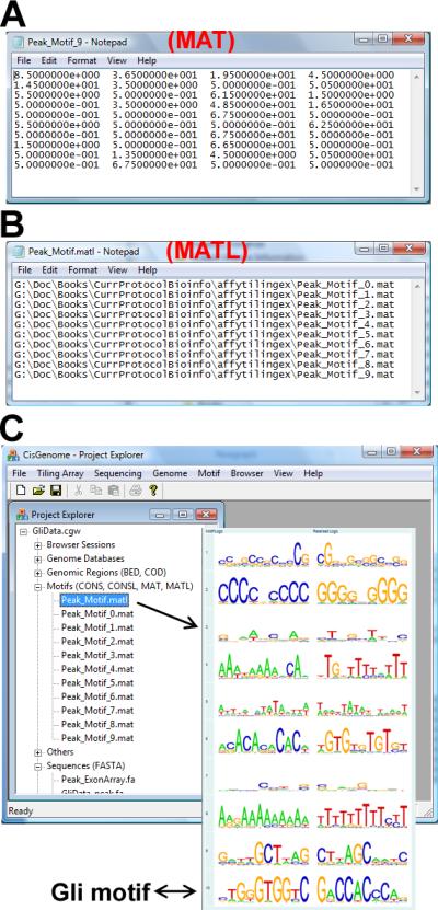
Motif matrix files produced by e novo motif discovery. (A) Each motif matrix is stored in a MAT file. (B) The list of motifs is stored in a MATL file. (C) Double-clicking the MATL file in Project Explorer opens CisGenome Browser to display sequence logos of the motifs. The last motif in this example matches the known Gli motif.
BASIC PROTOCOL 6
MOTIF MAPPING
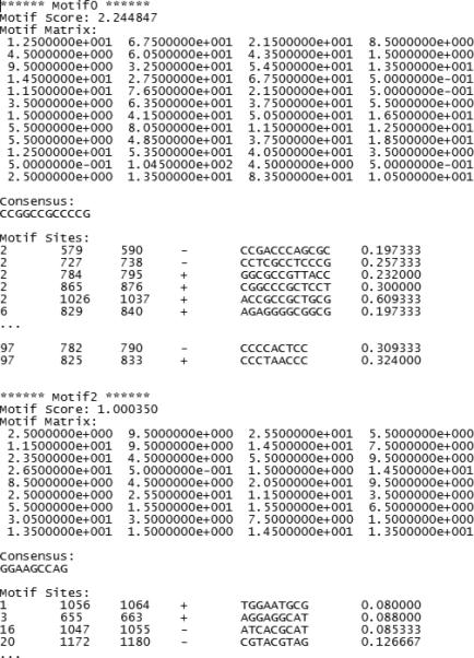
This section introduces how to map a motif to a list of genomic regions. CisGenome recognizes two ways to represent a motif, namely, motif matrix and consensus sequence. A motif matrix describes the relative abundance of A, C, G and T for each position of a motif. In CisGenome, it is stored in a MAT file (Figure 2.13.19a, also see Basic Protocol 5, step 5). To map a motif matrix to genome, CisGenome first converts the matrix into a probability matrix. It then scans the genome. At each genomic location, the likelihood of generating DNA from the motif matrix is compared to the likelihood of generating the same sequence from a background Markov model. If the likelihood ratio (LR) is bigger than a user-specified cutoff, then a motif site will be called.
A consensus sequence describes a motif by the most frequent nucleotide(s) at each position. In CisGenome, a consensus sequence is stored in a CONS file with *.cons suffix. The CONS file can be understood using the example shown in Figure 2.13.20. This example is a consensus sequence for the Gli binding motif. In this motif, the most frequent nucleotide at each position is TGGGTGGTC, respectively. At position 5, T can be replaced by A. At the last position, C can be replaced by A, G or T. For this motif, TGGGTGGTC is called the consensus sequence. TGGGT[A]GGTC[A,G,T] is called the degenerate consensus. If a genomic sequence has the following pattern TGAGAGGTG, then it has three Mismatches to the Consensus sequence (MC=3) and one Mismatch to the Degenerate consensus (MD=1). To map a consensus motif to genomic sequence, users first specify the maximal MC and MD allowed. CisGenome will scan the user-specified genomic regions and compare DNA sequences at each location to the consensus. All genomic loci with the MC and MD below the cutoffs will be reported as motif sites.
Figure 2.13.20.
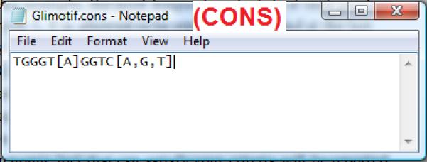
An example of the CONS file for describing motif consensus sequence.
Necessary Resources
Hardware
A PC equipped with Windows OS.
Software
CisGenome (see Support Protocol 1).
Files
A MAT or CONS file containing the motif. The matrix and consensus for Gli motif (Glimotif.mat, Glimotif.cons) will be used as examples. They can be downloaded from http://www.biostat.jhsph.edu/~hji/cisgenome/index_files/basicprotocol.htm
A COD file containing genomic regions to be analyzed (Figure 2.13.8)
A genome database for the species of interest (Support Protocol 2)
Map a Motif Matrix to a List of Genomic Regions
The procedure described below maps a motif to a COD file. By using the menu “Motif > Known Motif Mapping > Single Matrix –> FASTA” and following a similar procedure, one can also map a motif matrix to a FASTA sequence file.
Load the genome database into CisGenome GUI (see Support Protocol 2). For example, to map the Gli motif to the Gli binding regions identified in Basic Protocol 1, load the mouse mm8 database.
Load the motif matrix (e.g. Glimotif.mat) into CisGenome using the menu “File > Load Data > Motif > Matrix MAT”.
Load the list of genomic regions (COD file) to be analyzed into CisGenome using the menu “File > Load Data > Genomic Region”. For example, load GliData_peak_all.cod obtained in the Gli data analysis in Basic Protocol 1.
Click the menu “Motif > Known Motif Mapping > Single Matrix -> COD”.
- In the dialog that appears (Figure 2.13.21a), set parameters as follows:
- Choose the motif (i.e. MAT file) to be mapped.
- Choose the genome of interest.
- Choose the COD file that contains genomic regions to be analyzed.
- Specify an output file to store the results.
- Specify a likelihood ratio (LR) cutoff. By default, the cutoff is 500. Increasing the cutoff will increase stringency of the motif call.
- Choose a background type. One can either use the pre-computed Markov background models in the genome database, or estimate a background model from the input genomic regions.
- (Optional) Specify a criterion to filter motif sites by cross-species conservation. For example, keep sites that are located within the top 10% most conserved genome regions, or keep sites with conservation score no less than 40. In CisGenome, the conservation scores take values from 0 to 255, with 255 being the most conserved.
Click “OK” to start the analysis. After the analysis is done, all detected motif sites will be reported in a COD file and displayed in a window (Figure 2.13.21b).
Figure 2.13.21.
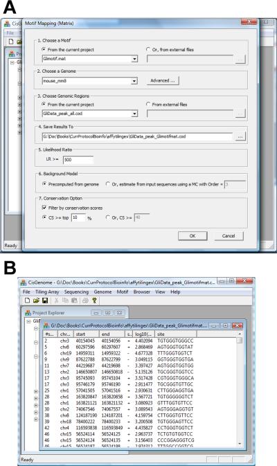
Mapping a motif matrix to a list of genomic regions. (A) The parameter configuration dialog. (B) The mapped motif sites are saved to a COD file.
Map a Motif Consensus Sequence to a List of Genomic Regions
The procedure is similar to mapping a motif matrix to a COD file. The differences are listed below. To map a motif consensus to a FASTA sequence file, use the menu “Motif > Known Motif Mapping > Single Consensus –> FASTA” and follow a similar procedure.
In step 2, use “File > Load Data > Motif > Consensus CONS” to load the consensus motif.
In step 4, click the menu “Motif > Known Motif Mapping > Single Consensus –> COD”.
In step 5e, instead of likelihood ratio, specify the maximal number of mismatches (MC) and the maximal number of degenerate mismatches (MD) allowed.
BASIC PROTOCOL 7
CHIP-CHIP PEAK CALLING FOR OTHER TILING ARRAY PLATFORMS
CisGenome can process ChIP-chip data generated by tiling array platforms other than Affymetrix arrays. This section introduces how to call peaks from these data.
Necessary Resources
Hardware
A PC equipped with Windows OS
Software
CisGenome (see Support Protocol 1)
Files
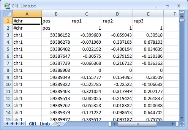
A tab-delimited text file containing the data (Figure 2.13.22). The first two columns of the file are chromosomes and coordinates of probes. For two color arrays, the remaining columns are log2 ratios between the ChIP and control channels. For one color arrays, the remaining columns are probe intensities. The first two rows of the file must start with “#chr”. The first row provides sample names, and the second row provides samples’ Group IDs (see Basic Protocol 1 steps 4b and 10c for meanings of Group IDs).
Figure 2.13.22.
Input data format for calling peaks from ChIP-chip experiments based on non-Affymetrix tiling array platforms.
A sample data set Gli1_Limb.txt can be downloaded from http://www.biostat.jhsph.edu/~hji/cisgenome/index_files/basicprotocol.htm. This is a ChIP-chip experiment for transcription factor Gli1 performed using Agilent two-color custom tiling arrays. There are three samples in the experiment, representing three biological replicates. All samples are assigned the same Group ID (=1). The data file contains log2(ChIP/control ratio) for each probe in each sample.
Normalize the Data
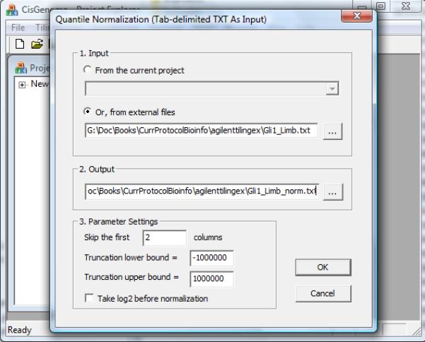
Click the menu “Tiling Array > Normalization > Quantile (TXT)”.
- In the dialog that appears (Figure 2.13.23), set parameters as follows:
- Choose the data file.
- Specify an output file to store the normalized data.
- Specify how many columns in the data file are not probe intensities. In the sample data Gli1_Limb.txt, the first two columns are genomic coordinates (Figure 2.13.22), therefore choose to skip the first two columns.
- Specify a truncation lower bound x and an upper bound y. Before normalization, any intensity value smaller than x will be truncated to x, and any intensity value bigger than y will be truncated to y.
- Specify whether the truncated data should be log2 transformed before normalization.
Click “OK”. The program will run and generate a new tab-delimited text file that contains normalized data. This file will be added to the Project Explorer under the “Others” section.
Figure 2.13.23.
The parameter configuration dialog for normalizing ChIP-chip data from a text file.
Convert the Normalized Data into a Tiling Array Data Set Consisting of BAR Files
-
4.
Click the menu “File > Load Data > Tiling Array Dataset > Import from TXT”.
-
5.In the dialog that appears (Figure 2.13.24a), set parameters as follows:
- Choose the text file that contains the normalized data.
- Specify an output file named with a *.cgw suffix to store the converted tiling array data set.
- If the probes are not sorted based on their genomic coordinates in the input file, check “Sort input”.
-
6.
Click “OK”. The normalized data will be converted into a new tiling array data set consisting of a number of BAR files (Figure 2.13.24b). Each BAR file contains the normalized intensities of a sample. These BAR files can be used for visualization (Basic Protocol 2).
Figure 2.13.24.
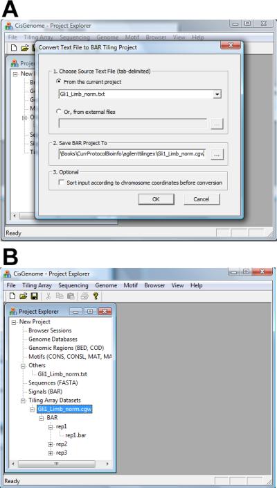
Converting ChIP-chip data in a text file to a tiling array data set consisting of BAR files. (A) The parameter configuration dialog. (B) The converted data set shown in Project Explorer.
Call Peaks and Perform Downstream Analysis
-
7.
Now follow Basic Protocol 1 steps 9-12 to perform peak calling. For the sample data Gli1_Limb.txt there is only one group, therefore set the peak calling type to be “One Sample Comparison” and set the pattern of interest to be “1>0.0”. This pattern will tell the program to look for genomic regions where the mean log2 (ChIP/control ratio) is bigger than zero. For data from one-color arrays, choose “Two Sample Comparison” or “Multiple Sample Comparison” in the same way as analyzing Affymetrix data. In all cases, the peak calling will produce the same files as the output of Basic Protocol 1.
-
8.
Follow Basic Protocols 2-6 to perform visualization and downstream analyses.
BASIC PROTOCOL 8
CHIP-SEQ PEAK CALLING (ONE-SAMPLE ANALYSIS)
In a ChIP-seq experiment, DNA fragments from chromatin immunoprecipitation samples are sequenced from both ends. The reads from sequencing are mapped to a reference genome. Protein-DNA binding regions are identified as regions with unexpected large number of reads. Depending on whether control samples are also sequenced, ChIP-seq experiments fall into two types. In a one-sample experiment, one only sequences ChIP samples. In a two-sample experiment, one sequences both ChIP and control samples. This section introduces how to call peaks from the one-sample experiment. After the peak calling, all subsequent analyses are the same as analyzing ChIP-chip data (see Basic Protocols 2-6).
Necessary Resources
Hardware
A PC with Windows OS and at least 4GB RAM
Software
CisGenome (see Support Protocol 1)
Files
A genome database for the species of interest (see Support Protocol 2)
A data file in the ALN format (Figure 2.13.25). The file contains alignments of sequence reads to the reference genome. An ALN file is a tab-delimited text file with three columns which are chromosome, position and strand (+/-, or F/R) respectively. A sample data (NRSF_ip_hg17.aln) from a ChIP-seq experiment for human transcriptional repressor NRSF can be downloaded from http://www.biostat.jhsph.edu/~hji/cisgenome/index_files/basicprotocol.htm.
Figure 2.13.25.
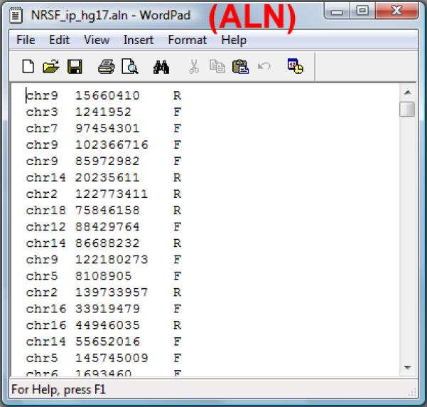
A sample ALN file.
Load Data
Load the genome database into CisGenome GUI (Support Protocol 2). For the sample data, use the human hg17 database.
Click the menu “Sequencing > Alignment –> BAR” to load the alignment (ALN) file (e.g. NRSF_ip_hg17.aln).
In the dialog that appears (Figure 2.13.26a), choose the data (ALN) file. If reads in the file have not been sorted by their coordinates, check “Sorting the input file(s) before conversion”. Otherwise leave the box unchecked.
Click “OK”. The ALN file will be converted into several BAR files which will be added to Project Explorer under the “Signals (BAR)” section (Figure 2.13.26b). The BAR file with the *_F.bar suffix contains locations of reads that are mapped to the “+” strand of the genome. The BAR file with the *_R.bar suffix contains locations of reads that are mapped to the “-” strand of the genome. The third BAR file contains locations of all reads.
Figure 2.13.26.
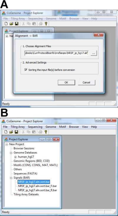
Loading aligned reads for ChIP-seq peak calling. (A) The parameter configuration dialog for loading the ALN file. (B) Loaded data shown in Project Explorer.
Compute FDR
Before peak detection, one has to choose a cutoff based on an estimate of the false discovery rate (FDR). This can be done as follows.
-
5.
Click the menu “Sequencing > One Sample Analysis > Exploration”.
-
6.
In the dialog that appears (Figure 2.13.27a), choose a genome, choose the BAR file obtained from step 4 that contains all reads, and specify an output file. Specify a window size W which is a positive integer. In the subsequent analysis, genome will be divided into non-overlapping W bp windows, and reads in each window will be counted.
-
7.
Click “OK”. The program will run and summarize data characteristics in a table (Figure 2.13.27b).
Figure 2.13.27.
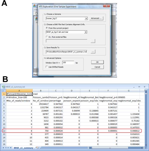
FDR computation for an one-sample ChIP-seq experiment. (A) The parameter configuration dialog. (B) The results are returned in a table that summarizes statistical properties of the data.
The table reports how many (column 2) and what fraction (column 3) of windows have exactly k reads (column 1). It also reports the expected proportion of windows that contain k reads under a Poisson background model (column 4), and the ratio between the expected proportion and the observed proportion under the Poisson model (column 5). In addition, the expected proportion of windows that contain k reads, and the ratio between the expected proportion and the observed proportion are also computed under a negative binomial background model (columns 6 and 7). The ratio in column 7 is usually used as an estimate of the FDR.
-
8.
Choose a cutoff for peak calling based on the estimated FDR in column 7. In the sample data, genomic windows with eight or more reads have an estimated FDR below 10%, thus the cutoff corresponding to FDR<10% is 8 reads per window.
Call Peaks
-
9.
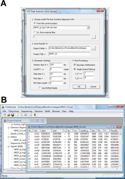
Click the menu “Sequencing > One Sample Analysis > Peak Detection”.
-
10.In the configuration dialog (Figure 2.13.28a), set parameters as follows:
- Choose the BAR file obtained in step 4 that contains all reads.
- Specify a folder to export the results.
- Specify a project title.
- Set the window size W, which should be equal to the window size used in FDR computation (i.e. step 6).
- Set a cutoff. This is the cutoff obtained from step 8. For the sample data, it is 8.
- Set a step size S. CisGenome will produce a read density BAR file for visualization. To generate this file, a W bp sliding window will be used to scan the genome at step size S.
- Set the “Max Gap” parameter. If two peaks are separated by less than Max_Gap bp, they will be merged into one peak.
- Set the “Min Peak Length”. Peaks shorter than this length will not be reported.
- (Optional) Check “Boundary Refinement”. If checked, CisGenome will analyze reads from the plus and minus strands separately. It then uses the modes of the two peaks on the plus strand and minus strand to define boundaries of a protein-DNA binding region.
- (Optional) Check “Single Strand Filtering”. If checked, also provide two cutoffs C_F and C_R. Peaks will not be reported if the number of plus strand reads < C_F and the number of minus strand reads < C_R for all W bp windows covered by the peak.
-
11.
Click “OK”. The program will run and produce a COD file that contains the detected peaks (Figure 2.13.28b).
Figure 2.13.28.
Peak calling from one-sample ChIP-seq data. (A) The parameter configuration dialog. (B) The detected peaks are reported in a COD file.
If you choose a peak and click the first column of the peak, you will be directed to CisGenome Browser which displays the peak signals. In addition, three BAR files named [project title].bar, [project title]_F.bar and [project title]_R.bar will be created and added to the Project Explorer. These files contain the total, plus strand, and minus strand window read count respectively.
BASIC PROTOCOL 9
CHIP-SEQ PEAK CALLING (TWO-SAMPLE ANALYSIS)
This section introduces how to use CisGenome to call peaks from a two-sample ChIP-seq experiment in which both ChIP and control samples are sequenced.
Necessary Resources
Hardware
A PC with Windows OS and at least 4GB RAM
Software
CisGenome (see Support Protocol 1)
Files
A genome database for the species of interest (see Support Protocol 2)
An ALN file (see Figure 2.13.25) that contains the alignments of ChIP reads to the reference genome
An ALN file that contains the alignments of control reads
A sample data set for NRSF with two files (ChIP: NRSF_ip_hg17.aln, control: NRSF_mock_hg17.aln) can be downloaded from http://www.biostat.jhsph.edu/~hji/cisgenome/index_files/basicprotocol.htm.
Load Data
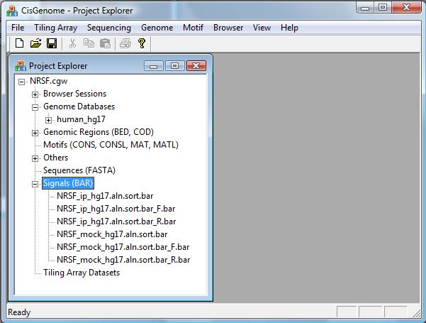
Follow Basic Protocol 8 steps 1-4 to load the genome database (hg17 for the sample data) and all alignment files into CisGenome (Figure 2.13.29).
Figure 2.13.29.
Data for two-sample ChIP-seq analysis loaded into CisGenome.
Compute FDR
-
2.
Click the menu “Sequencing > Two Sample Analysis > Exploration”.
-
3.In the configuration dialog that appears (Figure 2.13.30a), specify parameters as follows.
- Choose a genome database.
- Choose a positive BAR file that contains all reads in the ChIP sample.
- Choose a negative BAR file that contains all reads in the control sample.
- Specify an output file to store the results.
- Specify a window size W.
-
4.
Click “OK”. The program will run and return a summary of data characteristics (Figure 2.13.30b). This summary is very similar to the summary table produced by the one-sample analysis (see Basic Protocol 8, step 7). However, the summary here is computed after combining ChIP and control reads.
Figure 2.13.30.
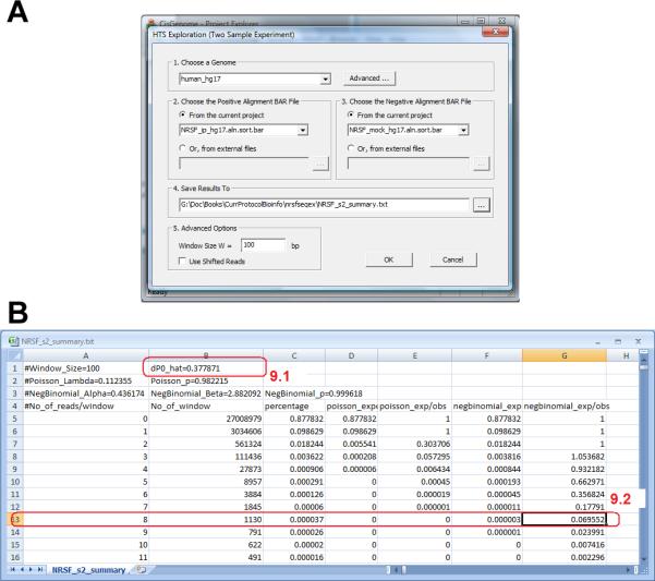
FDR computation for a two-sample ChIP-seq experiment. (A) The parameter configuration dialog. (B) The results are returned in a table that summarizes statistical properties of the data.
There is a new quantity called “dP0_hat” (Figure 2.13.30b, circle 9.1). This is an estimate of the expected proportion of ChIP reads in background genomic windows. In other words, let k1 be the number of ChIP reads in a window, k2 be the number of control reads in the same window, and n=k1+k2, then dP0_hat estimates E[k1/n | no protein-DNA binding]. This estimate is used to determine whether a (n, k1) pair represents a statistically significant enrichment.
The program also generates a file named “[outputfile].fdr” in the output folder. This file contains FDR computed for all (n, k1) pairs based on dP0_hat.
Call Peaks
-
5.
Click the menu “Sequencing > Two Sample Analysis > Peak Detection”.
-
6.In the configuration dialog (Figure 2.13.31), set parameters as follows:
- Choose the positive BAR file that contains all ChIP reads.
- Choose the negative BAR file that contains all control reads.
- Specify a working folder to store the results, and specify a project title.
- Specify a FDR file and an FDR cutoff. The FDR file is the file with the *.fdr suffix generated in step 4. It contains pre-computed FDR for all (n, k1) pairs. For the sample NRSF data, choose 0.1 (i.e. 10%) as the FDR cutoff.
- Provide the expected proportion of ChIP reads in background genomic regions. This is the dP0_hat obtained in step 4 (dP0_hat=0.377871 for the NRSF example).
- Set a window size W, which should be consistent with the window size used in FDR computation.
- Specify “Min Read Num M”. This is the minimal total read count n a window must have in order to be considered for peak calling. Windows with read count smaller than this number will be excluded from peak detection. Usually, this number is obtained by examining the summary file in step 4. For the NRSF example, windows with 8 or more reads have a one-sample FDR <10% based on the negative binomial model (Figure 2.13.30b, circle 9.2). Therefore we choose 8 as the Min Read Num.
- Set step size S. CisGenome will produce several read density BAR files for visualization. To generate these files, a W bp sliding window with step size S will be used to scan the genome.
- Set Max Gap (see Basic Protocol 8, step 10g).
- Set Min Peak Length (see Basic Protocol 8, step 10h).
- (Optional) If you want to find regions where the ChIP read count is more than expected as well as regions where the ChIP read count is less than expected given the control read count, check “Two-sided Test”. If you only want to find regions where the ChIP read count is more than expected, leave the box unchecked (default).
- (Optional) Check “Boundary Refinement” (see Basic Protocol 8, step 10i).
- (Optional) Check “Single Strand Filtering” and provide C_F and C_R (see Basic Protocol 8, step 10j).
-
12.
Click “OK”. The program will run and report peaks in a COD file. If you choose a peak and click the first column of the peak, you will be directed to CisGenome Browser which displays the peak signals. In addition, a number of BAR files will be created for visualization.
Figure 2.13.31.
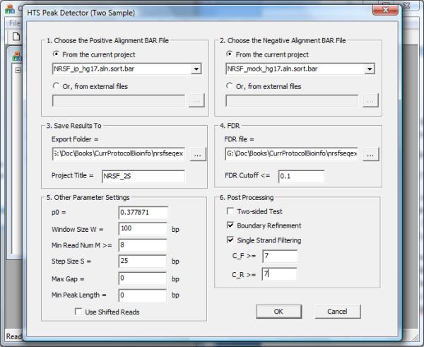
The parameter configuration dialog for two-sample ChIP-seq peak calling.
SUPPORT PROTOCOL 1
INSTALLING CISGENOME
Necessary Resources
Hardware
A PC equipped with Windows OS
Software
WinZip or WinRAR, a text editor such as Notepad or Wordpad
Install CisGenome
Download CisGenome Windows (GUI, Browser and Core Programs) from http://www.biostat.jhsph.edu/~hji/cisgenome/index_files/download.htm.
Save the downloaded file to a folder that does not contain any blank characters such as spaces or tabs. For example, one can save it to D:\Projects\cisgenome_project\.
Unzip the downloaded file using WinZip or WinRAR.
In the uncompressed folder, locate a file named “CisGenome.exe” and another file called “CisGenome.ini”.
Open CisGenome.ini using a text editor (e.g. Notepad). Edit the file to provide CisGenome installation folder in the following format “CisGenome=[installation folder]”. Do not add any blank characters such as spaces before and after “=”. A sample CisGenome.ini file is shown in Figure 2.13.32.
Save CisGenome.ini and close it.
Double-click CisGenome.exe. CisGenome will start. You will see its graphic user interface (GUI).
Figure 2.13.32.
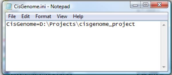
An example of the CisGenome.ini file.
SUPPORT PROTOCOL 2
INSTALLING GENOME DATABASES
A number of CisGenome analysis functions require information about the genome, including genomic DNA sequences, cross-species conservation, and gene annotations. The information is usually stored in pre-complied genome databases which can be downloaded from CisGenome website. This unit introduces how to install a genome database.
Necessary Resources
Hardware
A PC equipped with Windows OS
Software
WinZip or WinRAR
CisGenome (see Support Protocol 1)
Install a Genome Database
Download the genome database for the species of interest from the following webpage http://www.biostat.jhsph.edu/~hji/cisgenome/index_files/download.htm.
Unzip the downloaded database using WinZip or WinRAR.
Check the unzipped folder. It should contain several subfolders and a number of files. One of the files should be named as [species]_[assembly].cgw (e.g. mouse_mm8.cgw).
Load the Installed Genome Database into CisGenome
-
4.
Click the menu “File > Load Data > Genome Database”.
-
5.
A dialog will appear (Figure 2.13.33a). In the dialog, enter the folder in which the genome database is installed.
-
6.
Find the file named [species]_[assembly].cgw (e.g. mouse_mm8.cgw). Click on the file to select it, then click “Open”.
-
7.
Check whether the database is successfully loaded. If successful, one should see the database in the “Project Explorer” window. The name of the database will appear under the section titled “Genome Databases” (Figure 2.13.33b).
Figure 2.13.33.

Load a genome database into CisGenome GUI. (A) In the file open dialog, choose the file named [species]_[assembly].cgw in the genome database folder. (B) The loaded database shown in Project Explorer.
GUIDELINES FOR UNDERSTANDING RESULTS
Results from ChIP-chip Peak Calling (Basic Protocols 1 and 7)
CisGenome uses the TileMap algorithm (Ji and Wong, 1995) to call peaks from ChIP-chip data. The program will create the following files in the output folder (Figure 2.13.8).
A BAR file with a *.fc.bar suffix. This file is a binary file that stores log2 (ChIP/control fold change) for all probes. If the ChIP-chip data set contains multiple array platforms (e.g. the Affymetrix Mouse Tiling 2.0R array set contains seven arrays with seven different BPMAP files), then a BAR file is generated for each array platform. The BAR files can be used for visualizing enrichment signals in the CisGenome Browser (Basic Protocol 2).
A BAR file with *.ma.bar (if the TileMap Moving Average (MA) method was used to call peaks) or *.hmm.bar suffix (if the TileMap Hidden Markov Model (HMM) approach was used for peak calling) for each array platform. These files store the TileMap MA statistics or HMM posterior probabilities for protein-DNA binding. They can also be used for visualization.
A COD file with a *.cod suffix. This file contains the list of detected peaks (Figure 2.13.8). The columns of the file are explained in Table 2.13.2. Column 9 of this file provides a FDR estimate for each peak. Users should look at the FDR and construct a final peak list using a FDR cutoff they are comfortable with (usually FDR = 10% or less). Usually, we recommend removing peaks below the FDR cutoff from the COD file before one proceeds to the subsequent analyses. Sometimes, the COD file may contain a number of peaks, but none of them have an acceptable FDR (e.g. all FDR > 50%). This is an indication of noisy data, and no peak can be confidently called. One should examine the enrichment signals visually to understand why.
Table 2.13.2.
Columns of the COD file produced by ChIP-chip peak calling
| Column | Description |
|---|---|
| 1 | Peak rank |
| 2 | Chromosome |
| 3 | Peak start |
| 4 | Peak end |
| 5 | Peak strand (+ for all peaks) |
| 6 | Peak length |
| 7 | maxM/P: the maximal TileMap-MA statistic or maximal HMM posterior probability of all probes within the peak. |
| 8 | Genomic coordinate of the probe where the maxM/P is achieved |
| 9 | FDR: false discovery rate based on MaxM/P. |
| 10 | local_FDR: local false discovery rate based on MaxM/P. |
| 11 | maxFC(log2): the maximal log2(ChIP/control fold change) within the peak. |
| 12 | Genomic coordinate of the probe where the maxFC is achieved |
| 13 | sumM/P: the sum of MA statistics or HMM probabilities of all good probes within the peak. Good probes are probes not filtered out because they are masked or labeled as outliers in CEL files. |
| 14 | Number of good probes used to compute sumM/P. |
| 15 | sumM/P_FDR: false discovery rate based on sumM/P. |
| 16 | sumM/P_local_FDR: local false discovery rate based on sumM/P. |
| 17 | library_id: an identifier for array platform. For example, if one uses Mouse Tiling 2.0R 7 array set, then the seven arrays are labeled as 1, 2, ..., 7. |
| 18 | group_name: name of the genome assembly used in the BPMAP file for probe coordinates. |
Results from Peak-Gene Association (Basic Protocol 3)
CisGenome will return a COD file in the output folder (Figure 2.13.15b). The file contains information of the gene closest to each peak in the input COD file. Columns in the output file are peak identifier, chromosome, peak start, peak end, peak strand, name of the closest gene, RefSeq ID of the closest gene, gene's chromosome, gene's strand, gene's TSS, TES, CDSS, CDSE, gene's exon number, start coordinates of exons (separated by comma), and end coordinates of exons (separated by comma).
Results from De Novo Motif Discovery (Basic Protocol 5)
CisGenome will produce three types of files, all starting with the user-specified output file header.
[file header]_motif_[k].mat: these are files that contain the motif matrices in MAT format (Figure 2.13.19a). If the program is asked to search for K motifs, then there will be K such files, one for each motif. Here [k] is an integer from 0 to K-1.
[file header]_motif.matl: this is a text file in MATL format that contains full paths of all MAT files produced by the motif discovery (Figure 2.13.19b).
[file header]_motif_p.txt: this is a text file that summarizes information for all identified motifs and motif sites (Figure 2.13.18). The file has K sections, one for each motif. Each section starts with a motif score to describe the strength of the motif. A motif with good quality usually has a score bigger than 1.5. The motif matrix and consensus sequence are then provided. Subsequently, all identified motif sites are also given. Each site is described by its origin sequence id (e.g. 0 = the first sequence in the input FASTA file, 1= the second sequence, etc.), its start and end coordinates in the origin sequence, its strand in the origin sequence, the DNA sequence of the site, and a score to characterize how well the site matches the motif matrix (the bigger the score the better).
Results from Motif Mapping (Basic Protocol 6)
The result of mapping a motif matrix to a list genomic regions (in a COD file) or sequences (in a FASTA file) is a COD file that reports all detected motif sites (Figure 2.13.21b). The columns of the file are identifier of the genomic region or sequence in which the site is found, chromosome (if the input file is COD) or sequence id (if the input is FASTA) of the motif site, motif site start coordinate, site end, site strand, log10 likelihood ratio between the motif model and background model at the site, and DNA sequences in the site.
The result of mapping a motif consensus sequence to genome is similar. The only difference is that the log10 likelihood ratio column in the output COD file is replaced by a negative score –X.Y, where X is the number of degenerate mismatches (MD), and Y is the number of mismatches (MC) of the site compared to the consensus.
Results from One-sample ChIP-seq Peak Calling (Basic Protocol 8)
CisGenome peak calling from one-sample ChIP-seq experiment will produce the following files in the output folder.
Three BAR files named as [project title].bar, [project title]_F.bar and [project title]_R.bar. These files contain the total, plus strand, and minus strand window read count for the genome. They can be used for visualizing enrichment signals in CisGenome Browser.
A COD file that contains all peaks detected at the user-specified FDR cutoff. The fields in this COD file are listed in Table 2.13.3. One can open the file using EXCEL and further filter peaks based on, for instance, the number of reads in the peak or peak length.
Table 2.13.3.
Columns of the COD file produced by one-sample ChIP-seq peak calling
| Column | Description |
|---|---|
| 1 | Peak rank |
| 2 | Chromosome |
| 3 | Peak start |
| 4 | Peak end |
| 5 | Peak strand (+ for all peaks) |
| 6 | Peak length |
| 7 | maxN: the maximal read count of all W bp windows covered by the peak. W is the window width used for peak detection. |
| 8 | maxN_pos: genomic coordinate of the center of the W bp window where the maxN is achieved. |
| 9 | total_reads: total read count in the peak. |
| 10 | Ftot_reads: total count of reads on the plus strand. |
| 11 | FmaxN: the maximal + strand read count for all W bp windows within the peak. |
| 12 | FmaxN_pos: the center position of the W bp window where the FmaxN is achieved. |
| 13 | Rtot_reads: total count of reads on the minus strand. |
| 14 | RmaxN: the maximal - strand read count for all W bp windows within the peak. |
| 15 | RmaxN_pos: the center position of the W bp window where the RmaxN is achieved. |
| 16 | Rmaxpos-Fmaxpos: distance between the plus strand peak and the minus strand peak, i.e. RmaxN_pos -FmaxN_pos+1 |
| 17 | Delta = [min(FmaxN, RmaxN)+1]/[max(FmaxN, RmaxN)+1] |
Results from Two-sample ChIP-seq Peak Calling (Basic Protocol 9)
CisGenome peak calling from two-sample ChIP-seq experiment will produce the following files in the output folder.
-
(1)Seven BAR files listed below.
- *.pos.bar: ChIP read counts in a W bp window sliding across the genome at step size S.
- *.neg.bar: Control read counts in a W bp window sliding at step size S.
- *_F.pos.bar and *_F.neg.bar: Plus strand window read counts for ChIP and control samples.
- *_R.pos.bar and *_R.neg.bar: Minus strand window read counts for ChIP and control samples.
- *.log2fc.bar: log2[(ChIP read count + 1)/(Control read count +1)] for a W bp window sliding across the genome at step size S.
These BAR files can be used for visualizing enrichment signals in CisGenome Browser.
-
(2)
A COD file that contains all peaks detected at the user-specified FDR level. The fields in this COD file are listed in Table 2.13.4. One can open the file using EXCEL and further filter peaks based on, for instance, max|FC| or number of reads in the peak.
Table 2.13.4.
Columns of the COD file produced by two-sample ChIP-seq peak calling
| Column | Description |
|---|---|
| 1 | Peak rank |
| 2 | Chromosome |
| 3 | Peak start |
| 4 | Peak end |
| 5 | Peak strand (+ for all peaks) |
| 6 | Peak length |
| 7 | minFDR: the minimal false discovery rate for all W bp windows within the peak. |
| 8 | minFDR_pos: the center coordinate of the W bp window in which the minFDR is achieved |
| 9 | max|FC|: the maximal |log2(ChIP/control read count fold change)| for all W bp windows within the peak |
| 10 | max|FC|_pos: the center coordinate of the W bp window in which the max|FC| is achieved |
| 11 | pos_read_num: number of ChIP reads within the peak |
| 12 | neg_read_num: number of control reads within the peak |
| 13-18 | Information for plus strand reads. These are counterparts to columns 7-12. |
| 19 | Fmaxpos_readnum: the maximal number of plus strand ChIP reads for all W bp windows within the peak |
| 20 | Fmaxpos_readnum_pos: the center of the W bp window in which the Fmaxpos_readnum is achieved |
| 21 | Fmaxneg_readnum: the maximal number of plus strand control reads for all W bp windows within the peak |
| 22 | Fmaxneg_readnum_pos: the center of the W bp window in which the Fmaxneg_readnum is achieved |
| 23-32 | Information for minus strand reads. These are counterparts to columns 13-22. |
| 33 | Rmode-Fmode: distance between the plus strand peak and the minus strand peak |
| 34 | Delta = {2^min(5' max|FC|, 3' max|FC|)}/2^(max(5' max|FC|, 3' max|FC|)} |
| 35 | maxPosN: the maximal number of ChIP reads for all W bp windows within the peak. |
| 36 | maxPosN_pos: the center of the W bp window in which the maxPosN is achieved |
| 37 | maxNegN: the maximal number of control reads for all W bp windows within the peak. |
| 38 | maxNegN_pos: the center of the W bp window in which the maxNegN is achieved. |
COMMENTARY
Background Information
ChIP-chip Peak Calling
CisGenome uses TileMap (Ji and Wong, 2005) to call peaks from ChIP-chip data. The TileMap algorithm first performs quantile normalization (Bolstad et al., 2003) of ChIP-chip samples. It then uses a two-step procedure to call peaks. In the first step, the enrichment signal at each probe is summarized by a t-statistic. The t-statistic compares probe intensities in ChIP samples with those in control samples. The variance of the t-statistic is modified via an empirical Bayes shrinkage estimator to improve performance in scenarios where the number of replicate samples is small. In the second step, information from neighboring probes is combined to infer peak status of a probe. This is done by using either a moving average (MA) method or a Hidden Markov Model (HMM). In the MA method, a moving window is used to scan the genome, and t-statistics within the window are averaged. If the average is bigger than a user-specified cutoff, then the window will be chosen to create a binding region. Selected windows that are overlapping will be merged. After merging, the set of non-overlapping binding regions will be reported. In the HMM method, each probe is assumed to be generated either from a background state or from a binding state. A forward-backward algorithm is used to decode the unknown state of each probe. Probes with posterior probability in the binding state bigger than a user-specified cutoff will be picked up to construct binding regions. By default, CisGenome uses the TileMap-MA to call peaks. However, users can choose to use HMM by going to the “Advanced Settings (Optional)” tab in Figure 2.13.7 and check the HMM option. Readers are referred to Ji and Wong (2005) to learn details about the TileMap algorithm.
ChIP-seq Peak Calling
For one-sample ChIP-seq peak calling, CisGenome uses a W bp sliding window to scan the genome. The number of reads in the window is counted. If the window does not contain a binding site, its read count approximately follows a negative binomial distribution. The parameters of this distribution can be estimated from the data. Using this negative binomial as the noise model, one can determine a read count cutoff c such that among all windows passing this cutoff (i.e. having ≥ c reads), only x percent are expected to be background noise. In other words, c controls the FDR to be x%. All windows above this cutoff will then be selected. Overlapping windows are merged. The non-overlapping regions resulted from this analysis create the predicted peak list. For “boundary refinement”, the same analysis will be performed separately for plus strand and negative strand reads. Peaks detected from the two strands typically are shifted by certain amount of base pairs due to the nature of the technology, as reads are obtained from two ends of DNA fragments and protein associates with DNA somewhere in the middle. One can use the peak on the plus strand and the peak on the minus strand to narrow down the binding site location. CisGenome takes advantage of this and uses the two modes from the plus and minus strand peaks to define the binding site boundaries. For “single strand filtering”, peaks with unbalanced plus and minus strand read counts are filtered away. For visualization, window read counts are saved to BAR files every S base pairs, where S is the step size.
For two-sample ChIP-seq peak calling, a sliding window is used to scan the genome. For each window, the number of ChIP and control reads are counted and denoted as k1 and k2 respectively. Let n = k1+ k2. It is assumed that if there is no binding, k1 | n follows a binomial distribution B(n, p0). p0 can be estimated from the data. Using the estimated p0 (i.e. dP0_hat), one can determine the FDR for each k1 under a fixed n. Users provide a FDR cutoff, all windows with FDR smaller than the cutoff will be used to create binding regions. Readers are referred to Ji et al. (2008) for details of the one-sample and two-sample ChIP-seq analysis algorithms.
De novo Motif Discovery
CisGenome uses the Gibbs motif sampler described in Liu et al. (1995) to perform de novo motif discovery. Briefly, DNA sequences are described by a generative probabilistic model. Each position in the sequences is assumed to be generated either from a background Markov model or from one of K possible motif models. Each motif model is described by a matrix in which each column is a probability vector describing probabilities to generate A, C, G and T. The Gibbs motif sampler iteratively estimates locations of motif sites given the current estimate of the motif matrices, and re-estimates the motif matrices given the current locations of motif sites. After a number of iterations, the Gibbs sampler will converge and the motif patterns will emerge. A score is assigned to each motif to characterize its strength. The score is the log(n) * [the average information content per nucleotide], where n is the number of detected sites for the motif. This is essentially the MDSCAN motif score under a zeroth-order Markov background model (Liu et al., 2002). Readers are referred to Liu et al. (1995) and Jensen et al. (2004) for details of the model and algorithm, and to Liu et al. (2002) for description of the motif score.
Motif Mapping
CisGenome can map both consensus sequences and motif matrices to user-specified genomic regions. In order to map a consensus sequence, the consensus is used to scan the genome. At each position of the genome, the number of mismatch (MC) bases and degenerate mismatches (MD) are counted as described in Basic Protocol 6. A position is called a motif site if its MC and MD do not exceed the user-specified cutoffs.
In order to map a motif matrix, the matrix is used to scan the genome. At each position, the likelihood ratio (LR) between the motif model and a third order background Markov model is computed. Sites with LR bigger than the user-chosen cutoff will be reported.
Critical Parameters and Troubleshooting
Installation
(1) “I can start CisGenome by clicking CisGenome.exe, but none of my CisGenome functions seem to work. Why?”
First, check whether CisGenome is installed in a folder that does not contain any blank characters such as spaces or tabs in the folder name. It is important to keep in mind that if CisGenome is installed in folders with blank characters, it will not function properly. For example, the folder “C:\Document and Settings\CisGenome” cannot serve as an installation folder. An example of a valid folder is “D:\Projects\cisgenome_project”.
Second, check whether you have configured the file named “CisGenome.ini” (Figure 2.13.32). In this file, one has to provide the CisGenome installation folder (Support Protocol 1). Otherwise, the GUI does not know where to find executable programs to carry out the analyses.
Third, check the names of folders and files used in the analysis. None of the folder or file names should contain any blank characters. If they do, CisGenome may not run properly.
(2) “There are multiple genome databases for each species. Which one should I use?”
Download and install the database that is consistent with your ChIP-chip or ChIP-seq data. For example, if the ChIP-chip data are from mouse and probes in the tiling array are mapped to the mm8 genome assembly, then download the mouse mm8 database (instead of mm7 or mm9). If you have human ChIP-seq data and reads are aligned to hg19 genome assembly, then download human hg19 database. It is important that the genome assembly used for peak calling must be consistent with the genome database used in the downstream analyses.
ChIP-chip peak calling
(3) “How can I choose the window size parameter for TileMap-MA?”
It depends on the DNA fragment length x and the average distance between two neighboring probes y. It is estimated that a typical peak should contain x/y probes, therefore the half window size is x/(2y) probes and x/2 base pairs.
(4) “I have obtained a list of peaks, but none of them have FDR < 5%. How should I interpret the results?”
FDR below 25% is usually acceptable. However, if none of your peak has FDR < 50%, then your data might be too noisy. Visually examine the enrichment signals (Basic Protocols 1 and 2) to figure out what is going on.
ChIP-seq peak calling
(5) “What window size should I use for ChIP-seq peak calling?”
Usually we use 100-200 bps for transcription factors. For chromatin marks, the window size should approximately be the same as the average length of the mark signal. One can visually examine the data in the CisGenome Browser to estimate this length.
(6) “When I use CisGenome to perform one-sample analysis, the summary file obtained from FDR computation shows NaN in the columns ‘negbinomial_expected’ and ‘negbinomial_exp/obs’. How should I interpret the result and choose a cutoff?”
NaNs are commonly caused by two reasons. First, multiple reads can align to exactly the same genomic position. Frequently these are due to technical biases. These biases can make the distribution of window read count dramatically different from a negative binomial model, resulting in bad model fitting. To avoid such biases, it is recommended to keep only one read at each unique genomic position. The problem will often go away if the user-supplied ALN file contains only these non-redundant reads. Second, artifacts we are unaware of can be another major reason. Therefore, if the problem still exists after you removed redundant reads, visually examine the BAR files converted from the ALN files in the CisGenome Browser and check whether the data have strong artifacts.
(7) “When I perform ChIP-seq peak calling, CisGenome starts to run but stops quickly without producing any output file. What was the problem?”
Most likely, the memory in your PC is not sufficient. Try to increase the step size parameter S in Figure 2.13.28a and 2.13.31. The reason is explained below. During the peak calling, CisGenome will create BAR files that contain enrichment signals. The BAR files will store a data point every S base pairs. When S is small, lots of memory is required to create these BAR files. This often causes insufficient memory. By setting S to a bigger number (e.g. 100 instead of the default 25), you will significantly reduce the memory requirement without affecting peak detection. The new S will only affect the resolution you can achieve in the visualization. Keep in mind that S is not allowed to be bigger than W.
Visualization
(8) “I used CisGenome to call peaks from my Affymetrix Tiling array data. I obtained the COD file and BAR files. However, when I was trying to visualize the BAR files, I cannot see any probe. What was wrong?”
Very likely you have used a BPMAP file provided by Affymetrix that has named chromosomes in a non-standard way (e.g. NCBIv33:chr6 instead of chr6). In these cases, using the BPMAP file downloaded from the CisGenome website to reanalyze the data should solve the problem.
De novo motif discovery
(9) “The de novo motif discovery takes a long time to run. How can I improve its efficiency?”
If you run motif discovery using all peaks reported from peak detection, it will be computationally intensive. For example, searching 20 motifs simultaneously in 1000 peaks, each 1000 bp long, and running 5000 iterations of Gibbs Sampler could take 12-48 hours depending on your computer. Usually, to discover new motifs, it is not necessary to use all peaks. You can use a small number of top peaks (e.g. top 200 peaks) and search for a smaller number of motifs (e.g. 10), which will reduce the computation time. The computation time is linear to the number of motifs you are searching for, total length of input DNA sequences, and the number of iterations you run.
Acknowledgement
The work is partially supported by National Institutes of Health grants R01HG004634 (Wing Hung Wong) and R01HG005220 (Hongkai Ji).
Literature Cited
- Barski A, Cuddapah S, Cui K, Roh TY, Schones DE, Wang Z, Wei G, Chepelev I, Zhao K. High-resolution profiling of histone methylations in the human genome. Cell. 2007;129:823–837. doi: 10.1016/j.cell.2007.05.009. [DOI] [PubMed] [Google Scholar]
- Bolstad BM, Irizarry RA, Astrand M, Speed TP. A comparison of normalization methods for high density oligonucleotide array data based on variance and bias. Bioinformatics. 2003;19:185–193. doi: 10.1093/bioinformatics/19.2.185. [DOI] [PubMed] [Google Scholar]
- Cawley S, Bekiranov S, Ng HH, Kapranov P, Sekinger EA, Kampa D, Piccolboni A, Sementchenko V, Cheng J, Williams AJ, Wheeler R, Wong B, Drenkow J, Yamanaka M, Patel S, Brubaker S, Tammana H, Helt G, Struhl K, Gingeras TR. Unbiased mapping of transcription factor binding sites along human chromosomes 21 and 22 points to widespread regulation of noncoding RNAs. Cell. 2004;116:499–509. doi: 10.1016/s0092-8674(04)00127-8. [DOI] [PubMed] [Google Scholar]
- Crooks GE, Hon G, Chandonia JM, Brenner SE. WebLogo: A sequence logo generator. Genome Res. 2004;14:1188–1190. doi: 10.1101/gr.849004. [DOI] [PMC free article] [PubMed] [Google Scholar]
- Jensen ST, Liu XS, Zhou Q, Liu JS. Computational discovery of gene regulatory binding motifs: a Bayesian perspective. Statistical Science. 2004;19:188–204. [Google Scholar]
- Ji H, Wong WH. TileMap: create chromosomal map of tiling array hybridizations. Bioinformatics. 2005;21:3629–3636. doi: 10.1093/bioinformatics/bti593. [DOI] [PubMed] [Google Scholar]
- Ji H, Jiang H, Ma W, Johnson DS, Myers RM, Wong WH. An integrated software system for analyzing ChIP-chip and ChIP-seq data. Nat Biotechnol. 2008;26:1293–1300. doi: 10.1038/nbt.1505. [DOI] [PMC free article] [PubMed] [Google Scholar]
- Johnson DS, Mortazavi A, Myers RM, Wold B. Genome-wide mapping of in vivo protein-DNA interactions. Science. 2007;316:1497–1502. doi: 10.1126/science.1141319. [DOI] [PubMed] [Google Scholar]
- Liu JS, Neuwald AF, Lawrence CE. Bayesian models for multiple local sequence alignment and Gibbs sampling strategies. J. Amer. Statist. Assoc. 1995;90:1156–1170. [Google Scholar]
- Liu XS, Brutlag DL, Liu JS. An algorithm for finding protein-DNA binding sites with applications to chromatin-immunoprecipitation microarray experiments. Nat. Biotechnol. 2002;20:835–839. doi: 10.1038/nbt717. [DOI] [PubMed] [Google Scholar]
- Mikkelsen TS, Ku M, Jaffe DB, Issac B, Lieberman E, Giannoukos G, Alvarez P, Brockman W, Kim TK, Koche RP, Lee W, Mendenhall E, O'Donovan A, Presser A, Russ C, Xie X, Meissner A, Wernig M, Jaenisch R, Nusbaum C, Lander ES, Bernstein BE. Genome-wide maps of chromatin state in pluripotent and lineage-committed cells. Nature. 2007;448:553–560. doi: 10.1038/nature06008. [DOI] [PMC free article] [PubMed] [Google Scholar]
- Ren B, Robert F, Wyrick JJ, Aparicio O, Jennings EG, Simon I, Zeitlinger J, Schreiber J, Hannett N, Kanin E, Volkert TL, Wilson CJ, Bell SP, Young RA. Genome-wide location and function of DNA binding proteins. Science. 2000;290:2306–2309. doi: 10.1126/science.290.5500.2306. [DOI] [PubMed] [Google Scholar]
- Robertson G, Hirst M, Bainbridge M, Bilenky M, Zhao Y, Zeng T, Euskirchen G, Bernier B, Varhol R, Delaney A, Thiessen N, Griffith OL, He A, Marra M, Snyder M, Jones S. Genome-wide profiles of STAT1 DNA association using chromatin immunoprecipitation and massively parallel sequencing. Nat Methods. 2007;4:651–657. doi: 10.1038/nmeth1068. [DOI] [PubMed] [Google Scholar]
- The Gene Ontology Consortium Gene ontology: tool for the unification of biology. Nat Genet. 2000;25:25–29. doi: 10.1038/75556. [DOI] [PMC free article] [PubMed] [Google Scholar]
- Siepel A, Bejerano G, Pedersen JS, Hinrichs AS, Hou M, Rosenbloom K, Clawson H, Spieth J, Hillier LW, Richards S, Weinstock GM, Wilson RK, Gibbs RA, Kent WJ, Miller W, Haussler D. Evolutionarily conserved elements in vertebrate, insect, worm, and yeast genomes. Genome Res. 2005;15:1034–1050. doi: 10.1101/gr.3715005. [DOI] [PMC free article] [PubMed] [Google Scholar]